This document contains summaries of key concepts in engineering economics including:
- Cash flow diagrams present the flow of cash over time as arrows scaled to the magnitude of cash flows. Expenses are down arrows and receipts are up arrows.
- Discount factors are used to convert between present, future, and uniform cash flows based on the interest rate and time period.
- Nonannual compounding and continuous compounding formulas are provided to calculate effective annual interest rates.
- Methods for comparing project alternatives include present worth, capitalized costs, annual cost, cost-benefit analysis, and rate of return calculations.
- Depreciation methods like straight-line and accelerated cost recovery system (ACRS) calculate annual depreciation
This document provides information on engineering economics concepts related to cash flow, discount factors, equivalence, nonannual compounding, comparison of alternatives, depreciation, tax considerations, bonds, break-even analysis, inflation, and additional examples. Some key points include:
- Cash flow diagrams present cash flows as arrows on a timeline scaled to the magnitude of the cash flow. Expenses are down arrows and receipts are up arrows.
- Present worth, future worth, annual worth, and uniform gradient factors are used to convert between cash flows occurring at different times.
- Nonannual interest rates are converted to effective annual rates for analysis.
- Alternatives are compared using present worth, capitalized costs,
The document discusses the effects of inflation on engineering economy calculations. It defines inflation and presents two methods for accounting for inflation: 1) converting cash flows to constant value dollars using the real interest rate, and 2) using future dollars and the inflation-adjusted interest rate. The key effects of inflation are a reduction in purchasing power over time as money buys fewer goods/services. The document also discusses how inflation impacts present worth, future worth, and capital recovery calculations.
The document provides an executive summary of Chapter 10 from a textbook on engineering economy. It covers several key topics from the chapter, including different evaluation methods for comparing alternatives, determining the minimum attractive rate of return (MARR), accounting for debt and equity in the weighted average cost of capital (WACC), and methods for multi-attribute decision analysis. The summary highlights the importance of selecting the appropriate evaluation method based on problem characteristics, and calculating the MARR and WACC to evaluate investment opportunities.
This document provides an overview of various valuation methods, including comparable multiples methods like P/E multiples, price to book multiples, and enterprise value to EBITDA multiples. It also discusses discounted cash flow (DCF) methods like net present value (NPV) and weighted average cost of capital (WACC). The document provides examples of how to apply multiples methods using relevant transaction data and financial metrics. It also includes a template for building a free cash flow model in DCF valuation, covering items like revenues, costs, depreciation, taxes, capital expenditures, and terminal value calculation. Key steps in DCF like estimating the project horizon, calculating the costs of debt and equity, and determining the value of the firm and
Chapter 1 foundations of engineering economyBich Lien Pham
This document contains lecture slides about the foundations of engineering economy. It discusses key concepts like time value of money, cash flows, economic equivalence, interest rates, minimum attractive rate of return, and opportunity cost. The slides provide examples and definitions to explain these important economic principles that engineers must understand to make sound financial decisions when evaluating project alternatives.
Engineering Economy discusses evaluating facility investment alternatives. It is important to rationally evaluate projects regarding individual economic feasibility and relative net benefits of mutually exclusive options. A systematic approach includes generating investment options, establishing an analysis period, estimating cash flows, specifying a minimum return rate, establishing an acceptance criterion, conducting sensitivity analysis, and selecting based on the criterion. Present worth analysis compares the net present worth of cash flows to select the optimal alternative over the analysis period. It is important to appropriately handle alternatives with different lifetimes by comparing them over their least common multiple time period.
Lecture # 4 gradients factors and nominal and effective interest ratesBich Lien Pham
This document discusses gradients, which are cash flows that change by a regular pattern. It covers arithmetic gradients, where the cash flow increases or decreases by a constant amount each period, and geometric gradients, where the cash flow changes by a constant percentage each period. It also discusses shifted gradients, where the present value point is not at time 0, and how to calculate present values for these types of cash flows using factors or the NPV function in Excel.
1) The document discusses economic value added (EVA) and how it is calculated as net profit after tax minus the cost of invested capital.
2) EVA indicates the excess contribution to net profit after removing the minimum required return. It is useful for evaluating investment projects.
3) The document provides an example calculation of EVA and cash flow analysis for a project over 4 years to demonstrate how the analyses are economically equivalent. Both show the project is not justified at the 12% after-tax hurdle rate.
Chapter 7 ror analysis for a single alternativeBich Lien Pham
1. The document discusses methods for calculating rate of return (ROR) for projects and investments, including dealing with multiple ROR values and calculating external ROR.
2. ROR is the interest rate that makes the net present value of a project's cash flows equal to zero. Multiple ROR values can exist if the cash flows change sign more than once.
3. External ROR removes the assumption that positive cash flows are reinvested at the project's ROR by considering external borrowing and investment rates. It can be calculated using the modified internal rate of return or return on invested capital approaches.
Engineering economics deals with evaluating the costs and benefits of engineering projects over time. It uses time value of money concepts like present and future value to analyze cash flows. Cash flows are summarized in diagrams with costs below and benefits above the time line. Equivalence techniques convert cash flows to a common point in time to compare project alternatives. Present worth analysis discounts all cash flows to the present using a discount rate to determine the net present value of projects.
This document discusses concepts related to corporate income taxes and cash flow analysis. It defines key terms like gross income, taxable income, depreciation, taxes owed, and net profit after tax. It also discusses how to calculate cash flow before taxes and after taxes for each year of a project. The document provides an example cash flow analysis for a project using straight-line, double declining balance, and MACRS depreciation methods to demonstrate how different depreciation approaches can affect taxes paid over the life of a project. It emphasizes that accelerated depreciation methods and shorter recovery periods can lower the present value of total taxes paid.
This document discusses techniques for analyzing cash flows that involve shifting, combining factors, and gradients. It provides examples of how to calculate present and future values for shifted uniform series, series with single cash flows, and both positive and negative arithmetic and geometric gradients. The key steps involve renumbering cash flows to determine the applicable time periods, then using the appropriate present worth, future worth, or gradient factors and equations.
This document is a slide set on after-tax economic analysis that was developed by Dr. Don Smith of Texas A&M University. It covers key topics related to after-tax cash flows and economic evaluation including terminology, taxes, depreciation, replacement analysis, and international tax considerations. The learning objectives are to understand after-tax concepts and how to incorporate taxes into economic analysis using spreadsheets. Examples are provided to illustrate after-tax calculations and how the results can differ from before-tax analysis.
Annual worth (AW) analysis allows engineers to evaluate project alternatives over multiple life cycles by converting all cash flows to equivalent uniform annual amounts at a discount rate. Key aspects of AW analysis include calculating the capital recovery rate to determine the equivalent annual cost of initial investments, and summing equivalent annual cash flows for operating, maintenance, and replacement costs over the life of each alternative. Life-cycle cost analysis takes a broader perspective by considering all costs from project inception through disposal or replacement.
This document discusses depreciation and provides details on various depreciation methods. It defines depreciation as how businesses can recover the lost value of capital assets over time by deducting the asset's value from taxes. The document outlines straight-line, declining balance, and MACRS depreciation methods. It explains key terms like book value, salvage value, and recovery period and provides examples of how to calculate depreciation using different methods.
The document discusses annual worth (AW) analysis and rate of return (ROR) calculations. It defines AW as converting cash flows to an equivalent uniform annual amount over one life cycle. Calculating ROR involves finding the interest rate that sets the present worth of cash flows equal to zero. ROR can be used to evaluate projects by comparing to the minimum acceptable rate of return.
Chapter 8 ror analysis for multiple alternativesBich Lien Pham
This document discusses rate of return analysis for multiple project alternatives. It explains that incremental analysis is required to select the alternative with the highest overall rate of return. The key steps are: (1) calculate incremental cash flows between alternatives; (2) use these cash flows to calculate the incremental internal rate of return, ∆i*; (3) eliminate alternatives where ∆i* is less than the minimum acceptable rate of return; (4) repeat for remaining alternatives until one alternative remains. This process ensures the alternative with the highest overall rate of return is selected. Examples are provided to demonstrate calculating incremental cash flows and ∆i* to determine the best alternative.
This document provides an introduction and syllabus for an engineering economics course taught by Dr. Mohsin Siddique. It outlines the course details including the instructor's contact information, course goals and objectives, topics to be covered, assessment criteria, textbook information, and tentative schedule. The course aims to provide engineering students with the basic concepts of engineering economics to aid in decision making for engineering projects. Key topics include cost estimation, interest calculation, present worth analysis, rate of return analysis, and depreciation. Students will be assessed through quizzes, exams, assignments, and a final exam.
1. The document discusses the time value of money concept in engineering economy and introduces related terminology and formulas.
2. Key points covered include equivalence of money over time with interest, definitions of interest rate and rate of return, and explanations of simple and compound interest.
3. Standard notation for interest factors is presented, including the general form of (X/Y,i%,n) to represent various interest factors. Cash flow diagrams and the symbols P, F, and A are also explained.
This document provides an overview of techniques for formalized sensitivity analysis and expected value decisions. It discusses determining sensitivity to parameter variation, using three estimates to analyze sensitivity, calculating expected values of cash flows and alternatives, and using decision trees to model staged evaluations under uncertainty. The techniques aim to account for variability in parameters, quantify uncertainty through probabilities, and identify best decisions considering risk.
The document discusses the importance of engineering economy in decision making for individuals, businesses, and government agencies. Engineering economy provides quantitative analysis techniques to evaluate and compare the costs and benefits of project alternatives over time. It helps structure the estimates needed to evaluate alternatives and select the most economically favorable option based on metrics like present worth, rate of return, and benefit-cost ratio.
Chapter 2 factors, effect of time & interest on moneyBich Lien Pham
This document discusses factors related to time and interest rates that affect money. It covers single payment factors, uniform series factors, arithmetic and geometric gradients, and methods for finding unknown interest rates or time periods. Key learning outcomes include single payment, uniform series, and gradient factors as well as techniques for determining factor values for untabulated rates or periods. Examples are provided to illustrate concepts such as single payments, uniform series, arithmetic gradients, and finding unknown rates or time periods.
This document contains several financial analysis problems and their solutions related to topics like present value, future value, internal rate of return, net present value, etc. The problems calculate values for investments, loans, cash flows and returns given inputs like interest rates, time periods, costs, revenues and salvage values. The solutions show the calculations and determine whether investments or options would be justified based on their net present or future values.
The document discusses various methods for depreciating assets and depleting natural resources over time. It defines key terms, outlines learning outcomes, and provides examples of calculating depreciation using straight line, declining balance, double declining balance, and MACRS methods. It also covers cost depletion and percentage depletion methods for natural resources.
The document discusses cost estimation and depletion. It begins by outlining a case study where student teams will evaluate an after-tax business expansion problem from a textbook. The document then defines relevant terms for projects using both debt and equity financing. It explains two methods for calculating depletion: cost depletion based on usage and percentage depletion which applies a constant percentage of gross income. It provides examples of applying both cost and percentage depletion calculations. The document concludes by noting current tax law allows taking the larger of cost or percentage depletion deductions each year.
Monte Carl Simulation is a powerful and effective tool when used properly helps to navigate the expected Net Present Value NPV. This presentation helps to improve the pattern to ackowlege onthe Odessa Investment by Decision Dres.
Accrual Accounting And Valuation: Pricing Book ValueRo'ya Abd Elhafez
This chapter has outlined an accrual accounting valuation model that can be applied to
equities, projects, and strategies. The model utilizes information from the balance sheet and
calculates the difference between balance sheet value and intrinsic value from forecasts of
earnings and book values that will be reported in future forecasted income statements and
balance sheets.
1. The document provides an overview of engineering economics concepts including cash flow diagrams, discount factors, equivalence, non-annual compounding, discount factors for continuous compounding, and methods for comparing project alternatives including present worth, capitalized costs, and annual cost.
2. Examples are provided to illustrate discount factors and equivalence, non-annual compounding, and comparing alternatives using present worth, capitalized costs, and annual cost.
3. Key engineering economics methods are introduced including cash flows, discounting, compounding, and techniques for evaluating alternative projects or equipment.
Compute IRR and NPV in Microsoft Excel 1.IRR Function .docxmccormicknadine86
Compute IRR and NPV in Microsoft Excel
1.IRR Function
Description:
The Microsoft Excel IRR function returns the internal rate of return for a series of cash flows. The cash
flows must occur at regular intervals, but do not have to be the same amounts for each interval.
Syntax
The syntax for the IRR function in Microsoft Excel is:
IRR(range, [estimated_irr] )
Parameters or Arguments
range
A range of cells that represent the series of cash flows.
estimated_irr
Optional. It is your guess at the internal rate of return. If this parameter is omitted, it
assumes an estimated_irr of 0.1 or 10%
Example (as Worksheet Function)
Let's look at some Excel IRR function examples and explore how to use the IRR function as a
worksheet function in Microsoft Excel:
Based on the Excel spreadsheet above:
This first example returns an internal rate of return of 28%. It assumes that you start a
business at a cost of $7,500. You net the following income for the first four years: $3,000,
$5,000, $1,200, and $4,000.
This next example returns an internal rate of return of 5%. It assumes that you start a
business at a cost of $10,000. You net the following income for the first three years: $3,400,
$6,500, and $1,000.
=IRR(B1:B4)
Result: 5%
2.NPV Function
Description
The Microsoft Excel NPV function returns the net present value of an investment.
Syntax
The syntax for the NPV function in Microsoft Excel is:
NPV( discount_rate, value1, [value2, ... value_n] )
Parameters or Arguments
discount_rate
The discount rate for the period.
value1, value2, ... value_n
The future payments and income for the investment (ie: cash flows). There can be up
to 29 values entered.
Note
Microsoft Excel's NPV function does not account for the intial cash outlay, or may account for
it improperly depending on the version of Excel. However, there is a workaround.
This workaround requires that you NOT include the initial investment in the future
payments/income for the investment (ie: value1, value2, ... value_n), but instead, you need to
subtract from the result of the NPV function, the amount of the initial investment.
The workaround formula is also different depending on whether the cash flows occur at the
end of the period (EOP) or at the beginning of the period (BOP).
If the cash flows occur at the end of the period (EOP), you would use the following formula:
=NPV( discount_rate, value1, value2, ... value_n ) - Initial Investment
If the cash flows occur at the beginning of the period (BOP), ou would use the following
formula:
=NPV( discount_rate, value2, ... value_n ) - Initial Investment + value1
Example (as Worksheet Function)
Let's look at some NPV examples and explore how to use the NPV function as a worksheet
function in Microsoft Excel:
This first example returns a net present value of $3,457.19. It assumes that you pay $7,500
as an initial investment . You then receive the following in ...
Compute IRR and NPV in Microsoft Excel 1.IRR Function .docxpatricke8
Compute IRR and NPV in Microsoft Excel
1.IRR Function
Description:
The Microsoft Excel IRR function returns the internal rate of return for a series of cash flows. The cash
flows must occur at regular intervals, but do not have to be the same amounts for each interval.
Syntax
The syntax for the IRR function in Microsoft Excel is:
IRR(range, [estimated_irr] )
Parameters or Arguments
range
A range of cells that represent the series of cash flows.
estimated_irr
Optional. It is your guess at the internal rate of return. If this parameter is omitted, it
assumes an estimated_irr of 0.1 or 10%
Example (as Worksheet Function)
Let's look at some Excel IRR function examples and explore how to use the IRR function as a
worksheet function in Microsoft Excel:
Based on the Excel spreadsheet above:
This first example returns an internal rate of return of 28%. It assumes that you start a
business at a cost of $7,500. You net the following income for the first four years: $3,000,
$5,000, $1,200, and $4,000.
This next example returns an internal rate of return of 5%. It assumes that you start a
business at a cost of $10,000. You net the following income for the first three years: $3,400,
$6,500, and $1,000.
=IRR(B1:B4)
Result: 5%
2.NPV Function
Description
The Microsoft Excel NPV function returns the net present value of an investment.
Syntax
The syntax for the NPV function in Microsoft Excel is:
NPV( discount_rate, value1, [value2, ... value_n] )
Parameters or Arguments
discount_rate
The discount rate for the period.
value1, value2, ... value_n
The future payments and income for the investment (ie: cash flows). There can be up
to 29 values entered.
Note
Microsoft Excel's NPV function does not account for the intial cash outlay, or may account for
it improperly depending on the version of Excel. However, there is a workaround.
This workaround requires that you NOT include the initial investment in the future
payments/income for the investment (ie: value1, value2, ... value_n), but instead, you need to
subtract from the result of the NPV function, the amount of the initial investment.
The workaround formula is also different depending on whether the cash flows occur at the
end of the period (EOP) or at the beginning of the period (BOP).
If the cash flows occur at the end of the period (EOP), you would use the following formula:
=NPV( discount_rate, value1, value2, ... value_n ) - Initial Investment
If the cash flows occur at the beginning of the period (BOP), ou would use the following
formula:
=NPV( discount_rate, value2, ... value_n ) - Initial Investment + value1
Example (as Worksheet Function)
Let's look at some NPV examples and explore how to use the NPV function as a worksheet
function in Microsoft Excel:
This first example returns a net present value of $3,457.19. It assumes that you pay $7,500
as an initial investment . You then receive the following in.
The document discusses several basic valuation models and concepts, including:
1. The dividend capitalization model values a stock based on its expected future dividends discounted at the cost of equity minus the growth rate.
2. The earnings capitalization model values a stock based on its expected future earnings divided by the required rate of return.
3. For high-growth stocks, a multi-stage dividend discount model may be needed to account for changing growth rates over time.
4. The present value of growth opportunities considers how retained earnings are reinvested at rates different than the cost of equity.
This document provides an overview of key concepts related to capital budgeting decisions, including definitions of capital budgeting, cash flows, time value of money, present value, and compound interest. It discusses discounted cash flow models and techniques for evaluating capital projects, including net present value, internal rate of return, payback period, and accounting rate of return. Sample problems demonstrate how to apply these techniques to evaluate potential capital investments.
The document provides an overview of cost of capital concepts including the components of cost of capital (debt, preferred stock, common equity), weighted average cost of capital (WACC), and factors that affect the WACC. It then discusses various methods for calculating the cost of different capital components, including the cost of debt, cost of preferred stock, and cost of common equity using the capital asset pricing model (CAPM), dividend capitalization model, and own-bond-yield-plus-risk-premium method. Examples are provided to illustrate how to apply these methods to determine the weighted average cost of capital for a company.
This document discusses various methods for evaluating engineering projects using cash flow analysis and discounted cash flow methods. It defines key terms like present value, net present value, internal rate of return, payback period, and discount rates. Examples are provided to illustrate how to use these methods to calculate metrics like NPV, IRR, payback period for both acceptance/rejection of projects.
1. The chapter explains time value of money calculations and economic equivalence. Money has a time value, so a dollar today is worth more than a dollar in the future.
2. Simple and compound interest are discussed. Compound interest accounts for interest earned on interest over time.
3. Cash flow diagrams and tables are important tools for visualizing and modeling cash flows over time to compare alternatives on an equivalent basis. Spreadsheets can be used to solve more complex time value of money and economic equivalence problems.
Danshui Plant No. 2 has a one-year contract with Apple to assemble 2.4 million iPhone 4 units but is concerned they will not meet the target as production after 3 months is only 180,000 units. The plant manager Wentao Chen is anxious because operating at this production level results in losses. The document provides production details for 180,000 units in August and calculates variances to determine where costs differ from the standard budget.
This document provides answers and solutions to end-of-chapter questions and problems from a textbook on cash flow estimation and risk analysis. It defines key terms like incremental cash flows, sunk costs, and opportunity costs. It also provides examples of calculating operating cash flows, salvage value, and net present value. The document aims to help students understand the concepts and calculations involved in capital budgeting and project valuation.
Estimating Cash Flows
This document discusses steps for estimating cash flows for DCF valuation, including:
1. Estimating current earnings and considering capital expenditures, depreciation, and working capital needs for future growth.
2. Measuring cash flows to the firm as EBIT(1-tax rate) - (Capex - Depreciation) - Change in working capital.
3. Updating earnings from financial statements and correcting for accounting treatments like operating leases and R&D expenses.
Bba 2204 fin mgt week 9 cost of capitalStephen Ong
This document provides an overview and learning objectives for a lesson on cost of capital. It discusses the different sources of capital available to firms, including long-term debt, preferred stock, and common stock. It provides formulas for calculating the costs of these different sources. Specifically, it covers how to calculate the after-tax cost of debt, the cost of preferred stock, and the cost of common stock using either a constant growth valuation model or the capital asset pricing model (CAPM). It also discusses how to calculate the weighted average cost of capital (WACC), which weights the costs of each source of capital by the firm's target capital structure.
Cost of capital ppt @ bec doms on financeBabasab Patil
The document discusses the cost of capital and how it is calculated. It can be summarized as:
1) The cost of capital is a weighted average of the costs of a firm's capital components (debt, preferred stock, common equity), weighted by the proportion of each in the firm's target capital structure.
2) The cost of each capital component is calculated based on its market yield after adjusting for taxes (for debt) and flotation costs.
3) The weighted average cost of capital (WACC) provides a benchmark to evaluate whether potential projects should be undertaken based on whether their returns exceed the WACC.
This document provides an overview of engineering economics topics that may be covered on the Fundamentals of Engineering (FE) exam, including time value of money concepts like present and future value, annuities, gradients, cash flows, and interest rates. It gives examples of engineering economics problems and solutions related to these concepts. It also discusses depreciation methods, inflation, bonds, and other relevant financial analysis approaches.
This document is a slide set on after-tax economic analysis that was developed by Dr. Don Smith of Texas A&M University. It covers key topics related to after-tax cash flows and analysis, including terminology, taxes and depreciation, after-tax cash flows, replacement analysis, and international tax considerations. The slide set contains 28 slides with learning objectives, definitions, equations, examples, and a chapter summary on after-tax analysis techniques for evaluating industrial projects.
KuberTENes Birthday Bash Guadalajara - K8sGPT first impressionsVictor Morales
K8sGPT is a tool that analyzes and diagnoses Kubernetes clusters. This presentation was used to share the requirements and dependencies to deploy K8sGPT in a local environment.
CHINA’S GEO-ECONOMIC OUTREACH IN CENTRAL ASIAN COUNTRIES AND FUTURE PROSPECTjpsjournal1
The rivalry between prominent international actors for dominance over Central Asia's hydrocarbon
reserves and the ancient silk trade route, along with China's diplomatic endeavours in the area, has been
referred to as the "New Great Game." This research centres on the power struggle, considering
geopolitical, geostrategic, and geoeconomic variables. Topics including trade, political hegemony, oil
politics, and conventional and nontraditional security are all explored and explained by the researcher.
Using Mackinder's Heartland, Spykman Rimland, and Hegemonic Stability theories, examines China's role
in Central Asia. This study adheres to the empirical epistemological method and has taken care of
objectivity. This study analyze primary and secondary research documents critically to elaborate role of
china’s geo economic outreach in central Asian countries and its future prospect. China is thriving in trade,
pipeline politics, and winning states, according to this study, thanks to important instruments like the
Shanghai Cooperation Organisation and the Belt and Road Economic Initiative. According to this study,
China is seeing significant success in commerce, pipeline politics, and gaining influence on other
governments. This success may be attributed to the effective utilisation of key tools such as the Shanghai
Cooperation Organisation and the Belt and Road Economic Initiative.
Using recycled concrete aggregates (RCA) for pavements is crucial to achieving sustainability. Implementing RCA for new pavement can minimize carbon footprint, conserve natural resources, reduce harmful emissions, and lower life cycle costs. Compared to natural aggregate (NA), RCA pavement has fewer comprehensive studies and sustainability assessments.
Electric vehicle and photovoltaic advanced roles in enhancing the financial p...IJECEIAES
Climate change's impact on the planet forced the United Nations and governments to promote green energies and electric transportation. The deployments of photovoltaic (PV) and electric vehicle (EV) systems gained stronger momentum due to their numerous advantages over fossil fuel types. The advantages go beyond sustainability to reach financial support and stability. The work in this paper introduces the hybrid system between PV and EV to support industrial and commercial plants. This paper covers the theoretical framework of the proposed hybrid system including the required equation to complete the cost analysis when PV and EV are present. In addition, the proposed design diagram which sets the priorities and requirements of the system is presented. The proposed approach allows setup to advance their power stability, especially during power outages. The presented information supports researchers and plant owners to complete the necessary analysis while promoting the deployment of clean energy. The result of a case study that represents a dairy milk farmer supports the theoretical works and highlights its advanced benefits to existing plants. The short return on investment of the proposed approach supports the paper's novelty approach for the sustainable electrical system. In addition, the proposed system allows for an isolated power setup without the need for a transmission line which enhances the safety of the electrical network
Embedded machine learning-based road conditions and driving behavior monitoringIJECEIAES
Car accident rates have increased in recent years, resulting in losses in human lives, properties, and other financial costs. An embedded machine learning-based system is developed to address this critical issue. The system can monitor road conditions, detect driving patterns, and identify aggressive driving behaviors. The system is based on neural networks trained on a comprehensive dataset of driving events, driving styles, and road conditions. The system effectively detects potential risks and helps mitigate the frequency and impact of accidents. The primary goal is to ensure the safety of drivers and vehicles. Collecting data involved gathering information on three key road events: normal street and normal drive, speed bumps, circular yellow speed bumps, and three aggressive driving actions: sudden start, sudden stop, and sudden entry. The gathered data is processed and analyzed using a machine learning system designed for limited power and memory devices. The developed system resulted in 91.9% accuracy, 93.6% precision, and 92% recall. The achieved inference time on an Arduino Nano 33 BLE Sense with a 32-bit CPU running at 64 MHz is 34 ms and requires 2.6 kB peak RAM and 139.9 kB program flash memory, making it suitable for resource-constrained embedded systems.
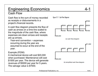
1. Professional Publications, Inc. FERC
4-1Engineering Economics
Cash Flow
Cash flow is the sum of money recorded
as receipts or disbursements in a
project’s financial records.
A cash flow diagram presents the flow of
cash as arrows on a time line scaled to
the magnitude of the cash flow, where
expenses are down arrows and receipts
are up arrows.
Year-end convention ~ expenses
occurring during the year are
assumed to occur at the end of the
year.
Example (FEIM):
A mechanical device will cost $20,000
when purchased. Maintenance will cost
$1000 per year. The device will generate
revenues of $5000 per year for 5 years.
The salvage value is $7000.
2. Professional Publications, Inc. FERC
4-2a1Engineering Economics
Discount Factors and Equivalence
Present Worth (P): present amount at t = 0
Future Worth (F): equivalent future amount at t = n of any present
amount at t = 0
Annual Amount (A): uniform amount that repeats at the end of each
year for n years
Uniform Gradient Amount (G): uniform gradient amount that repeats at
the end of each year, starting at the end of the second year and
stopping at the end of year n.
3. Professional Publications, Inc. FERC
4-2a2Engineering Economics
Discount Factors and Equivalence
NOTE: To save time,
use the calculated
factor table provided
in the NCEES FE
Handbook.
4. Professional Publications, Inc. FERC
4-2bEngineering Economics
Discount Factors and Equivalence
Example (FEIM):
How much should be put in an investment with a 10% effective annual
rate today to have $10,000 in five years?
Using the formula in the factor conversion table,
P = F(1 + i) –n = ($10,000)(1 + 0.1) –5 = $6209
Or using the factor table for 10%,
P = F(P/F, i%, n) = ($10,000)(0.6209) = $6209
5. Professional Publications, Inc. FERC
4-2cEngineering Economics
Discount Factors and Equivalence
Example (FEIM):
What factor will convert a gradient cash flow ending at t = 8 to a future
value? The effective interest rate is 10%.
The F/G conversion is not given in the factor table. However, there are
different ways to get the factor using the factors that are in the table. For
example,
NOTE: The answers arrived at using the formula versus the factor table
turn out to be slightly different. On economics problems, one should not
worry about getting the exact answer.
= (11.4359)(3.0045)
= 34.3592
(F/G,i%,8) = (F/A,10%,8)(A/G,10%,8)
(F/G,i%,8) = (P/G,10%,8)(F/P,10%,8)
= (16.0287)(2.1436)
= 34.3591
or
6. Professional Publications, Inc. FERC
4-3Engineering Economics
Nonannual Compounding
Effective Annual Interest Rate
An interest rate that is compounded more than once in a year is
converted from a compound nominal rate to an annual effective rate.
Effective Interest Rate Per Period
Effective Annual Interest Rate
Example (FEIM):
A savings and loan offers a 5.25% rate per annum compound daily over
365 days per year. What is the effective annual rate?
!
ie = 1+
r
m
"
#
$
%
&
'
m
(1= 1+
0.0525
365
"
#
$
%
&
'
365
(1= 0.0539
7. Professional Publications, Inc. FERC
4-4Engineering Economics
Discount Factors for Continuous Compounding
The formulas for continuous compounding are the same formulas in the
factor conversion table with the limit taken as the number of periods, n,
goes to infinity.
8. Professional Publications, Inc. FERC
4-5aEngineering Economics
Comparison of Alternatives
Present Worth
When alternatives do the same job and have the same lifetimes,
compare them by converting each to its cash value today. The superior
alternative will have the highest present worth.
Example (EIT8):
9. Professional Publications, Inc. FERC
4-5b1Engineering Economics
Comparison of Alternatives
Capitalized Costs
Used for a project with infinite life that has repeating expenses every
year.
Compare alternatives by calculating the capitalized costs (i.e., the
amount of money needed to pay the start-up cost and to yield enough
interest to pay the annual cost without touching the principal).
NOTE: The factor conversion for a project with no end is the limit of the
P/A factor as the number of periods, n, goes to infinity.
11. Professional Publications, Inc. FERC
4-5cEngineering Economics
Comparison of Alternatives
Annual Cost
When alternatives do the same job but have different lives, compare the
cost per year of each alternative.
The alternatives are assumed to be replaced at the end of their lives by
identical alternatives. The initial costs are assumed to be borrowed at
the start and repaid evenly during the life of the alternative.
Example (EIT8):
12. Professional Publications, Inc. FERC
4-5dEngineering Economics
Comparison of Alternatives
Cost-Benefit Analysis
Project is considered acceptable if B – C ≥ 0 or B/C ≥ 1.
Example (FEIM):
The initial cost of a proposed project is $40M, the capitalized perpetual
annual cost is $12M, the capitalized benefit is $49M, and the residual
value is $0. Should the project be undertaken?
B = $49M, C = $40M + $12M + $0
B – C = $49M – $52M = –$3M < 0
The project should not be undertaken.
13. Professional Publications, Inc. FERC
4-5eEngineering Economics
Comparison of Alternatives
Rate of Return on an Investment (ROI)
The ROI must exceed the minimum attractive rate of return (MARR).
The rate of return is calculated by finding an interest rate that makes the
present worth zero. Often this must be done by trial and error.
14. Professional Publications, Inc. FERC
4-6aEngineering Economics
Depreciation
Straight Line Depreciation
The depreciation per year is the cost minus the salvage value divided by
the years of life.
15. Professional Publications, Inc. FERC
4-6bEngineering Economics
Depreciation
Accelerated Cost Recovery System (ACRS)
The depreciation per year is the cost times the ACRS factor (see the
table in the NCEES Handbook). Salvage value is not considered.
16. Professional Publications, Inc. FERC
4-6cEngineering Economics
Depreciation
Example (FEIM):
An asset is purchased that costs $9000. It has a 10-year life and a salvage
value of $200. Find the straight-line depreciation and ACRS depreciation
for 3 years.
Straight-line depreciation/year
ACRS depreciation
First year ($9000)(0.1) = $ 900
Second year ($9000)(0.18) = $1620
Third year ($9000)(0.144) = $1296
!
=
$9000" $200
10
= $880/ yr
17. Professional Publications, Inc. FERC
4-6dEngineering Economics
Depreciation
Book Value
The assumed value of the asset after j years. The book value (BVj) is the
initial cost minus the sum of the depreciations out to the jth year.
Example (FEIM):
What is the book value of the asset in the previous example after 3 years
using straight-line depreciation? Using ACRS depreciation?
Straight-line depreciation
$9000 – (3)($800) = $6360
ACRS depreciation
$9000 – $900 – $1620 – $1296 = $5184
18. Professional Publications, Inc. FERC
4-7aEngineering Economics
Tax Considerations
Expenses and depreciation are deductible, revenues are taxed.
Example (EIT8):
19. Professional Publications, Inc. FERC
4-7bEngineering Economics
Tax Considerations
Tax Credit
A one-time benefit from a purchase that is subtracted from income taxes.
Example (EIT8):
20. Professional Publications, Inc. FERC
4-7cEngineering Economics
Tax Considerations
Gain or loss on the sale of an asset:
If an asset has been depreciated and then is sold for more than the book
value, the difference is taxed.
21. Professional Publications, Inc. FERC
4-8Engineering Economics
Bonds
Bond value is the present worth of payments over the life of the bond.
Bond yield is the equivalent interest rate of the bond compared to the
bond cost.
Example (EIT8):
22. Professional Publications, Inc. FERC
4-9Engineering Economics
Break-Even Analysis
Calculating when revenue is equal to cost, or when one alternative is equal to
another if both depend on some variable.
Example (FEIM):
How many kilometers must a car be driven per year for leasing and buying to cost
the same? Use 10% interest and year-end cost.
Leasing: $0.15 per kilometer
Buying: $5000 purchase cost, 3-year life, salvage $1200,
$0.04 per kilometer for gas and oil, $500 per year for insurance
EUAC (leasing) = $0.15x, where x is kilometers driven
EUAC (buying) = $0.04x + $500 + ($5k)(A/P,10%,3) – ($1.2k)(A/F,10%,3)
= $0.04x + $500 + ($5k)(0.4021) – ($1.2k)(0.3021)
= $0.04x + $2148
Setting EUAC (leasing) = EUAC (buying) and solving for x
$0.15x = $0.04x + $2148
x = 19,527 km must be driven to break even
24. Professional Publications, Inc. FERC
4-11aEngineering Economics
Additional Examples
Example 1 (FEIM):
What is the uninflated present worth of $2000 in 2 years if the average
inflation rate is 6% and i is 10%?
d = i + f + if = 0.06 + 0.10 + (0.06)(0.10) = 0.166
P = ($2000)(P/F,16.6%,2) = ($2000)(1 + d)–n
= ($2000)(1 + 0.166)–2 = $1471
25. Professional Publications, Inc. FERC
4-11bEngineering Economics
Additional Examples
Example 2 (FEIM):
It costs $75 per year to maintain a cemetery plot. If the interest rate is
6.0%, how much must be set aside to pay for maintenance on each plot
without touching the principal?
(A) $1150
(B) $1200
(C) $1250
(D) $1300
P = ($75)(P/A,6%,∞) = ($75)(1/0.06) = $1250
Therefore, (C) is correct.
26. Professional Publications, Inc. FERC
4-11cEngineering Economics
Additional Examples
Example 3 (FEIM):
It costs $1000 for hand tools and $1.50 labor per unit to manufacture a
product. Another alternative is to manufacture the product by an
automated process that costs $15,000, with a $0.50 per-unit cost. With
an annual production rate of 5000 units, how long will it take to reach the
break-even point?
(A) 2.0 yr
(B) 2.8 yr
(C) 3.6 yr
(D) never
Cumulative cost (hand tools) = $1000 + $1.50x, where x is the number
of units.
Cumulative cost (automated) = $15,000 + $0.50x
Set cumulative costs equal and solve for x.
$1000 + $1.50x = $15,000 + $0.50x
$1x = $14,000
x = 14,000 units
tbreak-even = x/production rate = 14,000/5000 = 2.8 yr
Therefore, (B) is correct.
27. Professional Publications, Inc. FERC
4-11dEngineering Economics
Additional Examples
Example 4 (FEIM):
A loan of $10,000 is made today at an interest rate of 15%, and the first
payment of $3000 is made 4 years later. The amount that is still due on
the loan after the first payment is most nearly
(A) $7000
(B) $8050
(C) $8500
(D) $14,500
loan due = ($10k)(F/P,15%,4) – $3000
= ($10k)(1 + 0.15)4 – $3000
= ($10k)(1.7490) – $3000
= $14,490 ($14,500)
Therefore, (D) is correct.
28. Professional Publications, Inc. FERC
4-11eEngineering Economics
Additional Examples
Example 5 (FEIM):
A machine is purchased for $1000 and has a useful life of 12 years. At
the end of 12 years, the salvage value is $130. By straight-line
depreciation, what is the book value of the machine at the end of 8
years?
(A) $290
(B) $330
(C) $420
(D) $580
BV = $1000 – ($1000 – $130)(8/12) = $1000 – $580 = $420
Therefore, (C) is correct.
29. Professional Publications, Inc. FERC
4-11fEngineering Economics
Additional Examples
Example 6 (FEIM):
The maintenance cost for an investment is $2000 per year for the first 10
years and $1000 per year thereafter. The investment has infinite life.
With a 10% interest rate, the present worth of the annual disbursement is
most nearly
(A) $10,000
(B) $16,000
(C) $20,000
(D) $24,000
The costs or benefits for a cash flow that repeat should be broken into
different benefits and costs that all start or finish at the time of interest.
Take the $2000 cost that repeats for 10 years and break it into two
$1000 costs to have one $1000 cost that goes on infinitely and one
$1000 cost that goes on for 10 years.
P = ($1000)(P/A,10%,10) + ($1000)(P/A,10%,∞)
= ($1000)(6.1446) + ($1000)(1/0.10)
= $6144.6 + $10,000 = $16,144.6 ($16,000)
Therefore, (B) is correct.
30. Professional Publications, Inc. FERC
4-11gEngineering Economics
Additional Examples
Example 7 (FEIM):
With an interest rate of 8% compounded semiannually, the value of a
$1000 investment after 5 years is most nearly
(A) $1400
(B) $1470
(C) $1480
(D) $1800
ie = (1 + r/m)m – 1= (1 + 0.08/2)2 – 1 = 0.0816
F = ($1000)(F/P,8.16%,5) = ($1000)(1 + 0.0816)5
= ($1000)(1.480) = $1480
Therefore, (C) is correct.
31. Professional Publications, Inc. FERC
4-11h1Engineering Economics
Additional Examples
Example 8 (FEIM):
The following data applies for example problems 8.1 through 8.3. A company is
considering the purchase of either machine A or machine B.
machine A machine B
initial cost $80,000 $100,000
estimated life 20 years 25 years
salvage value $20,000 $25,000
other costs $18,000 per year $15,000 per year for the first 15 years
$20,000 per year for the next 10 years
Example 8.1 (FEIM):
The interest rate is 10%, and all cash flows may be treated as end-of-year cash
flows. Assume that equivalent annual cost is the value of the constant annuity
equal to the total cost of a project. The equivalent annual cost of machine B is
most nearly
(A) $21,000
(B) $21,500
(C) $23,000
(D) $26,500
32. Professional Publications, Inc. FERC
4-11h2Engineering Economics
Additional Examples
The $15,000 cost for 15 years and the $20,000 cost for the next 10 years
can be broken into a $20,000 cost for the full 25 years and a $5000 benefit
that is present for the first 15 years.
The present worth of $20k for 25 years is
P($20,25) = ($20k)(P/A,10%,25) = ($20k)(9.0770) = $181.54k
The present worth of $5k for 15 years is
P($5,15) = ($5k)(P/A,10%,15) = ($5k)(7.6061) = 38.03k
Pother costs = $181.54 k + $38.03k = $143.51k
Aother costs = Pother costs(A/P, 10%, 25) = ($143.51k)(0.1102) = $15,815
EUAC = ($100k)(A/P,10%,25) – ($25k)(A/F,10%,25) + $15,815
= ($100k)(0.1102) – ($25k)(0.0102) + $15,815
= $11,020 – $255 + $15,815 = $26,610 ($26,500)
Therefore, (D) is correct.
33. Professional Publications, Inc. FERC
4-11h3Engineering Economics
Additional Examples
Example 8.2 (FEIM):
If funds equal to the present worth of the cost of purchasing and using
machine A over 20 years were invested at 10% per annum, the value of
the investment at the end of 20 years would be most nearly:
(A) $548,000
(B) $676,000
(C) $880,000
(D) $1,550,000
P(A) = $80k + ($20k)(P/F,10%,20) – ($18k)(P/A,10%,20)
= $80k + ($20k)(0.1486) – ($18k)(8.5136)
= $80k + $2.972k – $153.245k
= $230,273
F(A,10%,20) = ($230,273)(F/P,10%,20) = ($230,273)(6.7275)
= $1,549,162 ($1,550,000)
Therefore, (D) is correct.
34. Professional Publications, Inc. FERC
4-11h4Engineering Economics
Additional Examples
Example 8.3 (FEIM):
How much money would have to be placed in a sinking fund each year to
replace machine B at the end of 25 years if the fund yields 10% annual
compound interest and if the first cost of the machine is assumed to
increase at a 6% annual compound rate? (Assume the salvage value does
not change.)
(A) $2030
(B) $2510
(C) $2540
(D) $4110
F = P(F/P,6%,25) – salvage value = ($100,000)(4.2919) – $25,000
= $404,190
A = F(A/F,10%,25) = ($404,190)(0.0102)
= $4123 ($4110)
Therefore, (D) is correct.