This document describes the design and analysis of a quarter-wave transmission line and a single-stub transmission line. It provides the initial parameters and equations used to design the transmission lines. Graphs of standing wave ratio (SWR) versus normalized frequency are generated for each type of transmission line using MATLAB. The bandwidths of the transmission lines are then calculated and compared based on the SWR graphs. Key findings include the quarter-wave transmission line having a more consistent SWR and bandwidth, while the single-stub transmission line has a higher chance of fully reflecting signals back to the generator.

1. Transmission Line Design:
Quarter-Wave
&
Single-Stub
Applied Electromagnetic Waves ECE 3317
Professor Chen
Julia London
Spring 2014

2. London 2
Table of Contents
I. Abstract........................................................................................................................................ 3
II. Introduction................................................................................................................................ 4
III. Analysis and Design.................................................................................................................. 4
Quarter-Wave Transformer......................................................................................................... 4
Figure 1 – QWT Initial Design................................................................................................ 5
Table 1 – Initial Givens for Transmission Lines ..................................................................... 5
Figure 2 – QWT Final Design ................................................................................................. 6
Short-Stub Transmission Line..................................................................................................... 7
Figure 3 – SST Initial Design.................................................................................................. 7
Figure 4 – Solution for d.......................................................................................................... 9
Figure 5 – SST Final Design ................................................................................................. 10
IV. Results..................................................................................................................................... 11
Quarter-Wave Transmission Line ............................................................................................. 11
Figure 6 – QWT SWR vs.
𝐟
𝐟 𝟎
.................................................................................................. 12
Figure 7 – QWT SWR vs.
𝐟
𝐟 𝟎
Extended.................................................................................. 13
Table 2 – QWT Varying Bandwidth ..................................................................................... 14
Single-Stub Transmission Line ................................................................................................. 14
Figure 8 – SST SWR vs.
𝐟
𝐟 𝟎
.................................................................................................... 15
Figure 9 – SST SWR vs.
𝐟
𝐟 𝟎
Extended .................................................................................... 16
Table 3 – SST Varying Bandwidth........................................................................................ 17
V. Conclusions.............................................................................................................................. 18
VI. References............................................................................................................................... 19

3. London 3
I. Abstract
A problem in designing an effective quarter-wave transmission line and a single-stub
transmission line was presented towards the middle of the semester. After designing said
transmission lines the second task was to observe the change in their standing wave ratios due to
the change in their normalized frequencies. Once this was observed, the percent bandwidths of
both types of transmission lines were to be recorded and compared, along with their standing
wave ratio relationships.
Using MATLAB, several derived equations and allowing the single-stub transmission
line to have a short circuit stub, both graphs were plotted and recorded in increments of 1[MHz].
Through observation, it was noted that the quarter-wave transmission line had a more consistent
change in SWR and bandwidth than the single-stub transmission line. It was also noted that the
single-stub had a higher chance of reflecting an entire signal back to the generator than actually
allowing the load to absorb the signal. Although the bandwidth for the quarter-wave transmission
line at first appeared to have been too large for the analysis, through further research it was
confirmed that the bandwidth was a reasonable amount for the stated initial frequency.

4. London 4
II. Introduction
Transmission lines are used to transmit the alternating currents of radio frequencies. Such
signals operate on such high enough frequencies that they must be taken into account; otherwise
the transmission would be lost. Transmission lines are also used in everyday life from
distributing cable television to network connection for high-speed computers. Different
transmission lines range from coaxial cables to optical fibers, but the transmission line that will
be discussed is the losses transmission line in two forms, quarter-wave (QWT) and single-stub
(SST). With these two types of transmission lines a graph will be generated to see how the
change in frequency will relate to their relative Standing Wave Ratios (SWR). The standing
wave ratio is the ratio between the highest amplitude of the single versus its lowest amplitude.
This ratio is used to determine the efficiency of a transmission line with SWR being equal to 1 as
the most idea transmission line, and SWR being equal to infinity being the most inefficient. Once
the SWR graphs have been generated their relative bandwidths will be noted and compared.
III. Analysis and Design
Quarter-Wave Transformer
Below in Figure 1 is the set up for a quarter wave transmission line.

5. London 5
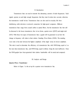
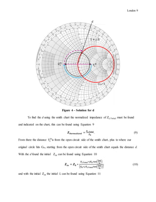
Figure 1 – QWT Initial Design
Before being able to generate a SWR vs. the normalized frequency graph some initial conditions
must be built into the transmission line.
Below in Table 1 is the initial conditions given for the project.
Table 1 – Initial Givens for Transmission Lines
Givens
𝒁 𝟎 75 [Ω]
𝒁 𝑳 75 [Ω]
𝒁 𝟎𝒔 75 [Ω]
c 3x108 [m/s]
Knowing this we can calculate the initial length, 𝑙, lambda, 𝜆0, Z0T, stub-length,𝑙 𝑠, and stub
impedance. Because this is a quarter-wave transmission line the stub impedance is unnecessary
thus making the stub length and its impedance equal to zero. Next the initial lambda can be
found by using Equation 1
𝜆0 = 𝑐/𝑓0 , (1)
𝑍0 𝑍0𝑇 𝑍 𝐿
𝑍0𝑠
𝑙
𝑙 𝑠
𝑍 𝐿
𝑍𝑖𝑛
𝑍0
𝑍0

6. London 6
With f0 as an initial frequency and c equal to the speed of light. For this project f0 and c will be
equal, simply to aid in the ease of generating the SWR graph.
Once the initial lambda has been found the initial distance that Z0T will be affecting can
be found with Equation 2,
𝒍 = 𝝀 𝟎/𝟒. (2)
Next the impedances were calculated. Initially the load has two impedances that are in
parallel, these impedances can be combined. Because the wires connecting the impedances have
the same resistance the impedances can be combined into one by using Equation 3
𝒁 𝑳 𝑻𝒐𝒕𝒂𝒍 =
𝟏
𝟏
𝒁 𝑳
+
𝟏
𝒁 𝑳
, (3)
and Z0T can be found by using Equation 4
𝒁 𝟎𝑻 = √ 𝒁 𝟎 ∗ 𝒁 𝑳 𝑻𝒐𝒕𝒂𝒍. (4)
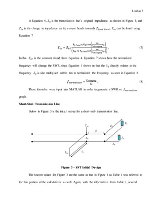
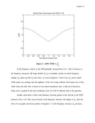
The final layout for the quarter wave transmission line can be seen in Figure 2
Figure 2 – QWT Final Design
Now that the initial conditions have been found the changing aspects of the transmission
line, due to the change in frequency, can be found.
To find how frequency relates to SWR Equation 5
𝑺𝑾𝑹 =
𝟏+| 𝜞|
𝟏−| 𝜞|
, (5)
is used, where Γ is found using Equation 6
𝚪 =
𝒁 𝒊𝒏−𝒁 𝟎
( 𝒁 𝒊𝒏+𝒁 𝟎)
, (6)
𝑍0 = 75[Ω] 𝑍0𝑇 = 53.33 [Ω] 𝑍 𝐿 𝑇𝑜𝑡𝑎𝑙 = 37.5 [Ω]
𝑙 = .25𝜆 [𝑚]

7. London 7
In Equation 6, 𝑍0 is the transmission line’s original impedance, as shown in Figure 1, and
𝑍𝑖𝑛 is the change in impedance as the current heads towards 𝑍 𝐿𝑜𝑎𝑑 𝑇𝑜𝑡𝑎𝑙 . 𝑍𝑖𝑛 can be found using
Equation 7
𝒁𝒊𝒏 = 𝒁 𝟎𝑻
𝒁 𝑳 𝑻𝒐𝒕𝒂𝒍+𝒋𝒁 𝟎𝑻 𝐭𝐚𝐧(
𝟐𝝅𝒍
𝝀 𝒄𝒉𝒂𝒏𝒈𝒊𝒏𝒈
𝝀 𝟎 )
( 𝒁 𝟎𝑻 +𝒋 𝒁 𝑳 𝑻𝒐𝒕𝒂𝒍 𝐭𝐚𝐧(
𝟐𝝅𝒍
𝝀 𝒄𝒉𝒂𝒏𝒈𝒊𝒏𝒈
𝝀 𝟎 ))
, (7)
In this 𝑍0𝑇 is the constant found from Equation 4. Equation 7 shows how the normalized
frequency will change the SWR, since Equation 1 shows us that the 𝜆0 directly relates to the
frequency. 𝜆0 is also multiplied within tan to normalized the frequency, as seen in Equation 8
𝒇 𝒏𝒐𝒓𝒎𝒂 𝒍𝒊𝒛𝒆𝒅 =
𝒇 𝒄𝒉𝒂𝒏𝒈𝒊𝒏𝒈
𝒇 𝟎
. (8)
These formulae were input into MATLAB in order to generate a SWR vs. 𝑓𝑛𝑜𝑟𝑚𝑎𝑙𝑖𝑧𝑒𝑑
graph.
Short-Stub Transmission Line
Below in Figure 3 is the initial set up for a short-stub transmission line.
Figure 3 – SST Initial Design
The known values for Figure 3 are the same as that in Figure 1 so Table 1 was referred to
for this portion of the calculations as well. Again, with the information from Table 1, several
𝑍0 𝑍 𝐿
𝑍0𝑠
𝑑
𝑙 𝑠
𝑍 𝐿
𝑍𝑖𝑛
𝑍0
𝑍0

8. London 8
unknowns can be found for Figure 2. These unknowns include the distance the stub is away from
the load, 𝑑, the stub length, 𝑙 𝑠, and the impedance of the stub, 𝑗𝛽𝑠𝑡𝑢𝑏.
Again, as was done for Figure 1 the load impedances can be combined using Equation 3.
To simplify the problem 𝜆0, used for the quarter-wave transmission, line will be used for these
calculations. Knowing the new load impedance 𝑑 can be found using a smith chart,
corresponding to whether the stub is an open or short circuit. For the following calculations the
stub is a short circuit.
Figure 4 shows the solution for 𝑑 with the stub as a short circuit. 𝑍 𝐿
𝑁
Represents the
normalized load impedance, 𝑌𝐿
𝑁
represents the normalized load admittance and 𝑑 represents the
𝑑 for Figure 3.

9. London 9
Figure 4 – Solution for d
To find the d using the smith chart the normalized impedance of 𝑍 𝐿 𝑇𝑜𝑡𝑎𝑙 must be found
and indicated on the chart, this can be found using Equation 9
𝒁 𝑵𝒐𝒓𝒎𝒂𝒍𝒊𝒛𝒆𝒅 =
𝒁 𝑳 𝑻𝒐𝒕𝒂𝒍
𝒁 𝟎
. (9)
From there the distance 𝑌𝐿
𝑁
is from the open circuit side of the smith chart, plus to where our
original circle hits Gin, starting from the open circuit side of the smith chart equals the distance d.
With the d found the initial 𝑍𝑖𝑛 can be found using Equation 10
𝒁𝒊𝒏 = 𝒁 𝟎 ∗
𝒁 𝑳 𝑻𝒐𝒕𝒂𝒍+𝒋𝒁 𝟎 𝒕𝒂𝒏(
𝟐𝝅𝒅
𝝀 𝟎
)
( 𝒁 𝟎+𝒋 𝒁 𝑳 𝑻𝒐𝒕𝒂𝒍 𝒕𝒂𝒏(
𝟐𝝅𝒅
𝝀 𝟎
))
, (10)
and with the initial 𝑍𝑖𝑛 the initial ls can be found using Equation 11
𝑌𝐿
𝑁
Gin=1
1 + 𝑗. 8
𝑑
𝑍 𝐿
𝑁

10. London 10
𝒍 𝒔 =
𝒄𝒐𝒕−𝟏( 𝑰𝒎{ 𝟏/𝒁 𝒊𝒏}∗𝒁 𝟎) 𝝀 𝟎
𝟐𝝅
. (11)
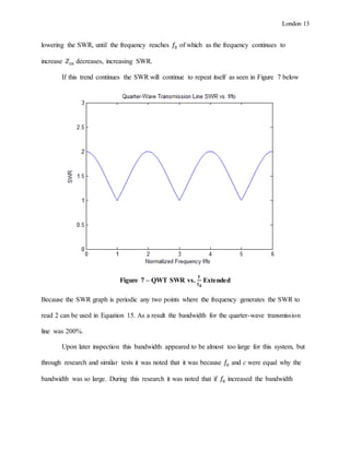
Now that all the initial conditions have been found several equations were derived in
order to relate the change in the normalized frequency to SWR, and the final set up for Figure 3
can be seen in Figure 5
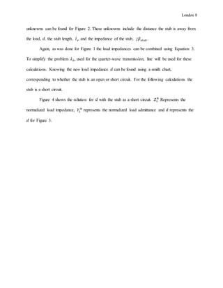
Figure 5 – SST Final Design
From Equations 5 and 6 it can be noted that 𝑍𝑖𝑛will affect SWR and from Equation 10 it
can be noted that 𝑍𝑖𝑛 is directly affected by the changing frequency. With this knowledge
Equation 12 can be derived
𝑍𝑖𝑛 = 𝑍0
𝑍 𝐿 𝑇𝑜𝑡𝑎𝑙 +𝑗𝑍0 tan(
2𝜋𝑑
𝜆 𝐶ℎ𝑎𝑛𝑔𝑖𝑛𝑔
𝜆0)
( 𝑍0 +𝑗 𝑍 𝐿 𝑇𝑜𝑡𝑎𝑙 tan(
2𝜋𝑑
𝜆 𝐶ℎ𝑎𝑛𝑔𝑖𝑛𝑔
𝜆0))
. (12)
Because the impedance of the stub is, at 𝑓0 , supposed to cancel out the imaginary portion of the
admittance of 𝑍𝑖𝑛 so that 𝑍𝑖𝑛 matches 𝑍0 Equation 13 can be derived from Equation 12 to solve
for the stub’s admittance
𝑗𝛽𝑠𝑡𝑢𝑏 = −
𝑗
𝑍0𝑠 tan(
2𝜋
𝜆 𝐶ℎ𝑎𝑛𝑔𝑖𝑛𝑔
𝜆0 𝑙 𝑠)
. (13)
As seen in Figure 3 it can be noted that the stub impedance and 𝑍𝑖𝑛 are in parallel, thus to find
the new 𝑍𝑖𝑛, that can be used in Equation 6, Equation 14 was derived from Equation 3
𝑍0 = 75 [Ω] 𝑍 𝐿 𝑇𝑜𝑡𝑎𝑙 = 37.5 [Ω]
𝑍0𝑠 = 75 [Ω]
𝑑 = .402𝜆 [𝑚]
𝑙 𝑠 = .152𝜆 [𝑚]
𝑍𝑖𝑛
𝑍0 = 75[Ω]

11. London 11
𝑍𝑖𝑛 𝑛𝑒𝑤 =
1
𝑗𝛽+
1
𝑍 𝑖𝑛
. (14)
In MATLAB 𝑍𝑖𝑛 𝑛𝑒𝑤 can be input into Equation 6 which will be used in Equation 5 to generate
the different SWRs for each frequency.
To allow MATLAB to not over flow with information the changing frequency ranges
from zero to 600 [MHz], which will be plotted in intervals of 1 [MHz] Once the SWR graphs
have been created the bandwidths of both the quarter-wave and single-stub transmission lines
will be calculated using Equation 15
𝐵𝑎𝑛𝑑𝑤𝑖𝑑𝑡ℎ =
| 𝑓2−𝑓1|
𝑓0
100%. (15)
𝑓2 and 𝑓1are the frequencies, one immediately after each other, where the Standing Wave Ratio
equals 2.
IV. Results
Quarter-Wave Transmission Line
Figure 5 displays the SWR vs. the normalized frequency for the quarter wave
transmission line.

12. London 12
Figure 6 – QWT SWR vs.
𝐟
𝐟 𝟎
As the frequency neared 𝑓0 the SWR gradually decayed from 2 to 1. This is because as
the frequency increased, still being divided by 𝑓0, it eventually reaches its match frequency,
making 𝑍𝑖𝑛 match up with 𝑍0 once more. As seen in Equations 5 and 6 once 𝑍𝑖𝑛 and 𝑍0 match
SWR equals one, meaning that the amplitude of the wave being reflected back equals zero of that
which enters the load. This is known to be an ideal transmission line, in that all of the power
being sent is acquired by the load considering none of it will be reflected back to the generator.
Another observation is that as the frequency becomes greater or less that the 𝑓0 the SWR
increases from 1 to 2. This occurs because as the frequency increases the change in 𝑍𝑖𝑛 takes the
form of a sin graph, due the tan portion of Equation 7. As the frequency increases 𝑍𝑖𝑛 increases,

13. London 13
lowering the SWR, until the frequency reaches 𝑓0 of which as the frequency continues to
increase 𝑍𝑖𝑛 decreases, increasing SWR.
If this trend continues the SWR will continue to repeat itself as seen in Figure 7 below
Figure 7 – QWT SWR vs.
𝐟
𝐟 𝟎
Extended
Because the SWR graph is periodic any two points where the frequency generates the SWR to
read 2 can be used in Equation 15. As a result the bandwidth for the quarter-wave transmission
line was 200%.
Upon later inspection this bandwidth appeared to be almost too large for this system, but
through research and similar tests it was noted that it was because 𝑓0 and c were equal why the
bandwidth was so large. During this research it was noted that if 𝑓0 increased the bandwidth

14. London 14
would decrease and if 𝑓0 would decrease the bandwidth would increase. The trend of increasing
𝑓0 can be seen in Table 2 below.
Table 2 – QWT Varying Bandwidth
Varying Bandwidth
𝒇 𝟎 Bandwidth
400 [MHz] 150 [%]
500 [MHz] 120 [%]
600 [MHz] 100 [%]
700 [MHz] 85.714 [%]
800 [MHz] 75 [%]
For this transmission line lowering 𝑓0 below the value of c would result in an unfeasible
bandwidth considering that “the theoretical limit for percent bandwidth is 200%” (Wikipedia 4).
After considering these observations the bandwidth calculations were determined to be valid.
Single-Stub Transmission Line
Figure 8 displays the zoomed in version of the SWR vs. the normalized frequency graph
for the single-stub transmission line.

15. London 15
Figure 8 – SST SWR vs.
𝐟
𝐟 𝟎
For a reasonable graph to be shown boundaries had to be set for the SWR. This is
because of how a zero frequency affects 𝑍𝑖𝑛 and 𝑗𝛽𝑠𝑡𝑢𝑏. Imputing zero for 𝜆 𝐶ℎ𝑎𝑛𝑔𝑖𝑛𝑔 into
Equations 12 and 13 cancels out tan portion of the equation resulting in 𝑗𝛽𝑠𝑡𝑢𝑏to equal infinity
and 𝑍𝑖𝑛 to equal 𝑍 𝐿 𝑇𝑜𝑡𝑎𝑙 . With an incredibly large imaginary impedance, 𝑍𝑖𝑛 𝑛𝑒𝑤 becomes very
small resulting in Γ being equal to one, thus generating an infinite SWR. An infinite SWR is the
exact opposite of a zero SWR; it means that all the power transmitted to a load has been reflected
back. This makes sense since the stub is a short circuit, making it so that most if not all the
current going through the transmission line will go through the short rather than the load. This is
not the best result considering an ideal reflection is when no power has been returned to the
generator, and all of it has been absorbed by the load.

16. London 16
Another graph was generated to see the change in SWR as frequency increased. Figure 9
displays the SWR vs. the normalized frequency with the last frequency three times the amount of
the original end frequency
Figure 9 – SST SWR vs.
𝐟
𝐟 𝟎
Extended
From Figure 9 it can be noted that the SWR graph for a single-stub transmission line is
not periodic like the quarter-wave transformer. This is probably because not only is the graph
affected by the tangent of 𝑍𝑖𝑛 it is also affected by the tangent in 𝑗𝛽𝑠𝑡𝑢𝑏. Because the periods of
these two equations do not divide rationally they simply cannot form a periodic function, thus
not allowing for a consistent bandwidth.
After analyzing the graphs Figure 8 was used to determine the bandwidth of the single-
stub transmission line. To simplify the calculation the two frequencies closest to 𝑓0that equaled 2

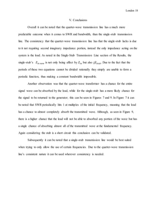
17. London 17
were used in Equation 15. The determined bandwidth of the transmission line was 35.667%, but
this bandwidth was not constant throughout the graph. Several other points were used to
calculate the bandwidth; the results can be seen in Table 3
Table 3 – SST Varying Bandwidth
Bandwidth
Frequencies [MHz]
(𝒇 𝟏𝒇 𝟐)
Bandwidth [%]
259  366 35.667
366  491 41.667
491  492 .333
492  493 .333
493  494 .333
494  548 18
548  549 .333
549  779 76.667
By observing Figure 9 and Table 3 it can be expected that the bandwidth will not become
a constant trend as long as the frequency continues to increase.
Though the data for both the quarter-wave and single-stub transmission lines were not
plotted out in increments of one hertz the data for both graphs seem valid. The outcomes of both
transmission lines were justified by prior knowledge, outside resources and equation analysis.

18. London 18
V. Conclusions
Overall it can be noted that the quarter-wave transmission line has a much more
predictable outcome when it comes to SWR and bandwidth, than the single-stub transmission
line. The consistency that the quarter-wave transmission line has that the single-stub lacks is due
to it not requiring second imaginary impedance portion, instead the only impedance acting on the
system is the load. As noted in the Single-Stub Transmission Line section of the Results, the
single-stub’s 𝑍𝑖𝑛 𝑛𝑒𝑤 is not only being affect by 𝑍𝑖𝑛 but also 𝑗𝛽𝑠𝑡𝑢𝑏. Due to the fact that the
periods of these two equations cannot be divided rationally they simply are unable to form a
periodic function, thus making a constant bandwidth impossible.
Another observation was that the quarter-wave transformer has a chance for the entire
signal wave can be absorbed by the load, while for the single-stub has a more likely chance for
the signal to be returned to the generator; this can be seen in Figures 7 and 9. In Figure 7 it can
be noted that SWR periodically hits 1 at multiples of the initial frequency, meaning that the load
has a chance to almost completely absorb the transmitted wave. Although, as seen in Figure 9,
there is a higher chance that the load will not be able to absorbed any portion of the wave but has
a single chance of absorbing almost all of the transmitted wave at the fundamental frequency.
Again considering the stub is a short circuit this conclusion can be validated.
Subsequently it can be noted that a single-stub transmission line would be best suited
when trying to only allow the use of certain frequencies. Due to the quarter-wave transmission
line’s consistent nature it can be used wherever consistency is needed.

19. London 19
VI. References
[1] Professor Chen. 2014. Transmission Lines (Impedance Matching) Notes 13. Available
http://www0.egr.uh.edu/courses/ECE/ECE3317/SectionChen/Class%20Notes/
[2] Stiles, J. 2014. 5.2 – Single-Stub Tuning [Online]. Available FTP:
http://www.ittc.ku.edu/~jstiles/723/handouts/section_5_2_Single_Stub_Tuning_p
ackage.pdf
[3] Wikipedia. 2014. Transmission Lines [Online]. Available FTP:
http://en.wikipedia.org/wiki/Transmission_line
[4] Wikipedia. 2014. Bandwidth (Signal Processing) [Online]. Available FTP:
http://en.wikipedia.org/wiki/Bandwidth_(signal_processing)
[5] Donohoe, J. Patrick. 2014. Impedance Matching and Transformation [Online]. Available
FTP: http://www.ece.msstate.edu/~donohoe/ece4333notes5.pdf
[6] Wikipedia. 2014. Quarter-wave Impedance Transformer [Online]. Available FTP:
http://en.wikipedia.org/wiki/Quarter-wave_impedance_transformer
[7] Chew, C.W..2014. Impedance Matching on Transmission Line ECE 350 Lecture Notes
[Online]. Available FTP: http://wcchew.ece.illinois.edu/chew/ece350/ee350-
10.pdf
[8] Bevelacqua, Peter. 2014. VSWR (Voltage Standing Wave Ratio) [Online]. Available FTP:
http://www.antenna-theory.com/definitions/vswr.php