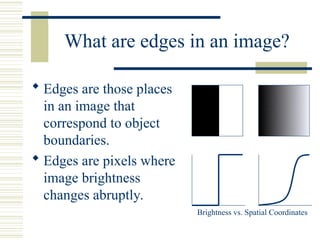
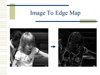
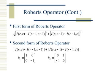
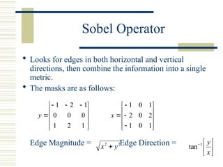
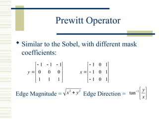
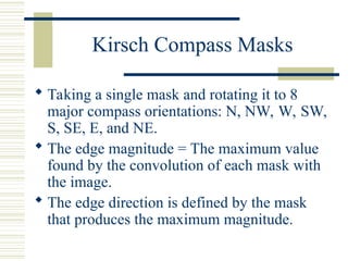
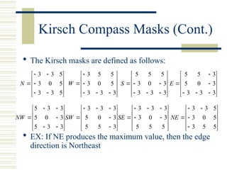
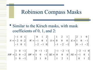
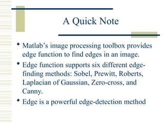
Edge Detection
Hao Huy Tran
Computer Graphics and Image Processing
CIS 581 – Fall 2002
Professor: Dr. Longin Jan Latecki
Edge Detection
• What are edges in an image?
• Edge Detection
• Edge Detection Methods
• Edge Operators
• Matlab Program
• Performance
What are edges in an image?
 Edges are those places
in an image that
correspond to object
boundaries.
 Edges are pixels where
image brightness
changes abruptly.
Brightness vs. Spatial Coordinates
More About Edges
 An edge is a property attached to an
individual pixel and is calculated from the
image function behavior in a neighborhood
of the pixel.
 It is a vector variable (magnitude of the
gradient, direction of an edge) .
 More information about edges can be found
in Dr. Latecki’s Lecture on Filter.
Image To Edge Map
Edge Detection
 Edge information in an image is found by looking
at the relationship a pixel has with its
neighborhoods.
 If a pixel’s gray-level value is similar to those
around it, there is probably not an edge at that
point.
 If a pixel’s has neighbors with widely varying gray
levels, it may present an edge point.
Edge Detection Methods
 Many are implemented with convolution
mask and based on discrete approximations
to differential operators.
 Differential operations measure the rate of
change in the image brightness function.
 Some operators return orientation
information. Other only return information
about the existence of an edge at each point.
Roberts Operator
 Mark edge point only
 No information about edge orientation
 Work best with binary images
 Primary disadvantage:
 High sensitivity to noise
 Few pixels are used to approximate the gradient
Roberts Operator (Cont.)
 First form of Roberts Operator
 Second form of Roberts Operator
   2
2
)
,
1
(
)
1
,
(
)
1
,
1
(
)
,
( c
r
I
c
r
I
c
r
I
c
r
I 






|
)
,
1
(
)
1
,
(
|
|
)
1
,
1
(
)
,
(
| c
r
I
c
r
I
c
r
I
c
r
I 














1
0
0
1
1
h 







0
1
1
0
2
h
Sobel Operator
 Looks for edges in both horizontal and vertical
directions, then combine the information into a single
metric.
 The masks are as follows:
Edge Magnitude = Edge Direction =









 



1
2
1
0
0
0
1
2
1
y














1
0
1
2
0
2
1
0
1
x
2
2
y
x  






x
y
1
tan
Prewitt Operator
 Similar to the Sobel, with different mask
coefficients:
Edge Magnitude = Edge Direction =









 



1
1
1
0
0
0
1
1
1
y














1
0
1
1
0
1
1
0
1
x
2
2
y
x  






x
y
1
tan
Kirsch Compass Masks
 Taking a single mask and rotating it to 8
major compass orientations: N, NW, W, SW,
S, SE, E, and NE.
 The edge magnitude = The maximum value
found by the convolution of each mask with
the image.
 The edge direction is defined by the mask
that produces the maximum magnitude.
Kirsch Compass Masks (Cont.)
 The Kirsch masks are defined as follows:
 EX: If NE produces the maximum value, then the edge
direction is Northeast
















5
3
3
5
0
3
5
3
3
N
















3
3
3
5
0
3
5
5
3
W
















3
3
3
3
0
3
5
5
5
S
















3
3
3
3
0
5
3
5
5
E
















3
3
5
3
0
5
3
3
5
NW
















3
5
5
3
0
5
3
3
3
SW
















5
5
5
3
0
3
3
3
3
SE















5
5
3
5
0
3
5
3
3
NE
Robinson Compass Masks
 Similar to the Kirsch masks, with mask
coefficients of 0, 1, and 2:














1
0
1
2
0
2
1
0
1
N














0
1
2
1
0
1
2
1
0
W














1
2
1
0
0
0
1
2
1
S














2
1
0
1
0
1
0
1
2
E














1
0
1
2
0
2
1
0
1
NW














0
1
2
1
0
1
2
1
0
SW









 



1
2
1
0
0
0
1
2
1
SE














2
1
0
1
0
1
0
1
2
NE
Laplacian Operators
 Edge magnitude is approximated in digital
images by a convolution sum.
 The sign of the result (+ or -) from two
adjacent pixels provide edge orientation and
tells us which side of edge brighter
Laplacian Operators (Cont.)
 Masks for 4 and 8 neighborhoods
 Mask with stressed significance of the
central pixel or its neighborhood














0
1
0
1
4
1
0
1
0


















1
1
1
1
8
1
1
1
1














1
2
1
2
4
2
1
2
1














2
1
2
1
4
1
2
1
2
Edge Map In Matlab Program
 Implement all methods in this presentation
 Set up edge detection mask(s)
 Use convolution method (filter2 function)
 Calculate edge magnitude
 Show the result of edge map
 No calculation of edge direction
Performance
 Sobel and Prewitt methods are very
effectively providing good edge maps.
 Kirsch and Robinson methods require more
time for calculation and their results are not
better than the ones produced by Sobel and
Prewitt methods.
 Roberts and Laplacian methods are not very
good as expected.
A Quick Note
 Matlab’s image processing toolbox provides
edge function to find edges in an image.
 Edge function supports six different edge-
finding methods: Sobel, Prewitt, Roberts,
Laplacian of Gaussian, Zero-cross, and
Canny.
 Edge is a powerful edge-detection method

Edge detection techniques in image processing

  • 1.
    Edge Detection Hao HuyTran Computer Graphics and Image Processing CIS 581 – Fall 2002 Professor: Dr. Longin Jan Latecki
  • 2.
    Edge Detection • Whatare edges in an image? • Edge Detection • Edge Detection Methods • Edge Operators • Matlab Program • Performance
  • 3.
    What are edgesin an image?  Edges are those places in an image that correspond to object boundaries.  Edges are pixels where image brightness changes abruptly. Brightness vs. Spatial Coordinates
  • 4.
    More About Edges An edge is a property attached to an individual pixel and is calculated from the image function behavior in a neighborhood of the pixel.  It is a vector variable (magnitude of the gradient, direction of an edge) .  More information about edges can be found in Dr. Latecki’s Lecture on Filter.
  • 5.
  • 6.
    Edge Detection  Edgeinformation in an image is found by looking at the relationship a pixel has with its neighborhoods.  If a pixel’s gray-level value is similar to those around it, there is probably not an edge at that point.  If a pixel’s has neighbors with widely varying gray levels, it may present an edge point.
  • 7.
    Edge Detection Methods Many are implemented with convolution mask and based on discrete approximations to differential operators.  Differential operations measure the rate of change in the image brightness function.  Some operators return orientation information. Other only return information about the existence of an edge at each point.
  • 8.
    Roberts Operator  Markedge point only  No information about edge orientation  Work best with binary images  Primary disadvantage:  High sensitivity to noise  Few pixels are used to approximate the gradient
  • 9.
    Roberts Operator (Cont.) First form of Roberts Operator  Second form of Roberts Operator    2 2 ) , 1 ( ) 1 , ( ) 1 , 1 ( ) , ( c r I c r I c r I c r I        | ) , 1 ( ) 1 , ( | | ) 1 , 1 ( ) , ( | c r I c r I c r I c r I                1 0 0 1 1 h         0 1 1 0 2 h
  • 10.
    Sobel Operator  Looksfor edges in both horizontal and vertical directions, then combine the information into a single metric.  The masks are as follows: Edge Magnitude = Edge Direction =               1 2 1 0 0 0 1 2 1 y               1 0 1 2 0 2 1 0 1 x 2 2 y x         x y 1 tan
  • 11.
    Prewitt Operator  Similarto the Sobel, with different mask coefficients: Edge Magnitude = Edge Direction =               1 1 1 0 0 0 1 1 1 y               1 0 1 1 0 1 1 0 1 x 2 2 y x         x y 1 tan
  • 12.
    Kirsch Compass Masks Taking a single mask and rotating it to 8 major compass orientations: N, NW, W, SW, S, SE, E, and NE.  The edge magnitude = The maximum value found by the convolution of each mask with the image.  The edge direction is defined by the mask that produces the maximum magnitude.
  • 13.
    Kirsch Compass Masks(Cont.)  The Kirsch masks are defined as follows:  EX: If NE produces the maximum value, then the edge direction is Northeast                 5 3 3 5 0 3 5 3 3 N                 3 3 3 5 0 3 5 5 3 W                 3 3 3 3 0 3 5 5 5 S                 3 3 3 3 0 5 3 5 5 E                 3 3 5 3 0 5 3 3 5 NW                 3 5 5 3 0 5 3 3 3 SW                 5 5 5 3 0 3 3 3 3 SE                5 5 3 5 0 3 5 3 3 NE
  • 14.
    Robinson Compass Masks Similar to the Kirsch masks, with mask coefficients of 0, 1, and 2:               1 0 1 2 0 2 1 0 1 N               0 1 2 1 0 1 2 1 0 W               1 2 1 0 0 0 1 2 1 S               2 1 0 1 0 1 0 1 2 E               1 0 1 2 0 2 1 0 1 NW               0 1 2 1 0 1 2 1 0 SW               1 2 1 0 0 0 1 2 1 SE               2 1 0 1 0 1 0 1 2 NE
  • 15.
    Laplacian Operators  Edgemagnitude is approximated in digital images by a convolution sum.  The sign of the result (+ or -) from two adjacent pixels provide edge orientation and tells us which side of edge brighter
  • 16.
    Laplacian Operators (Cont.) Masks for 4 and 8 neighborhoods  Mask with stressed significance of the central pixel or its neighborhood               0 1 0 1 4 1 0 1 0                   1 1 1 1 8 1 1 1 1               1 2 1 2 4 2 1 2 1               2 1 2 1 4 1 2 1 2
  • 17.
    Edge Map InMatlab Program  Implement all methods in this presentation  Set up edge detection mask(s)  Use convolution method (filter2 function)  Calculate edge magnitude  Show the result of edge map  No calculation of edge direction
  • 18.
    Performance  Sobel andPrewitt methods are very effectively providing good edge maps.  Kirsch and Robinson methods require more time for calculation and their results are not better than the ones produced by Sobel and Prewitt methods.  Roberts and Laplacian methods are not very good as expected.
  • 19.
    A Quick Note Matlab’s image processing toolbox provides edge function to find edges in an image.  Edge function supports six different edge- finding methods: Sobel, Prewitt, Roberts, Laplacian of Gaussian, Zero-cross, and Canny.  Edge is a powerful edge-detection method