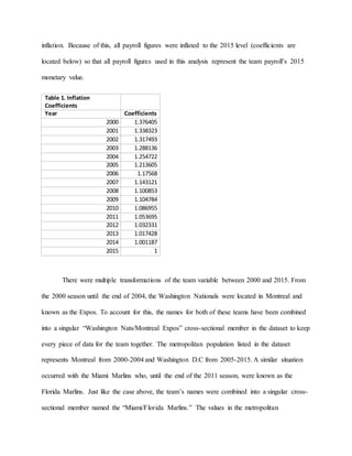
Alex Brakey
4/08/16
ECO 315-B
Professor Tebaldi
Does it really Pay to Play?
Section I. Introduction
All over television and the internet, you will see the astronomically high salaries that star
athletes make in professional sports. The professional sports league that is most famous for huge
contracts is Major League Baseball. The average team payroll on opening day in 2000 was over
$77 million (in 2015 dollars). On opening day 2015, the average payroll was $122 million
according to usatoday.com (2015). There are a few different theories about why payrolls have
increased so much in the past 15 years. One theory, hypothesized by Stephen Hall, Stefan
Szymanski, and Andrew Zimbalist (2002), is that players on winning teams have experienced
expectancy theory and require higher yearly salaries to maintain their level of play. Another
theory is that there is a link between a team’s performance and their payroll. This is the theory
which I will be testing in this paper.
This topic is important because it will answer the question that has been posed in bars and
on sports shows across America for years which is whether or not these large payrolls are based
on performance or if there are other factors that influence payroll. Does it make sense that the
2015 New York Yankees won 87 games while hitting .251, had a team ERA of 4.03, and had a
payroll north of $197 million while the 2015 Pittsburgh Pirates won 98 games while hitting .260,
had a team ERA of 3.21, and a payroll of just $86 million? I have chosen to research this topic
because I am one of those sports fans that is genuinely curious about whether my team’s payroll
is linked to performance or if the ever-rising payroll is just the result of capitalism in its finest
form.
The information and data that I will be referencing throughout this paper will come from
various scholarly articles that have been found using economics databases and Google scholar. I
have identified multiple sources which will be helpful in answering my research question. Using
these sources, I will attempt to create a model that provides an accurate depiction of what
different factors have an effect on a team’s payroll.
Section II of this paper provides academic sources which explain the theories that support
my model. Section III provides a description of the data used for the analysis, including
descriptive statistics and graphical representations of different variables. Section IV contains the
final models used and the results of the analysis, as well as an in-depth discussion about the
forms of the model and interpretations of the models. Section V will answer the question “Does
the empirical work done provide support for the theory?” This section will also contain a
summary of the results and a reflection on the work that has been carried out.
Section II. Theories behind the Model
Yu-Li Tao, Hwei-Lin Chuang, and Eric Lin’s research (2015) has provided a lot of
insight for me. Their study, called “Compensation and Performance in Major League Baseball:
Evidence from salary dispersion and team performance,” focused on the relationship between
compensation and performance in Major League Baseball between 1985 and 2013 (2015). One
thing that makes the analysis done by Tao, Chuang, and Lin different from my analysis is that
they were measuring the effects of individual players on team performance while using two
different payroll variables, payroll level and payroll’s relative position (2015). The variable that I
found most interesting was the market variable which accounted for each team’s market area.
The rationale they discussed was that a larger market leads to higher team revenues which turns
into higher payroll and would then allow a team to go out and get better players which is likely
to increase the team’s production (2015). In both the Bloom and GMM estimates, the market
variable was insignificant even at the .10 significance level (2015). While Tao, Chuang, and
Lin’s results showed that the market variable was insignificant, I believe that it is something that
is important to control for because of the fact that bigger markets, such as New York and San
Francisco, will normally have higher payrolls than smaller market teams, such as the Kansas City
Royals.
Mikhail Averbukh, Scott Brown, and Brian Chase’s research (2015) is more closely
related to what I am attempting to prove using my model, although there are some notable
differences. The main difference is that this study was done to determine an individual player’s
salary. Different models were created for two positions: pitchers and batters. Their research
measured multiple statistics for both positions (ERA, Wins, Losses, and Strikeouts for Pitchers
and Hits, Homeruns, Batting Average, Runs Batted In, and On Base Percentage). The data that
they used was based on the 2000 through the 2007 season. In creating fitted line plots, the “Pay
and Performance” study found a relatively strong, positive correlation between wins and salary.
The correlation coefficient between the two variables was .657 (2015). There was also a
relatively strong positive correlation between strikeouts (for pitchers) and salary in their model
(2015).
Stephen Hall, Stefan Szymanski, and Andrew Zimbalist’s research paper titled “Testing
Causality between Team Performance and Payroll” (2002) didn’t contribute any variables to my
model however some important theories were discussed as to why salaries have been increasing.
Hall, Szymanski, and Zimbalist stated that one of the main reasons of higher salaries is weak
free-agent classes during the offseason. The less free-agents available for a team, the more
willing a team will be to spend more on free-agents (2002). There is also the idea that players on
winning teams tend to establish an expectancy theory with regard to wage. The more the team
wins and the better the player performs, the higher the wage that player will expect to get from
the team they currently play for (2002).
David Hoaglin and Paul Velleman, in their analysis titled “A Critical Look at some of the
Analyses of Major League Baseball Salaries” (1995), reviewed the most common methods of
working with a team’s salary that were used by 15 different groups as part of a data analysis
exposition. What they found was that the salary variable was skewed and that most of the
possible predictors, when graphed against salary, were not linearly related (1995). The reasons
for re-expressing the salary variable in log form included making the distribution more
symmetric (the graph for inflation adjusted payroll and log of inflation adjusted payroll in
section III of this paper shows this), obtaining a better fit, stabilizing salary variance, and
accounting for year-by-year increases and decreases in bonus salaries. Hoaglin and Velleman
also found that those who worked with the re-expression of salary in log form were more
successful in creating an accurate model (1995).
Section III. The Data
The data that I will be using comes from all 30 MLB teams from the 2000 season to the
2015 season. Because this data contains a time series (2000-2015) for each cross-sectional
member (each MLB team), I am working with panel/longitudinal data. Team payroll information
was obtained from usatoday.com and provides the dollar figure for each team’s payroll for each
year. One important thing to note is that $1 in 2000 was not worth the same in 2015 due to
inflation. Because of this, all payroll figures were inflated to the 2015 level (coefficients are
located below) so that all payroll figures used in this analysis represent the team payroll’s 2015
monetary value.
Table 1. Inflation
Coefficients
Year Coefficients
2000 1.376405
2001 1.338323
2002 1.317493
2003 1.288136
2004 1.254722
2005 1.213605
2006 1.17568
2007 1.143121
2008 1.100853
2009 1.104784
2010 1.086955
2011 1.053695
2012 1.032331
2013 1.017428
2014 1.001187
2015 1
There were multiple transformations of the team variable between 2000 and 2015. From
the 2000 season until the end of 2004, the Washington Nationals were located in Montreal and
known as the Expos. To account for this, the names for both of these teams have been combined
into a singular “Washington Nats/Montreal Expos” cross-sectional member in the dataset to keep
every piece of data for the team together. The metropolitan population listed in the dataset
represents Montreal from 2000-2004 and Washington D.C from 2005-2015. A similar situation
occurred with the Miami Marlins who, until the end of the 2011 season, were known as the
Florida Marlins. Just like the case above, the team’s names were combined into a singular cross-
sectional member named the “Miami/Florida Marlins.” The values in the metropolitan
population variable are all from the greater Miami metropolitan area because the team was
located in that metropolitan area both before and after they moved.
The strength of the data being used is that it is not a sample of teams, it is all 30 MLB
teams over a 16 season period and, thus, a collection of data from the whole population of MLB
over those 16 seasons. This is a strength because all of the figures that are obtained in my
analysis will be representative of the entire population of MLB teams instead of just a fraction of
the teams. The one weakness with this data is that it is possible that heteroskedasticity is present.
This will have no effect on the slope of each variable however there will be an effect on the
variance in the standard errors which makes any t-test, f-test, or confidence intervals calculated
using normal estimators invalid. Because I have panel data, I cannot conduct the Breusch-Pagan
test or White test for heteroskedasticity. In order to account for possible heteroskedasticity, I will
work with the robust estimators for which ever model I end up using after conducting a Hausman
test.
Table 2. Descriptive Statistics
Variables: Mean St.
Deviation
Min Max
Log of Inf Adj Payroll 18.2911 0.427 16.685 19.348
Wins 80.97 11.42 43 116
RunsOffensive 739.54 84.82 513 978
HomerunsOffensive 166.67 33.56 91 260
SluggingPercentage 0.4144 0.02687 0.335 0.491
BattingPercentage 0.261 0.012 0.226 0.294
ERA 4.236 0.536 2.94 5.71
Log of PitcherStrikeouts 7.01 0.113 6.64 7.28
Log of PitcherWalks 6.25 0.129 5.85 6.59
FieldingPercentage 0.983 0.0027 0.976 0.991
Log of Metro.Population 15.052 0.589 14.22 16.48
SectionIV. Empirical Model and Results
Section IV. Part 1: Creating the Models
The following model will be estimated:
Log of inflation adj. payroll= 𝛽0 + 𝛽1( 𝑤𝑖𝑛𝑠) + 𝛽2( 𝑟𝑢𝑛𝑠 𝑜𝑓𝑓𝑒𝑛𝑠𝑖𝑣𝑒) +
𝛽3(ℎ𝑜𝑚𝑒𝑟𝑢𝑛𝑠 𝑜𝑓𝑓)+ 𝛽4( 𝑠𝑙𝑔 𝑝𝑒𝑟𝑐𝑒𝑛𝑡𝑎𝑔𝑒) + 𝛽5( 𝑏𝑎𝑡𝑡𝑖𝑛𝑔 𝑝𝑒𝑟𝑐𝑒𝑛𝑡𝑎𝑔𝑒) + 𝛽6( 𝑒𝑟𝑎) +
𝛽7(log 𝑝𝑖𝑡𝑐ℎ𝑒𝑟 𝑠𝑡𝑟𝑖𝑘𝑒𝑜𝑢𝑡𝑠) + 𝛽8(log 𝑝𝑖𝑡𝑐ℎ𝑒𝑟 𝑤𝑎𝑙𝑘𝑠) + 𝛽9( 𝑓𝑖𝑒𝑙𝑑𝑖𝑛𝑔 𝑝𝑒𝑟𝑐𝑒𝑛𝑡𝑎𝑔𝑒) +
𝛽10(log 𝑜𝑓 𝑚𝑒𝑡. 𝑝𝑜𝑝𝑢𝑙𝑎𝑡𝑖𝑜𝑛)
Deciding on the functional form of the variables was something that took some time to
figure out. One of the issues that I encountered was that my model contains some values that
represent an average (ex. Batting percentage, slugging percentage, and fielding percentage)
while others represent a certain numerical statistic which will be much greater than 1. I ran the
model originally with logs on just the inflation adjusted payroll and metropolitan population
because those numbers were in the millions and would have adversely effected my results. I
decided to put a log on inflation adjusted payroll, pitcher strikeouts, pitcher walks, and
metropolitan population because these numbers for each team tended to be relatively large. I did
not see the necessity of quadratics for any of the variables in my model.
Distribution of Metropolitan Population:
12500000100000007500000500000025000000-2500000
100
80
60
40
20
0
Mean 4187263
StDev 3017073
N 480
metpop
Frequency
Histogram of metpop
Normal
Distribution of Log of Metropolitan Population:
Taking the log of metropolitan population leads to a more normal distribution. It is more
likely that log of metropolitan population would pass the normality assumption when compared
to metropolitan population although log of metro population still isn’t very normally distributed.
It is necessary to use the log of metro population because this will rescale the values for each
cross-sectional member to a number which is closer to the scales of the other variables in the
dataset.
Distribution of Inflation Adjusted Payroll:
16.416.015.615.214.814.414.0
60
50
40
30
20
10
0
Mean 15.05
StDev 0.5895
N 480
lnmetpop
Frequency
Histogram of lnmetpop
Normal
240000000210000000180000000150000000120000000900000006000000030000000
70
60
50
40
30
20
10
0
Inf. Adj Payroll
Frequency
Histogram of Inf. Adj Payroll
Distribution of Log of Inflation Adjusted Payroll:
Both the inflation adjusted payroll and log of inflation adjusted payroll are relatively
normally distributed and both would likely pass the normality assumption, however the log of
inflation adjusted payroll variable is more normally distributed. As Hoaglin and Velleman
(1995) noted, a team’s salary tends to be skewed when it is in its standard form but then re-
expressing salary with a log will make the distributions more symmetric. Using log of inflation
adjusted payroll is necessary for this model because of the values of payroll for each team. With
each data point being in the millions, these points needed to be rescaled so that they were closer
to the values of the other variables in the dataset.
Upon determining which variables, and in what form, would be included in the model,
three models were predicted. The first was a simple ordinary least squares model. The OLS
regression model acts as more of a benchmark than a model that will actually be considered. The
OLS results (listed in Column 1 of Table 3 below) aren’t particularly interesting in solving the
question I posed earlier. This is because OLS models, when dealing with panel data, suffer from
omitted variable bias. We have not accounted for unobserved heterogeneity in OLS which means
that we know, for sure, that our estimates are wrong. We must move on and test two other
models in order to get an accurate answer for my research question.
19.218.818.418.017.617.216.8
60
50
40
30
20
10
0
lninfadjpayroll
Frequency
Histogram of lninfadjpayroll
Table 3. Model Results:
(OLS) (FE) (RE)
Log of Inf. Adj
Payroll
Log of Inf. Adj
Payroll
Log of Inf. Adj
Payroll
Wins 0.00371 0.00100 0.00274
(0.91) (0.31) (0.85)
Runs (Off) -0.000612 -0.000546 -0.000575
(-0.98) (-1.08) (-1.11)
Homeruns
(Off)
0.00747*** 0.00374* 0.00438**
(4.05) (2.29) (2.67)
Slugging Pct. -11.98*** -7.148* -8.252**
(-3.42) (-2.31) (-2.66)
Batting Pct. 24.42*** 12.30** 15.00***
(5.53) (3.19) (3.88)
ERA 0.0393 0.0628 0.0776
(0.48) (0.96) (1.17)
Log of
pitcher
strikeouts
0.872*** 0.828*** 0.770***
(4.60) (5.13) (4.77)
Log of
pitcher walks
-0.485** -0.561*** -0.520***
(-3.09) (-4.01) (-3.73)
Fielding Pct. 14.24* 13.23* 11.12*
(2.10) (2.41) (2.02)
Log of the
Metro. Pop
0.190*** -0.437 0.166**
(6.52) (-1.93) (2.62)
_cons -4.326 8.743 1.353
(-0.64) (1.47) (0.24)
N 480 480 480
t statistics in parentheses
* p < 0.05, ** p < 0.01, *** p < 0.001
The second model I ran was a fixed effects model (Listed in Column 2 of Table 3). Fixed
effects estimators are more consistent because, as the sample size increases, 𝛽̂ will get closer to
the true 𝛽. One thing that was interesting was the p-value and sign of the log of the metropolitan
population variable. The p-value of .054 indicates that it is statistically significant at a .10
significance level. This variable can be interpreted as meaning that every additional 1% increase
in the population of the team’s metropolitan area will decrease the team’s inflation adjusted
payroll by .437%, ceteris paribus. This is the opposite of what Tao, Chuang, and Lin (2015)
hypothesized in their analysis. When they ran their models, the market variable was not
significant at the .10 level (2015). In general, this model is saying that a larger metropolitan area
will actually decrease the teams inflation adjusted payroll. Another interesting result from the
fixed effects model was the slope and p-value for era. The slope and p-value were .0628 and
.337, respectively. The interesting point about this is that there is a positive relationship between
era and log of inflation adjusted payroll. In their pitchers equation, Averbukh, Brown, and Chase
(2015) found a negative correlation between era and salary which means that as era increases,
the salary of the team will decrease.
The third and final model that was estimated was a random effects model (Listed in
Column 3 of Table 3). Random effects estimators are more efficient because the estimators
provide smaller variance regressions, meaning the standard error for each coefficient will be
smallest in the random effects model. The coefficient for batting percentage had a p-value of
.000 which indicates that it is a very significant aspect when looking at a team’s inflation
adjusted payroll. This coefficient indicates that for each additional 1% increase in batting
percentage, the teams inflation adjusted payroll will increase by 15%, ceteris paribus. Another
variable that was significant in the random effects model was log of the pitcher walks. For each
additional 1% increase in walks by the pitching staff, inflation adjusted payroll will decrease by
about .52%, ceteris paribus. When comparing the random and fixed effects models, we can also
see that the p-values for wins and runs (off) decreased when going from the fixed effects
estimates to the random effects estimates.
To determine which model should be used, a Hausman test was conducted and a
significance level of .05 for rejection was set. The null hypothesis was that the random effects
model was better. The alternative hypothesis was that the fixed effects model was better. The test
resulted in a chi-square value of 16.04 and a p-value of .0661. With a p-value above our .05
significance level, we fail to reject the null hypothesis which means that we are 95% confident
that the random effects model is the best model to use for this analysis. As mentioned above,
while we know that we are using the right model after conducting the Hausman test, it is still
possible that our estimators are inaccurate due to heteroskedasticity. In order to account for this,
we need to look at the robust estimators of the random effects model. We will notice that the
coefficient itself will not change, but everything else will. One of the consequences of
heteroskedasticity is that the variance in the standard errors incorrect which will make any t-test,
f-test, or confidence interval invalid using those incorrect standard errors. This would make any
tests for significance inaccurate. Using the robust estimators is a way for us to correct for
heteroskedasticity and make all of our standard error estimates correct.
Section VI. Part 3: Interpreting the RE Model with Robust Estimators
The overall 𝑅2
of the model is .2997 which means that 29.97% of the total variation in log
of inflation adjusted payroll can be explained over time and across cross-sectional units using this
model. The between 𝑅2
is .4110 which means that 41.1% of the total variation in log of inflation
adjusted payroll between cross-sectional units can be explained using this model.
Table 4. Robust Estimators of the Random Effects Model:
(RE Robust)
Log of Inf. Adj
Payroll
Wins 0.00274
(0.91)
Runs (Off) -0.000575
(-1.20)
Homeruns
(Off)
0.00438*
(2.33)
Slugging Pct. -8.252*
(-2.22)
Off. Bat
Proportion
15.00***
(3.71)
ERA 0.0776
(1.09)
Log of pitcher
strikeouts
0.770***
(4.49)
Log of pitcher
walks
-0.520***
(-3.67)
Fielding Pct. 11.12*
(2.01)
Log of the
Metro Pop
0.166**
(2.62)
_cons 1.353
(0.25)
N 480
t statistics in parentheses
* p < 0.05, ** p < 0.01, *** p < 0.001
Standard errors are calculated using robust estimators
Both home runs (off) and slugging percentage were significant at the .01 level in the model
without robust errors. Both of these variables became less significant, though still significant at
the .05 level, when we calculated the robust estimators. The interpretation of home runs (off) is
that for each additional homerun a team hits, the team’s inflation adjusted payroll will increase by
.438%, ceteris paribus. In this model, slugging percentage is significant at the .05 level. The
variables coefficient means that for each additional 1% increase in slugging percentage, a team’s
inflation adjusted payroll will decrease by 8.25%, ceteris paribus. The variable log of the
metropolitan population is significant at the .01 level. In Tao, Chuang, and Lin’s analysis (2015),
their Market variable was insignificant at even the .10 level. The relationship between log of the
metropolitan population and log of inflation adjusted payroll is what we would expect. For every
1% increase in metropolitan population, inflation adjusted payroll will increase by .166%, ceteris
paribus. This supports the theory presented in Tao, Chuang, and Lin’s analysis (2015) that a higher
market population will allow for teams to increase payrolls and get better players.
Section V. Conclusion
The theory that was being tested in this analysis was that there was a link between a
team’s performance and their payroll. Upon finding which model would be the best to use for
this analysis, we can conclude that there is a link between the team’s performance and their
payroll, though other factors definitely play a role in determining a team’s payroll. So, to answer
the question posed in Section I, the empirical work done does provide some support for the
theory but there are other factors that should be controlled for to get the most accurate answer.
We know that there are other factors in play because of the between and overall 𝑅2
values. Apart
from the key performance indicators that were controlled for in the model, nearly 60% of the
variation in log of inflation adjusted payroll between cross-sectional units remains unexplained.
Almost every key performance variable included in this analysis was significant at the .05
level which indicates that these variables did have an effect on a team’s payroll. The log of
metropolitan population variable makes me hesitant to say that performance is the only
determinant of a team’s payroll. In Averbukh, Chase, and Brown’s analysis (2015), they
concluded that performance is only generally linked to pay and that there are definitely outside
factors that affect payrolls. Tao, Chuang, and Lin (2015) also found that there is a link between
performance and payroll. I believe that my conclusion aligns with what Averbukh, Chase, and
Brown (2015) found which is that there is only a general link between salary and performance in
Major League Baseball.
I believe that I could have accomplished quite a bit more with this project. The only issue
with everything that I wanted to do was time. One variable was age. I was going to find the
average age for each team for each year and then I was going to include both a linear age
variable and a quadratic age variable. “Pay, Productivity, and Aging in Major League Baseball”
(2011) authors Jahn Hakes and Chad Turner suggested that the age variable follows a quadratic
pattern. Up until the age 27, a player’s age has a positive return to performance. After 27 though,
a player’s performance will begin to decline (2011). I believe that including age, in both linear
and quadratic form, would have benefited my model because it would have accounted for what
Hakes and Turner were able to show which is that age is significant to both performance and
salary. Another variable that I would have added given more time would be Gini coefficients.
The Gini coefficient measures the inequality among values of a frequency distribution and is
commonly used to measure income inequality.
Work Cited
Averbukh, M., Brown, S., & Chase, B. (2015). Baseball Pay and Performance (PDF) [PDF].
Retrieved March 09, 2016, from https://ai.arizona.edu/sites/ai/files/MIS580/baseball.pdf
Hakes, J. K., & Turner, C. (2011). Pay, productivity and aging in Major League
Baseball. Journal of Productivity Analysis, 35(1), 61-74.
Hall, S., Szymanski, S., & Zimablist, A. (2002). Testing Causality between Team Performance
and Payroll. Journal of Sports Economics. Retrieved April 12, 2016, from
http://jse.sagepub.com/content/3/2/149.full.pdf html
Hoaglin, David C., and Paul F. Velleman. "A critical look at some analyses of major league
baseball salaries." The American Statistician 49.3 (1995): 277-285.
Tao, Y. L., Chuang, H. L., & Lin, E. S. (2015). Compensation and performance in Major League
Baseball: Evidence from salary dispersion and team performance. International Review
of Economics & Finance.
United States, U.S Census Bureau. (2010). Population Change for Metropolitan and
Micropolitan Statistical Areas in the United States and Puerto Rico: 2000 to 2010 (CPH-
T-2). DC.
United States, U.S Census Bureau. (2015). Annual Estimates of the Resident Population: April 1,
2010 to July 1, 2015 - United States – Metropolitan and Micropolitan Statistical Area;
and for Puerto Rico: 2015 Population Estimates. DC.
Data information:
For Payroll information: http://www.usatoday.com/sports/mlb/salaries/2000/team/all/
For Team statistics:
http://mlb.mlb.com/stats/sortable.jsp#elem=%5Bobject+Object%5D&tab_level=child&cl
ick_text=Sortable+Team+hitting&game_type='R'&season=2015&season_type=ANY&le
ague_code='MLB'&sectionType=st&statType=hitting&page=1&ts=1462233385078&pla
yerType=ALL&sportCode='mlb'&split=&team_id=&active_sw=&position=&page_type
=SortablePlayer&sortOrder='desc'&sortColumn=avg&results=&perPage=50&timeframe
=&last_x_days=&extended=0

Econometrics Paper

  • 1.
    Alex Brakey 4/08/16 ECO 315-B ProfessorTebaldi Does it really Pay to Play? Section I. Introduction All over television and the internet, you will see the astronomically high salaries that star athletes make in professional sports. The professional sports league that is most famous for huge contracts is Major League Baseball. The average team payroll on opening day in 2000 was over $77 million (in 2015 dollars). On opening day 2015, the average payroll was $122 million according to usatoday.com (2015). There are a few different theories about why payrolls have increased so much in the past 15 years. One theory, hypothesized by Stephen Hall, Stefan Szymanski, and Andrew Zimbalist (2002), is that players on winning teams have experienced expectancy theory and require higher yearly salaries to maintain their level of play. Another theory is that there is a link between a team’s performance and their payroll. This is the theory which I will be testing in this paper. This topic is important because it will answer the question that has been posed in bars and on sports shows across America for years which is whether or not these large payrolls are based on performance or if there are other factors that influence payroll. Does it make sense that the 2015 New York Yankees won 87 games while hitting .251, had a team ERA of 4.03, and had a payroll north of $197 million while the 2015 Pittsburgh Pirates won 98 games while hitting .260, had a team ERA of 3.21, and a payroll of just $86 million? I have chosen to research this topic because I am one of those sports fans that is genuinely curious about whether my team’s payroll
  • 2.
    is linked toperformance or if the ever-rising payroll is just the result of capitalism in its finest form. The information and data that I will be referencing throughout this paper will come from various scholarly articles that have been found using economics databases and Google scholar. I have identified multiple sources which will be helpful in answering my research question. Using these sources, I will attempt to create a model that provides an accurate depiction of what different factors have an effect on a team’s payroll. Section II of this paper provides academic sources which explain the theories that support my model. Section III provides a description of the data used for the analysis, including descriptive statistics and graphical representations of different variables. Section IV contains the final models used and the results of the analysis, as well as an in-depth discussion about the forms of the model and interpretations of the models. Section V will answer the question “Does the empirical work done provide support for the theory?” This section will also contain a summary of the results and a reflection on the work that has been carried out. Section II. Theories behind the Model Yu-Li Tao, Hwei-Lin Chuang, and Eric Lin’s research (2015) has provided a lot of insight for me. Their study, called “Compensation and Performance in Major League Baseball: Evidence from salary dispersion and team performance,” focused on the relationship between compensation and performance in Major League Baseball between 1985 and 2013 (2015). One thing that makes the analysis done by Tao, Chuang, and Lin different from my analysis is that they were measuring the effects of individual players on team performance while using two different payroll variables, payroll level and payroll’s relative position (2015). The variable that I
  • 3.
    found most interestingwas the market variable which accounted for each team’s market area. The rationale they discussed was that a larger market leads to higher team revenues which turns into higher payroll and would then allow a team to go out and get better players which is likely to increase the team’s production (2015). In both the Bloom and GMM estimates, the market variable was insignificant even at the .10 significance level (2015). While Tao, Chuang, and Lin’s results showed that the market variable was insignificant, I believe that it is something that is important to control for because of the fact that bigger markets, such as New York and San Francisco, will normally have higher payrolls than smaller market teams, such as the Kansas City Royals. Mikhail Averbukh, Scott Brown, and Brian Chase’s research (2015) is more closely related to what I am attempting to prove using my model, although there are some notable differences. The main difference is that this study was done to determine an individual player’s salary. Different models were created for two positions: pitchers and batters. Their research measured multiple statistics for both positions (ERA, Wins, Losses, and Strikeouts for Pitchers and Hits, Homeruns, Batting Average, Runs Batted In, and On Base Percentage). The data that they used was based on the 2000 through the 2007 season. In creating fitted line plots, the “Pay and Performance” study found a relatively strong, positive correlation between wins and salary. The correlation coefficient between the two variables was .657 (2015). There was also a relatively strong positive correlation between strikeouts (for pitchers) and salary in their model (2015). Stephen Hall, Stefan Szymanski, and Andrew Zimbalist’s research paper titled “Testing Causality between Team Performance and Payroll” (2002) didn’t contribute any variables to my model however some important theories were discussed as to why salaries have been increasing.
  • 4.
    Hall, Szymanski, andZimbalist stated that one of the main reasons of higher salaries is weak free-agent classes during the offseason. The less free-agents available for a team, the more willing a team will be to spend more on free-agents (2002). There is also the idea that players on winning teams tend to establish an expectancy theory with regard to wage. The more the team wins and the better the player performs, the higher the wage that player will expect to get from the team they currently play for (2002). David Hoaglin and Paul Velleman, in their analysis titled “A Critical Look at some of the Analyses of Major League Baseball Salaries” (1995), reviewed the most common methods of working with a team’s salary that were used by 15 different groups as part of a data analysis exposition. What they found was that the salary variable was skewed and that most of the possible predictors, when graphed against salary, were not linearly related (1995). The reasons for re-expressing the salary variable in log form included making the distribution more symmetric (the graph for inflation adjusted payroll and log of inflation adjusted payroll in section III of this paper shows this), obtaining a better fit, stabilizing salary variance, and accounting for year-by-year increases and decreases in bonus salaries. Hoaglin and Velleman also found that those who worked with the re-expression of salary in log form were more successful in creating an accurate model (1995). Section III. The Data The data that I will be using comes from all 30 MLB teams from the 2000 season to the 2015 season. Because this data contains a time series (2000-2015) for each cross-sectional member (each MLB team), I am working with panel/longitudinal data. Team payroll information was obtained from usatoday.com and provides the dollar figure for each team’s payroll for each year. One important thing to note is that $1 in 2000 was not worth the same in 2015 due to
  • 5.
    inflation. Because ofthis, all payroll figures were inflated to the 2015 level (coefficients are located below) so that all payroll figures used in this analysis represent the team payroll’s 2015 monetary value. Table 1. Inflation Coefficients Year Coefficients 2000 1.376405 2001 1.338323 2002 1.317493 2003 1.288136 2004 1.254722 2005 1.213605 2006 1.17568 2007 1.143121 2008 1.100853 2009 1.104784 2010 1.086955 2011 1.053695 2012 1.032331 2013 1.017428 2014 1.001187 2015 1 There were multiple transformations of the team variable between 2000 and 2015. From the 2000 season until the end of 2004, the Washington Nationals were located in Montreal and known as the Expos. To account for this, the names for both of these teams have been combined into a singular “Washington Nats/Montreal Expos” cross-sectional member in the dataset to keep every piece of data for the team together. The metropolitan population listed in the dataset represents Montreal from 2000-2004 and Washington D.C from 2005-2015. A similar situation occurred with the Miami Marlins who, until the end of the 2011 season, were known as the Florida Marlins. Just like the case above, the team’s names were combined into a singular cross- sectional member named the “Miami/Florida Marlins.” The values in the metropolitan
  • 6.
    population variable areall from the greater Miami metropolitan area because the team was located in that metropolitan area both before and after they moved. The strength of the data being used is that it is not a sample of teams, it is all 30 MLB teams over a 16 season period and, thus, a collection of data from the whole population of MLB over those 16 seasons. This is a strength because all of the figures that are obtained in my analysis will be representative of the entire population of MLB teams instead of just a fraction of the teams. The one weakness with this data is that it is possible that heteroskedasticity is present. This will have no effect on the slope of each variable however there will be an effect on the variance in the standard errors which makes any t-test, f-test, or confidence intervals calculated using normal estimators invalid. Because I have panel data, I cannot conduct the Breusch-Pagan test or White test for heteroskedasticity. In order to account for possible heteroskedasticity, I will work with the robust estimators for which ever model I end up using after conducting a Hausman test. Table 2. Descriptive Statistics Variables: Mean St. Deviation Min Max Log of Inf Adj Payroll 18.2911 0.427 16.685 19.348 Wins 80.97 11.42 43 116 RunsOffensive 739.54 84.82 513 978 HomerunsOffensive 166.67 33.56 91 260 SluggingPercentage 0.4144 0.02687 0.335 0.491 BattingPercentage 0.261 0.012 0.226 0.294 ERA 4.236 0.536 2.94 5.71 Log of PitcherStrikeouts 7.01 0.113 6.64 7.28 Log of PitcherWalks 6.25 0.129 5.85 6.59 FieldingPercentage 0.983 0.0027 0.976 0.991 Log of Metro.Population 15.052 0.589 14.22 16.48
  • 7.
    SectionIV. Empirical Modeland Results Section IV. Part 1: Creating the Models The following model will be estimated: Log of inflation adj. payroll= 𝛽0 + 𝛽1( 𝑤𝑖𝑛𝑠) + 𝛽2( 𝑟𝑢𝑛𝑠 𝑜𝑓𝑓𝑒𝑛𝑠𝑖𝑣𝑒) + 𝛽3(ℎ𝑜𝑚𝑒𝑟𝑢𝑛𝑠 𝑜𝑓𝑓)+ 𝛽4( 𝑠𝑙𝑔 𝑝𝑒𝑟𝑐𝑒𝑛𝑡𝑎𝑔𝑒) + 𝛽5( 𝑏𝑎𝑡𝑡𝑖𝑛𝑔 𝑝𝑒𝑟𝑐𝑒𝑛𝑡𝑎𝑔𝑒) + 𝛽6( 𝑒𝑟𝑎) + 𝛽7(log 𝑝𝑖𝑡𝑐ℎ𝑒𝑟 𝑠𝑡𝑟𝑖𝑘𝑒𝑜𝑢𝑡𝑠) + 𝛽8(log 𝑝𝑖𝑡𝑐ℎ𝑒𝑟 𝑤𝑎𝑙𝑘𝑠) + 𝛽9( 𝑓𝑖𝑒𝑙𝑑𝑖𝑛𝑔 𝑝𝑒𝑟𝑐𝑒𝑛𝑡𝑎𝑔𝑒) + 𝛽10(log 𝑜𝑓 𝑚𝑒𝑡. 𝑝𝑜𝑝𝑢𝑙𝑎𝑡𝑖𝑜𝑛) Deciding on the functional form of the variables was something that took some time to figure out. One of the issues that I encountered was that my model contains some values that represent an average (ex. Batting percentage, slugging percentage, and fielding percentage) while others represent a certain numerical statistic which will be much greater than 1. I ran the model originally with logs on just the inflation adjusted payroll and metropolitan population because those numbers were in the millions and would have adversely effected my results. I decided to put a log on inflation adjusted payroll, pitcher strikeouts, pitcher walks, and metropolitan population because these numbers for each team tended to be relatively large. I did not see the necessity of quadratics for any of the variables in my model. Distribution of Metropolitan Population: 12500000100000007500000500000025000000-2500000 100 80 60 40 20 0 Mean 4187263 StDev 3017073 N 480 metpop Frequency Histogram of metpop Normal
  • 8.
    Distribution of Logof Metropolitan Population: Taking the log of metropolitan population leads to a more normal distribution. It is more likely that log of metropolitan population would pass the normality assumption when compared to metropolitan population although log of metro population still isn’t very normally distributed. It is necessary to use the log of metro population because this will rescale the values for each cross-sectional member to a number which is closer to the scales of the other variables in the dataset. Distribution of Inflation Adjusted Payroll: 16.416.015.615.214.814.414.0 60 50 40 30 20 10 0 Mean 15.05 StDev 0.5895 N 480 lnmetpop Frequency Histogram of lnmetpop Normal 240000000210000000180000000150000000120000000900000006000000030000000 70 60 50 40 30 20 10 0 Inf. Adj Payroll Frequency Histogram of Inf. Adj Payroll
  • 9.
    Distribution of Logof Inflation Adjusted Payroll: Both the inflation adjusted payroll and log of inflation adjusted payroll are relatively normally distributed and both would likely pass the normality assumption, however the log of inflation adjusted payroll variable is more normally distributed. As Hoaglin and Velleman (1995) noted, a team’s salary tends to be skewed when it is in its standard form but then re- expressing salary with a log will make the distributions more symmetric. Using log of inflation adjusted payroll is necessary for this model because of the values of payroll for each team. With each data point being in the millions, these points needed to be rescaled so that they were closer to the values of the other variables in the dataset. Upon determining which variables, and in what form, would be included in the model, three models were predicted. The first was a simple ordinary least squares model. The OLS regression model acts as more of a benchmark than a model that will actually be considered. The OLS results (listed in Column 1 of Table 3 below) aren’t particularly interesting in solving the question I posed earlier. This is because OLS models, when dealing with panel data, suffer from omitted variable bias. We have not accounted for unobserved heterogeneity in OLS which means that we know, for sure, that our estimates are wrong. We must move on and test two other models in order to get an accurate answer for my research question. 19.218.818.418.017.617.216.8 60 50 40 30 20 10 0 lninfadjpayroll Frequency Histogram of lninfadjpayroll
  • 10.
    Table 3. ModelResults: (OLS) (FE) (RE) Log of Inf. Adj Payroll Log of Inf. Adj Payroll Log of Inf. Adj Payroll Wins 0.00371 0.00100 0.00274 (0.91) (0.31) (0.85) Runs (Off) -0.000612 -0.000546 -0.000575 (-0.98) (-1.08) (-1.11) Homeruns (Off) 0.00747*** 0.00374* 0.00438** (4.05) (2.29) (2.67) Slugging Pct. -11.98*** -7.148* -8.252** (-3.42) (-2.31) (-2.66) Batting Pct. 24.42*** 12.30** 15.00*** (5.53) (3.19) (3.88) ERA 0.0393 0.0628 0.0776 (0.48) (0.96) (1.17) Log of pitcher strikeouts 0.872*** 0.828*** 0.770*** (4.60) (5.13) (4.77) Log of pitcher walks -0.485** -0.561*** -0.520*** (-3.09) (-4.01) (-3.73) Fielding Pct. 14.24* 13.23* 11.12* (2.10) (2.41) (2.02) Log of the Metro. Pop 0.190*** -0.437 0.166** (6.52) (-1.93) (2.62) _cons -4.326 8.743 1.353 (-0.64) (1.47) (0.24) N 480 480 480 t statistics in parentheses * p < 0.05, ** p < 0.01, *** p < 0.001
  • 11.
    The second modelI ran was a fixed effects model (Listed in Column 2 of Table 3). Fixed effects estimators are more consistent because, as the sample size increases, 𝛽̂ will get closer to the true 𝛽. One thing that was interesting was the p-value and sign of the log of the metropolitan population variable. The p-value of .054 indicates that it is statistically significant at a .10 significance level. This variable can be interpreted as meaning that every additional 1% increase in the population of the team’s metropolitan area will decrease the team’s inflation adjusted payroll by .437%, ceteris paribus. This is the opposite of what Tao, Chuang, and Lin (2015) hypothesized in their analysis. When they ran their models, the market variable was not significant at the .10 level (2015). In general, this model is saying that a larger metropolitan area will actually decrease the teams inflation adjusted payroll. Another interesting result from the fixed effects model was the slope and p-value for era. The slope and p-value were .0628 and .337, respectively. The interesting point about this is that there is a positive relationship between era and log of inflation adjusted payroll. In their pitchers equation, Averbukh, Brown, and Chase (2015) found a negative correlation between era and salary which means that as era increases, the salary of the team will decrease. The third and final model that was estimated was a random effects model (Listed in Column 3 of Table 3). Random effects estimators are more efficient because the estimators provide smaller variance regressions, meaning the standard error for each coefficient will be smallest in the random effects model. The coefficient for batting percentage had a p-value of .000 which indicates that it is a very significant aspect when looking at a team’s inflation adjusted payroll. This coefficient indicates that for each additional 1% increase in batting percentage, the teams inflation adjusted payroll will increase by 15%, ceteris paribus. Another variable that was significant in the random effects model was log of the pitcher walks. For each
  • 12.
    additional 1% increasein walks by the pitching staff, inflation adjusted payroll will decrease by about .52%, ceteris paribus. When comparing the random and fixed effects models, we can also see that the p-values for wins and runs (off) decreased when going from the fixed effects estimates to the random effects estimates. To determine which model should be used, a Hausman test was conducted and a significance level of .05 for rejection was set. The null hypothesis was that the random effects model was better. The alternative hypothesis was that the fixed effects model was better. The test resulted in a chi-square value of 16.04 and a p-value of .0661. With a p-value above our .05 significance level, we fail to reject the null hypothesis which means that we are 95% confident that the random effects model is the best model to use for this analysis. As mentioned above, while we know that we are using the right model after conducting the Hausman test, it is still possible that our estimators are inaccurate due to heteroskedasticity. In order to account for this, we need to look at the robust estimators of the random effects model. We will notice that the coefficient itself will not change, but everything else will. One of the consequences of heteroskedasticity is that the variance in the standard errors incorrect which will make any t-test, f-test, or confidence interval invalid using those incorrect standard errors. This would make any tests for significance inaccurate. Using the robust estimators is a way for us to correct for heteroskedasticity and make all of our standard error estimates correct. Section VI. Part 3: Interpreting the RE Model with Robust Estimators The overall 𝑅2 of the model is .2997 which means that 29.97% of the total variation in log of inflation adjusted payroll can be explained over time and across cross-sectional units using this model. The between 𝑅2 is .4110 which means that 41.1% of the total variation in log of inflation adjusted payroll between cross-sectional units can be explained using this model.
  • 13.
    Table 4. RobustEstimators of the Random Effects Model: (RE Robust) Log of Inf. Adj Payroll Wins 0.00274 (0.91) Runs (Off) -0.000575 (-1.20) Homeruns (Off) 0.00438* (2.33) Slugging Pct. -8.252* (-2.22) Off. Bat Proportion 15.00*** (3.71) ERA 0.0776 (1.09) Log of pitcher strikeouts 0.770*** (4.49) Log of pitcher walks -0.520*** (-3.67) Fielding Pct. 11.12* (2.01) Log of the Metro Pop 0.166** (2.62) _cons 1.353 (0.25) N 480 t statistics in parentheses * p < 0.05, ** p < 0.01, *** p < 0.001 Standard errors are calculated using robust estimators
  • 14.
    Both home runs(off) and slugging percentage were significant at the .01 level in the model without robust errors. Both of these variables became less significant, though still significant at the .05 level, when we calculated the robust estimators. The interpretation of home runs (off) is that for each additional homerun a team hits, the team’s inflation adjusted payroll will increase by .438%, ceteris paribus. In this model, slugging percentage is significant at the .05 level. The variables coefficient means that for each additional 1% increase in slugging percentage, a team’s inflation adjusted payroll will decrease by 8.25%, ceteris paribus. The variable log of the metropolitan population is significant at the .01 level. In Tao, Chuang, and Lin’s analysis (2015), their Market variable was insignificant at even the .10 level. The relationship between log of the metropolitan population and log of inflation adjusted payroll is what we would expect. For every 1% increase in metropolitan population, inflation adjusted payroll will increase by .166%, ceteris paribus. This supports the theory presented in Tao, Chuang, and Lin’s analysis (2015) that a higher market population will allow for teams to increase payrolls and get better players. Section V. Conclusion The theory that was being tested in this analysis was that there was a link between a team’s performance and their payroll. Upon finding which model would be the best to use for this analysis, we can conclude that there is a link between the team’s performance and their payroll, though other factors definitely play a role in determining a team’s payroll. So, to answer the question posed in Section I, the empirical work done does provide some support for the theory but there are other factors that should be controlled for to get the most accurate answer. We know that there are other factors in play because of the between and overall 𝑅2 values. Apart from the key performance indicators that were controlled for in the model, nearly 60% of the
  • 15.
    variation in logof inflation adjusted payroll between cross-sectional units remains unexplained. Almost every key performance variable included in this analysis was significant at the .05 level which indicates that these variables did have an effect on a team’s payroll. The log of metropolitan population variable makes me hesitant to say that performance is the only determinant of a team’s payroll. In Averbukh, Chase, and Brown’s analysis (2015), they concluded that performance is only generally linked to pay and that there are definitely outside factors that affect payrolls. Tao, Chuang, and Lin (2015) also found that there is a link between performance and payroll. I believe that my conclusion aligns with what Averbukh, Chase, and Brown (2015) found which is that there is only a general link between salary and performance in Major League Baseball. I believe that I could have accomplished quite a bit more with this project. The only issue with everything that I wanted to do was time. One variable was age. I was going to find the average age for each team for each year and then I was going to include both a linear age variable and a quadratic age variable. “Pay, Productivity, and Aging in Major League Baseball” (2011) authors Jahn Hakes and Chad Turner suggested that the age variable follows a quadratic pattern. Up until the age 27, a player’s age has a positive return to performance. After 27 though, a player’s performance will begin to decline (2011). I believe that including age, in both linear and quadratic form, would have benefited my model because it would have accounted for what Hakes and Turner were able to show which is that age is significant to both performance and salary. Another variable that I would have added given more time would be Gini coefficients. The Gini coefficient measures the inequality among values of a frequency distribution and is commonly used to measure income inequality.
  • 16.
    Work Cited Averbukh, M.,Brown, S., & Chase, B. (2015). Baseball Pay and Performance (PDF) [PDF]. Retrieved March 09, 2016, from https://ai.arizona.edu/sites/ai/files/MIS580/baseball.pdf Hakes, J. K., & Turner, C. (2011). Pay, productivity and aging in Major League Baseball. Journal of Productivity Analysis, 35(1), 61-74. Hall, S., Szymanski, S., & Zimablist, A. (2002). Testing Causality between Team Performance and Payroll. Journal of Sports Economics. Retrieved April 12, 2016, from http://jse.sagepub.com/content/3/2/149.full.pdf html Hoaglin, David C., and Paul F. Velleman. "A critical look at some analyses of major league baseball salaries." The American Statistician 49.3 (1995): 277-285. Tao, Y. L., Chuang, H. L., & Lin, E. S. (2015). Compensation and performance in Major League Baseball: Evidence from salary dispersion and team performance. International Review of Economics & Finance. United States, U.S Census Bureau. (2010). Population Change for Metropolitan and Micropolitan Statistical Areas in the United States and Puerto Rico: 2000 to 2010 (CPH- T-2). DC. United States, U.S Census Bureau. (2015). Annual Estimates of the Resident Population: April 1, 2010 to July 1, 2015 - United States – Metropolitan and Micropolitan Statistical Area; and for Puerto Rico: 2015 Population Estimates. DC.
  • 17.
    Data information: For Payrollinformation: http://www.usatoday.com/sports/mlb/salaries/2000/team/all/ For Team statistics: http://mlb.mlb.com/stats/sortable.jsp#elem=%5Bobject+Object%5D&tab_level=child&cl ick_text=Sortable+Team+hitting&game_type='R'&season=2015&season_type=ANY&le ague_code='MLB'&sectionType=st&statType=hitting&page=1&ts=1462233385078&pla yerType=ALL&sportCode='mlb'&split=&team_id=&active_sw=&position=&page_type =SortablePlayer&sortOrder='desc'&sortColumn=avg&results=&perPage=50&timeframe =&last_x_days=&extended=0