The document contains a series of multiple choice questions related to statistical concepts like probability distributions, expected values, variances, hypothesis testing, and errors. It covers topics like determining values in probability distributions, calculating statistical properties of random variables, interpreting hypothesis tests and critical values, and understanding how sample size and type I/II errors relate to statistical power.

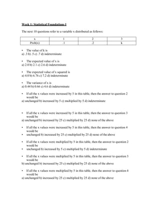
1. Week 1: Statistical Foundations I
The next 10 questions refer to a variable x distributed as follows:
x 1 2 3
Prob(x) .1 .2 k
• The value of k is
a) .3 b) .5 c) .7 d) indeterminate
• The expected value of x is
a) 2.0 b) 2.1 c) 2.6 d) indeterminate
• The expected value of x squared is
a) 4.0 b) 6.76 c) 7.2 d) indeterminate
• The variance of x is
a) 0.44 b) 0.66 c) 4.6 d) indeterminate
• If all the x values were increased by 5 in this table, then the answer to question 2
would be
a) unchanged b) increased by 5 c) multiplied by 5 d) indeterminate
• If all the x values were increased by 5 in this table, then the answer to question 3
would be
a) unchanged b) increased by 25 c) multiplied by 25 d) none of the above
• If all the x values were increased by 5 in this table, then the answer to question 4
would be
• unchanged b) increased by 25 c) multiplied by 25 d) none of the above
• If all the x values were multiplied by 5 in this table, then the answer to question 2
would be
• unchanged b) increased by 5 c) multiplied by 5 d) indeterminate
• If all the x values were multiplied by 5 in this table, then the answer to question 3
would be
b) unchanged b) increased by 25 c) multiplied by 25 d) none of the above
• If all the x values were multiplied by 5 in this table, then the answer to question 4
would be
a) unchanged b) increased by 25 c) multiplied by 25 d) none of the above

2. The next 17 questions refer to variables X and Y with the following joint distribution
prob(X,Y)
Y=4 Y=5 Y=6
X=1 .1 .05 k
X=2 .05 .1 .1
X=3 .1 .1 .4
• The value of k is
a) 0 b) .1 c) .2 d) indeterminate
• If I know that Y=4, then the probability that X=3 is a)
.1 b) .25 c) .4 d) .6
• If I don’t know anything about the value of Y, then the probability that X=3 is a)
.1 b) .2 c) .4 d) .6
• If I know that Y=5, then the expected value of X is a)
0.55 b) 2.0 c) 2.2 d) 2.5
• If I don’t know anything about Y, then the expected value of x is
a) 2.0 b) 2.25 c) 2.45 d) indeterminate
• If I know that Y=5, then the variance of X is a)
.56 b) .75 c) 4.84 d) 5.4
• If I don’t know anything about Y, then the variance of x is a)
.55 b) .74 c) 6.0 d) 6.55
• The covariance between X and Y is a)
0.0 b) .09 c) .19 d) .29
• The correlation between X and Y is a)
0.0 b) .29 c) .47 d) .54
• If all the X values in the table above were increased by 8, then the answer to question
18 would be
a) unchanged b) increased by 8 c) multiplied by 8 d) multiplied by 64
• If all the X values in the table above were increased by 8, then the answer to question
19 would be
a) unchanged b) increased by 8 c) multiplied by 8 d) multiplied by 64
• If all the X values and all the Y values in the table above were increased by 8, then
the answer to question 18 would be

3. a) unchanged b) increased by 8 c) multiplied by 8 d) multiplied by 64
• If all the X values and all the Y values in the table above were increased by 8, then
the answer to question 19 would be
a) unchanged b) increased by 8 c) multiplied by 8 d) multiplied by 64
• If all the X values in the table above were multiplied by 8, then the answer to question
18 would be
a) unchanged b) increased by 8 c) multiplied by 8 d) multiplied by 64
• If all the X values in the table above were multiplied by 8, then the answer to question
19 would be
a) unchanged b) increased by 8 c) multiplied by 8 d) multiplied by 64
• If all the X values and all the Y values in the table above were multiplied by 8, then
the answer to question 18 would be
a) unchanged b) increased by 8 c) multiplied by 8 d) multiplied by 64
• If all the X values and all the Y values in the table above were multiplied by 8, then
the answer to question 19 would be
a) unchanged b) increased by 8 c) multiplied by 8 d) multiplied by 64
• The distribution of X when Y is known is called the distribution of X, and is
written as . These blanks are best filled with
a) conditional, p(X) b) conditional, p(X Y)
c) marginal, p(X) d) marginal, p(X Y)
• The distribution of X when Y is not known iscalled the distribution of X,
and is written as . These blanks are best filled with
a) conditional, p(X) b) conditional, p(X Y)
c) marginal, p(X) d) marginal, p(X Y)
The next 5 questions refer to the following information. You have estimated the equation
wage = alphahat + betahat*experience to predict a person’s wage using years of experience
as an explanatory variable. Your results are that alphahat is 5.0 with standard error 0.8,
betahat is 1.2 with standard error 0.1, and the estimated covariance between alphahat and
betahat is –0.005. What this means is that 5.0 is a realization of a random variable with
unknown mean and standard error 1.0, and 1.2 is a realization of another random variable
which has unknown mean and standard error 0.01.
• The estimated variance of your forecast of the wage of a person with no experience is
a) 0.64 b) 0.8 c) 0.81 d) none of these

4. • The estimated variance of your forecast of the wage of a person with one year of
experience is
a) 0.01 b) 0.64 c) 0.65 d) none of these
• The estimated variance of your forecast of the wage of a person with two years of
experience is
a) 0.64 b) 0.65 c) 0.66 d) 0.67
• The estimate of the increase in wage enjoyed by a person with three additional years of
experience is
a) 3.6 b) 8.6 c) 15 d) none of these
• The estimated variance of the estimate of the increase in wage enjoyed by a person
with three additional years of experience is
a) 0.01 b) 0.03 c) 0.09 d) none of these
The next 9 questions refer to the following information. The percentage returns from stocks
A, B, and C are random variables with means 0.05, 0.08, and 0.12 respectively, and
variances 0.04, 0.09, and 0.16, respectively. The covariance between A and B returns is
minus 0.01; the return from stock C is independent of the other two. A GIC is available with
a guaranteed return of 0.03.
• If you buya thousand dollars each of A and B, your expected percentage return for
this portfolio is
a) 0.05 b) 0.065 c) 0.08 d) none of these
• If you buy a thousand dollars each of A and B, the variance of your percentage return
for this portfolio is
a) 0.11 b) 0.12 c) 0.13 d) none of these
• If you buy a thousand dollars of A and two thousand dollars of B, your expected
percentage return for this portfolio is
a) 0.05 b) 0.07 c) 0.08 d) none of these
• If you buy a thousand dollars of A and two thousand dollars of B, the variance of
your percentage return for this portfolio is
a) 0.04 b) 0.044 c) 0.73 d) none of these
• If you were to supplement either of the above portfolios with some of stock C your
expected return should go and if you were to supplement with some GIC your
expected return should go . The best ways to fill these blanks are
a) up, up b) up, down c) down, up d) down, down
If you were to supplement either of the above portfolios with some GIC the variance of your
return should

5. • increase
• decrease
• remain unchanged
• can’t tell what will happen
If you were to supplement either of the above portfolios with some of stock C, the
variance of your return should
• increase
• decrease
• remain unchanged
• can’t tell what will happen
Suppose you bought a thousand dollars of each of A, B, C and GIC. The expected return of
this portfolio is
a) .0625 b) .07 c) .087 d) none of these
• Suppose you bought a thousand dollars of each of A, B, C and GIC. The variance of
the return of this portfolio is
a) .017 b) .068 c) .075 d) .27
• Suppose we have a sample of size 100 from a random variable x with mean 3 and
variance 4. The standard deviation of xbar, the average of our sample values, is a)
0.04 b) 0.2 c) 2 d) 4
• You have obtained the following data on the wages of randomly-obtained
observationally-identical teenagers: 7, 8, 8, 7, 9, 8, 10, 8, 7, 8, 8. You calculate the
average as 8 and intend to report this figure; you also want to provide a confidence
interval but to do this you have to estimate the standard error of this average. The
estimated standard error you should use is approximately the square rootof
a) 0.073 b) 0.08 c) 0.8 d) none of these
• From a sample of size 300 you have estimated the percentage of workers who have
experienced an injury on the job last year to be six percent. You wish to report this
figure but you also want to provide a confidence interval. To do this you need to
estimate the standard error of this estimate. The estimated standard error you should
use is approximately
a) 0.0002 b) 0.014 c) 0.056 d) none of these
A negative covariance between x and y means that whenever we obtain an x value that is
greater than the mean of x
• we will obtain a corresponding y value smaller than the mean ofy
• we will obtain a corresponding y value greater than the mean ofy
• we have a greater than fifty percent chance of obtaining a corresponding y value
smaller than the mean of y

6. • we have a greater than fifty percent chance of obtaining a corresponding y value
greater than the mean of y
The central limit theorem assures us that the sampling distribution of the mean
• is always normal
• is always normal for large sample sizes
• approaches normality as the sample size increases
• appears normal only when the sample size exceeds 1,000
For a variable x the standard error of the sample mean is calculated as 20 when samples of
size 25 are taken and as 10 when samples of size 100 are taken. A quadrupling of sample
size has only halved the standard error. We can conclude that increasing sample size is
a) always cost effective b) sometimes cost effective c) never cost effective
• In the preceding question, what must be the value of the standard error of x? a)
1000 b) 500 c) 377.5 d) 100
• Suppose a random variable x has distribution given by f(x) = 2x, for 0 x 1 and
zero elsewhere. The expected value of x is
a)less than 0.5 b) equal to 0.5 c) greater than 0.5 d) indeterminate
• Suppose a random variable x has distribution given by f(x) = kx, for 0 x 2 and
zero elsewhere. The value of k is
a) 0.5 b) 1.0 c) 2.0 d) indeterminate
Week 2: Statistical Foundations II
• Suppose that if the null that beta equals one is true a test statistic you have calculated is
distributed as a t statistic with 17 degrees of freedom. What critical value cuts off 5%
of the upper tail of this distribution?
a) 1.65 b) 1.74 c) 1.96 d) 2.11
• Suppose that in the previous question beta is equal to 1.2. Then the critical value from
the previous question will cut off of the upper tail of the distribution of your test
statistic. The blank is best filled with
a) less than 5% b) 5% c) more than 5%
• Suppose that if the null that alpha and beta both equal one is true a test statistic you
have calculated is distributed as a chi-square statistic with 2 degrees of freedom.
What critical value cuts off 5% of the upper tail of this distribution?
a) 3.84 b) 5.02 c) 5.99 d) 7.38
• Suppose that if the null that alpha and beta both equal one is true a test statistic you
have calculated is distributed as an F statistic with 2 and 22 degrees of freedom for
the numerator and denominator respectively. What critical value cuts off 5% of the
upper tail of this distribution?

7. b) 3.00 b) 3.44 c) 4.30 d) 5.72
• Suppose that if the null that beta equals one is true a test statistic you have calculated is
distributed as a z (standard normal) statistic. What critical value cuts off 5% of the
upper tail of this distribution?
a) 0.31 b) 0.48 c) 1.65 b) 2.57
• Suppose that if the null that beta equals one is true a test statistic you have calculated is
distributed as a z (standard normal) statistic. If you choose 1.75 as your critical value,
what is your (one-sided) type I error probability?
a) 4% b) 5% c) 6% d) 7%
Suppose that if the null that beta equals one is true a test statistic you have calculated is
distributed as a z (standard normal) statistic. If you choose 1.28 as your critical value, what is
your (two-sided) type I error probability?
a) 5% b) 10% c) 15% d) 20%
• A type I error is
• failing to reject the null when it is false
• rejecting the null when it is true
The probability of a type I error is determined by
• the researcher
• the sample size
• the degree of falsity of the null hypothesis
• both b) and c) above
A type II error is
• failing to reject the null when it is false
• rejecting the null when it is true
The probability of a type II error is determined by
• the researcher
• the sample size
• the degree of falsity of the null hypothesis
• both b) and c) above
Hypothesis testing is based on
• minimizing the type I error
• minimizing the type II error
• minimizing the sum of type I and type II errors
• none of these
A power curve graphs the degree of falseness of the null against
• the type I error probability
• the type II error probability

8. • one minus the type I error probability
• one minus the type II error probability
When the null is true the power curve measures
• the type I error probability
• the type II error probability
• one minus the type I error probability
• one minus the type II error probability
Other things equal, when the sample size increases the power curve
• flattens out
• becomes steeper
• is unaffected
• Other things equal, when the type I error probability is increased the power curve
a) shifts up b) shifts down c) is unaffected
The power of a test statistic should become larger as the
• sample size becomes larger
• type II error becomes larger
• null becomes closer to being true
• significance level becomes smaller
• A manufacturer has had to recall several models due to problems not discovered with
its random final inspection procedures. This is an example of
a) a type I error b) a type II error c) both types of error d) neither type of error
• As the sample size becomes larger, the type I error probability
a) increases b) decreases c) does not change d) can’t tell
• Consider the following two statements: a) If you reject a null using a one-tailed test,
then you will also reject it using a two-tailed test at the same significance level; b) For a
given level of significance, the critical value of t gets closer to zero as the sample size
increases.
a) both statements are true b) neither statement is true
c) only the first statement is true d) only the second statement is true
Power is the probability of making the right decision when
• the null is true
• the null is false
• the null is either true or false
• the chosen significance level is 100%
• The p value is
a) the power b) one minus the power c) the type II error d) none of the above

9. After running a regression, the Eviews software contains
• the residuals in the resid vector and the constant (the intercept) in the c vector
• the residuals in the resid vector and the parameter estimates in the c vector
• the squared residuals in the resid vector and the constant in the c vector
• the squared residuals in the resid vector and the parameter estimates in the c vector
In the Eviews software, in the OLS output the intercept estimate by default is
• printed last and called “I” for “intercept”
• printed first and called “I”
• printed last and called “C” (for “constant”)
• printed first and called “C”
A newspaper reports a poll estimating the proportion u of the adult population in favor of a
proposition as 65%, but qualifies this result by saying that “this result is accurate within
plus or minus 3 percentage points, 19 times out of twenty.” What does this mean?
• the probablilty is 95% that u lies between 62% and 68%
• the probability is 95% that u is equal to 65%
• 95% of estimates calculated from samples of this size will lie between 62% and 68%
• none of the above
In the Eviews software, when you run an OLS regression by clicking on buttons, the
parameter estimates are put in a vector called
• c (for “coefficient vector”) with the first element in this vector the intercept estimate
• c (for “coefficient vector”) with the last element in this vector the intercept estimate
• b (for “beta vector”) with the first element in this vector the intercept estimate
• b (for “beta vector”) with the last element in this vector the intercept estimate
• A newspaper reports a poll of 400 people estimating the proportion u of the adult
population in favor of a proposition as 60%, but qualifies this result by saying that “this
result is accurate within plus or minus x percentage points, 19 times out of twenty.” The
value of x in this case is about
a) 2 b) 3 c) 4 d) 5
• In the Eviews software, in the OLS output the far right column reports
a) the coefficient estimate b) the standard error c) the t value d) none of these
• A politician wants to estimate the proportion of people in favour of a proposal, a
proportion he believes is about 60%. About what sample size is required to estimate the
true proportion to within plus or minus 0.05 at the 95% confidence level?
a) 10 b) 100 c) 200 d) 400
When you calculate a 95% confidence interval for an unknown parameter beta, the
interpretation of this interval is that
• the probability that the true value of beta lies in this interval is 95%
• 95% of repeated calculations of estimates of beta from different samples will lie in
this interval

10. • 95% of intervals computed in this way will cover the true value of beta
• none of the above
• Suppose from a very large sample you have estimated a parameter beta as 2.80 with
estimated variance 0.25. Your 90% confidence interval for beta is 2.80 plus or minus
approximately
a) 0.41 b) 0.49 c) 0. 82 d) 0.98
The next 8 questions refer to the following information. You have an estimate 1.75 of a
slope coefficient which you know is distributed normally with unknown mean beta and
known variance 0.25. You wish to test the null that beta = 1 against the alternative that
beta > 1 at the 10% significance level.
• The critical value to use here is
a) 1.28 b) 1.65 c) 1.96 d) none of these
• You should the null. If you had used a 5% significance level you would
the null. The blanks are best filled with
a) accept; accept b) accept; reject c) reject; accept d) reject; reject
• The p value (one-sided) for your test is approximately a)
5% b) 7% c) 10% d) 23%
• If the true value of beta is 1.01, the power of your test is approximately
a) 1% b) 5% c) 10% d) nowhere near these values
• If the true value of beta is 10.01, the power of your test is approximately
a) 1% b) 5% c) 10% d) nowhere near these values
• If the true value of beta is 1.75, the power of your test is approximately a)
10% b) 40% c) 60% d) 90%
• If the true value of beta is 1.65, the power of your test is approximately a)
10% b) 50% c) 70% d) 90%
• If the true value of beta is 1.25, the power of your test is approximately a)
22% b) 40% c) 60% d) 78%
Week 3: What is Regression Analysis?
In the regression specification y = + x +
• y is called the dependent variable or the regressand, and x is called the regressor
• y is called the dependent variable or the regressor, and x is called the regressand
• y is called the independent variable or the regressand, and x is called the regressor
• y is called the independent variable or the regressor, and x is called the regressand

11. In the regression specification y = + x +
• is called the intercept, is called the slope, and is called theresidual
• is called the slope, is called the intercept, and is called the residual
• is called the intercept, is called the slope, and is called theerror
• is called the slope, is called the intercept, and is called the error
In the regression specification y = + x + which of the followingis not a
justification for epsilon
• it captures the influence of a million omitted explanatory variables
• it incorporates measurement error in x
• it reflects human random behavior
• it accounts for nonlinearities in the functional form
In the regression specification y = + x + if the expected value of epsilon isa fixed
number but not zero
• the regression cannot be run
• the regression is without a reasonable interpretation
• this non-zero value is accommodated by the x term
this non-zero value is incorporated into
In the regression specification y = + x + the conditional expectation of yis
• the average of the sample y values
• the average of the sample y values corresponding to a specific x value
c) + x d) + x +
• In the regression specification y = + x + the expected value of y conditional on
x=1 is
a) the average of the sample y values corresponding to x=1
b) + + c) d) +
In the regression specification y = + x + z + the parameter is interpretedas the
amount by which y changes when x increases by one and
• z does not change
• z changes by one
• z changes by the amount it usually changes whenever x increases by one
• none of the above
In the regression specification y = + x + z + the parameter is called
• the slope coefficient
• the intercept
• the constant term

12. • both b) and c) above
The terminology ceteris paribus means
• all else equal
• changing everything else by the amount by which they usually change
• changing everything else by equal amounts
• none of the above
The next 3 questions refer to the following information. Suppose the regression
specification y = + x + z + was estimated as y = 2 + 3x + 4z. We have a new
observation for which x = 5 and z = -2. For this new observation
• the associated value of y is
a) 7 b) 9 c) 25 d) impossible to determine
• the expected value of y is
a) 7 b) 9 c) 25 d) impossible to determine
• our forecasted value of y is
a) 7 b) 9 c) 25 d) impossible to determine
• Suppose the regression specification y = + x + was estimated as y = 1 + 2x. We
have a new observation for which x = 3 and y = 11. For this new observation the residual is
a) zero b) 4 c) –4 d) unknown because the error is unknown
• For the regression specification y = + x + the OLS estimates resultfrom
minimizing the sum of
a) ( + x)2
b) ( + x + )2
c) (y - + x)2
d) none of these
• For the regression specification y = + x+ a computer search to find the OLS
estimates would search over all values of
a) x b) and c) , , and x d) , , x, and y
R-square is the fraction of
• the dependent variable explained by the independent variables
• the variation in the dependent variable explained by the independent variables
• the variation in the dependent variable explained linearly by the independent
variables
Obtaining a negative R-square probably means that

13. • the computer made a calculation error
• the true functional form is not linear
• an intercept was omitted from the specification
• the explanatory variable ranged too widely
Maximizing R-square creates
• a better fit than minimizing the sum of squared errors
• an equivalent fit to minimizing the sum of squared errors
• a worse fit than minimizing the sum of squared errors
• When there are more explanatory variables the adjustment of R-square to create
adjusted R-square is
a) bigger b) smaller c) unaffected
• Compared to estimates obtained by minimizing the sum of absolute errors, OLS
estimates are to outliers. The blank is best filled with
a) more sensitive b) equally sensitive c) less sensitive
The popularity of OLS is due to the fact that it
• minimizes the sum of squared errors
• maximizes R-square
• creates the best fit to the data
• none of these
R-squared is
• The minimized sum of squared errors as a fraction of the total sum of squared errors.
• The sum of squared errors as a fraction of the total variation in the dependent
variable.
• One minus the answer in a).
• One minus the answer in b).
• You have 46 observations on y (average value 15) and on x (average value 8) and
from an OLS regression have estimated the slope of x to be 2.0. Your estimate of the
mean of y conditional on x is
a) 15 b) 16 c) 17 d) none of the above
The following relates to the next two questions. Suppose we have obtained the following
regression results using observations on 87 individuals: yhat = 3 + 5x where the standard
errors of the intercept and slope are 1 and 2, respectively.
• If an individual increases her x value by 4, what impact do you predict this will have
on her y value? Up by
a) 4 b) 5 c) 20 d) 23
• What is the variance of this prediction? a)
4 b) 16 c) 32 d) 64

14. • Suppose wage = + age + and we have 100 observations on wage and age, with
average values 70 and 30, respectively. We have run a regression to estimate the slope of x
as 2.0. Consider now a new individual whose age is 20. For this individual the predicted
wage from this regression is
a) 40 b) 50 c) 60 d) impossible to predict without knowing the intercept estimate
• After running an OLS regression, the reported R2
is
• never smaller than the “adjusted” R2
• a number lying between minus one and plus one
• one minus the sum of squared errors divided by the variation in the independent
variables
• none of the above
• You have regressed y on x to obtain yhat = 3 + 4x. If x increases from 7 to 10, what is
your forecast of y?
a) 12 b) 31 c) 40 d) 43
• Suppose wage = + exp + and we have 50 observations on wage and exp, with
average values 10 and 8, respectively. We have run a regression to estimate the intercept as
6.0. Consider now a new individual whose exp is 10. For this individual the predicted
wage from this regression is
a) 6 b) 10 c) 11 d) impossible to predict without knowing the slope estimate
• If the expected value of the error term is 5, then after running an OLS regression
• the average of the residuals should be approximately 5
• the average of the residuals should be exactly zero
• the average of the residuals should be exactly five
• nothing can be said about the average of the residuals
• Suppose we run a regression of y on x and save the residuals as e. If we now regress e
on x the slope estimate should be
a) zero b) one c) minus one d) nothing can be said about this estimate
• Suppose your data produce the regression result y = 10 + 3x. Consider scaling the data to
express them in a different base year dollar, by multiplying observations by 0.9.
If both y and x are scaled, the new intercept and slope estimates will be
a) 10 and 3 b) 9 and 3 c) 10 and 2.7 d) 9 and 2.7
• You have used 60 observations to regress y on x, z, p, and q, obtaining slope estimates
1.5, 2.3, -3.4, and 5.4, respectively. The minimized sum of squared errors is 88 and the R-
square is 0.58. The OLS estimate of the variance of the error termis
a) 1.47 b) 1.57 c) 1.60 d) 1.72
• Suppose your data produce the regression result y = 10 + 3x. Consider scaling the data
to express them in a different base year dollar, by multiplying observations by 0.9. If y is

15. scaled but x is not (because y is measured in dollars and x is measured in physical units, for
example), the new intercept and slope estimates will be
• 10 and 3 b) 9 and 3 c) 10 and 2.7 d) 9 and 2.7
• The variance of the error term in a regression is
• the average of the squared residuals
• the expected value of the squared error term
• SSE divided by the sample size
• none of these
• The standard error of regression is
• the square root of the variance of the error term
• an estimate of the square root of the variance of the error term
• the square root of the variance of the dependent variable
• the square root of the variance of the predictions of the dependent variable
• Asymptotics refers to what happens when
• the sample size becomes very large
• the sample size becomes very small
• the number of explanatory variables becomes verylarge
• the number of explanatory variables becomes verysmall
• The first step in an econometric study should be to
• develop the specification
• collect the data
• review the literature
• estimate the unknown parameters
• Your data produce the regression result y = 8 + 5x. If the x values were scaled by
multiplying them by 0.5 the new intercept and slope estimates will be
a) 4 and 2.5 b) 8 and 2.5 c) 8 and 10 d) 16 and 10
Week 4: The CLR Model
• Whenever the dependent variable is a fraction we should use as our functional form
the
a) double log b) semi-log c) logarithmic d) none of these
• Suppose y=AK L . Then ceteris paribus
• is the change in y per unit change in K
• is the percentage change in y per unit change in K
• is the percentage change in y per percentage change in K
• is none of the above because it is an elasticity
• Suppose we are estimating the production function y=Ae t
K L . Then is interpreted as

16. • the returns to scale parameter
• the rate of technical change
• an elasticity
• an intercept
• Suppose you are estimating a Cobb-Douglas production function using first-
differenced data. How would you interpret the intercept from this regression?
• the percentage increase in output per percentage increase in time
• the average percentage increase in output each time period
• the average percentage increase in output each time period above and beyond
output increases due to capital and labour increments
• there is no substantive interpretation because we are never interested in the
intercept estimate from a regression.
• Suppose you regress y on x and the square of x.
• Estimates will be unreliable
• It doesn’t make sense to use the square of x as a regressor
• The regression will not run because these two regressors are perfectlycorrelated
• There should be no problem with this.
• The acronym CLR stands for
• constant linear regression
• classical linear relationship
• classical linear regression
• none of these
• The first assumption of the CLR model is that
• the functional form is linear
• all the relevant explanatory variables are included
• the expected value of the error term is zero
• both a) and b) above
• Consider the two specifications y = + x-1
+ and y = Ax + .
• both specifications can be estimated by a linear regression
• only the first specification can be estimated by a linear regression
• only the second specification can be estimated by a linear regression
• neither specification can be estimated by a linear regression
• Suppose you are using the specification wage = + Education + Male +
Education*Male +
In this specification the influence of Education on wage is the same for both males and
females if
a) = 0 b) = 0 c) = d) + = 0
• The most common functional form for estimating wage equations is

17. • Linear
• Double log
• semilogarithmic with the dependent variable logged
• semilogarithmic with the explanatory variables logged
• As a general rule we should log variables
• which vary a great deal
• which don’t change very much
• for which changes are more meaningful in absolute terms
• for which changes are more meaningful in percentage terms
• In the regression specification y = + x + z + the parameter isusually
interpreted as
• the level of y whenever x and z are zero
• the increase in y whenever x and z increase by one
• a meaningless number that enables a linear functional form to provide a good
approximation to an unknown functional form
• none of the above
• To estimate a logistic functional form we transform the dependent variable to
a) its logarithm b) the odds ratio c) the log odds ratio d) none of these
• The logistic functional form
• forces the dependent variable to lie between zero and one
• is attractive whenever the dependent variable is a probability
• never allows the dependent variable to be equal to zero or one
• all of the above
• Whenever the dependent variable is a fraction, using a linear functional form is OK if
• most of the dependent variable values are close to one
• most of the dependent variable values are close to zero
• most of the dependent variable values are close to either zero or one
• none of the dependent variable values are close to either zero orone
• Violation of the CLR assumption that the expected value of the error is zero is a
problem only if this expected value is
• negative
• constant
• correlated with an explanatory variable
• uncorrelated with all explanatory variables
• Nonspherical errors refers to
• heteroskedasticity
• autocorrelated errors
• both a) and b)

18. • expected value of the error not equal to zero
• Heteroskedasticity is about
• errors having different variances across observations
• explanatory variables having different variances across observations
• different explanatory variables having different variances
• none of these
• Autocorrelated errors is about
• the error associated with one observation not being independent of the error
associated with another observation
• an explanatory variable observation not being independent of another observation’s
value of that same explanatory variable
• an explanatory variable observation not being independent of observations on other
explanatory variables
• the error is correlated with an explanatory variable
• Suppose your specification is that y = + x + where is positive. If x and are
positively correlated then OLS estimation will
probably produce an overestimation of
probably produce an underestimation of
be equally likely to overestimate or underestimate
• Correlation between the error term and an explanatory variable can arise because
• of error in measuring the dependent variable
• of a constant non-zero expected error
• the equation we are estimating is part of a system of simultaneous equations
• of multicollinearity
• Multicollinearity occurs when
• the dependent variable is highly correlated with all of the explanatoryvariables
• an explanatory variable is highly correlated with another explanatory variable
• the error term is highly correlated with an explanatory variable
• the error term is highly correlated with the dependent variable
In the specification wage = Education + Male + Female +
• there is perfect multicollinearity
• the computer will refuse to run this regression
• both a) and b) above
• none of the above
• In the CNLR model
• the errors are distributed normally
• the explanatory variables are distributed normally

19. • the dependent variable is distributed normally
• Suppose you are using the specification wage = + Education + Male +
Experience + . In your data the variables Education and Experience happen to be
highly correlated because the observations with a lot of education happen not to have
much experience. As a consequence of this negative correlation the OLS estimates
• are likely to be better because the movement of one explanatory variable offsets the
other, allowing the computer more easily to isolate the impact of each on the
dependent variable
• are likely to be better because the negative correlation reduces variance making
estimates more reliable
• are likely to be worse because the computer can’t tell which variable is causing
changes in the dependent variable
• are likely to be worse because compared to positive correlation the negative
correlation increases variance, making estimates less reliable
Week 5: Sampling Distributions
• A statistic is said to be a random variable because
• its value is determined in part by random events
• its variance is not zero
• its value depends on random errors
• all of the above
• A statistic’s sampling distribution can be pictured by drawing a
• histogram of the sample data
• normal distribution matching the mean and variance of the sample data
• histogram of this statistic calculated from the sample data
• none of the above
• An example of a statistic is
• a parameter estimate but not a t value or a forecast
• a parameter estimate or a t value, but not a forecast
• a parameter estimate, a t value, or a forecast
• a t value but not a parameter estimate or a forecast
• The value of a statistic calculated from our sample can be viewed as
• the mean of that statistic’s sampling distribution
• the median of that statistic’s sampling distribution
• the mode of that statistic’s sampling distribution
• none of the above
• Suppose we know that the CLR model applies to y = x+ , and that we estimate
using * = y/ x = + / x. This appears to be a good estimator because the
second term is

20. • zero because E = 0
• small because x is large
• small because is small
• is likely to be small because because is likely to be small
• A drawback of asymptotic algebra is that
• it is more difficult than regular algebra
• it only applies to very small sample sizes
• we have to assume that its results apply to small sample sizes
• we have to assume that its results apply to large sample sizes
• A Monte Carlo study is
• used to learn the properties of sampling distributions
• undertaken by getting a computer to create data sets consistent with the econometric
specification
• used to see how a statistic’s value is affected by different random drawings of the
error term
• all of the above
• Knowing what a statistic’s sampling distribution looks like is important because
• we can deduce the true value of an unknown parameter
• we can eliminate errors when testing hypotheses
• our sample value of this statistic is a random drawing out of this distribution
• none of the above
• We should choose our parameter estimator based on
• how easy it is to calculate
• the attractiveness of its sampling distribution
• whether it calculates a parameter estimate that is close to the true parameter value
• none of the above
• We should choose our test statistic based on
• how easy it is to calculate
• how closely its sampling distribution matches a distribution described in a statistical
table
• how seldom it makes mistakes when testing hypotheses
• how small is the variance of its sampling distribution
• An unbiased estimator is an estimator whose sampling distribution has
• mean equal to the true parameter value being estimated
• mean equal to the actual value of the parameter estimate
• a zero variance
• none of the above
• Suppose we estimate an unknown parameter with the value 6.5, ignoring thedata.

21. This estimator
• has minimum variance
• has zero variance
• is biased
• all of the above
• MSE stands for
• minimum squared error
• minimum sum of squared errors
• mean squared error
• none of the above
• A minimum variance unbiased estimator
• is the same as the MSE estimator
• has the smallest variance of all estimators
• has a very narrow sampling distribution
• none of the above
• In the CLR model the OLS estimator is popular because
• it minimizes the sum of squared errors
• it maximizes R-squared
• it is the best unbiased estimator
• none of the above
• Betahat is the minimum MSE estimator if it minimizes
• the sum of bias and variance
• the sum of bias squared and variance squared
• the expected value of the square of the difference between betahat and the mean of
betahat
• the expected value of the square of the difference between betahat and the true
parameter value
• A minimum MSE estimator
• trades off bias and variance
• is used whenever it is not possible to find an unbiased estimator with a small variance
• is identical to the minimum variance estimator whenever we are considering only
unbiased estimators
• all of the above
• Econometric theorists are trained to
• find estimators with good sampling distribution properties
• find test statistics with known sampling distributions when the null hypothesis is true
• use asymptotic algebra
• all of the above
• The OLS estimator is not used for all estimating situations because

22. • it is sometimes difficult to calculate
• it doesn’t always minimize R-squared
• it doesn’t always have a good-looking sampling distribution
• sometimes other estimators have better looking sampling distributions
• The traditional hypothesis testing methodology is based on whether
• the data support the null hypothesis more than the alternative hypothesis
• it is more likely that the test statistic value came from its null-is-true sampling
distribution or its null-is-false sampling distribution
• the test statistic value is in the tail of its null-is-true sampling distribution
• the test statistic value is in the tail of its null-is-false sampling distribution
• To create a random variable that is normally distributed with mean 6 and variance 9
we should have the computer draw a value from a standard normal and then we should
• add 6 to it and multiply the result by 3
• add 6 to it and multiply the result by 9
• multiply it by 3 and add 6 to the result
• multiply it by 9 and add 6 to the result
• Suppose we have performed a Monte Carlo study to evaluate the sampling
distribution properties of an estimator betahat in a context in which we have chosen
the true parameter value beta to be 1.0. We have calculated 2000 values of betahat and
found their average to be 1.3, and their sample standard error to be 0.5. The estimated
MSE of betahat is
a) 0.34 b) 0.59 c) 0.8 d) none of these
• Suppose we have performed a Monte Carlo study to evaluate the sampling distribution
properties of a test statistic that is supposed to be distributed as a t statistic with 17
degrees of freedom if the null hypothesis is true. Forcing the null hypothesis to be true
we have calculated 3000 values of this statistic. Approximately
of these values should be greater than 1.333 and when ordered from smallest to
largest the 2850th
value should be approximately . These blanks are best filled
with
a) 300, 1.74 b) 300, 2.11 c) 600, 1.74 d) 600, 2.11
For the next two questions, suppose you have programmed a computer as follows:
• Draw 50 x values from a distribution uniform between 10 and 20.
• Count the number g of x values greater than 18.
• Divide g by 50 to get h1.
• Repeat this procedure to get 1000 h values h1 to h1000.
• Calculate the average hav and the variance hvar of the h values.
• Hav should be approximately a)
0.1 b) 0.2 c) 2 d) 20

23. • Hvar should be approximately a)
0.0002 b) 0.003 c) 8 d) 160
• Suppose the CNLR model applies and you have used OLS to estimate a slope as 2.4.
If the true value of this slope is 3.0, then the OLS estimator
• has bias of 0.6
• has bias of –0.6
• is unbiased
• we cannot say anything about bias here
For the next two questions, suppose you have programmed a computer as follows:
• Draw randomly 25 values from a standard normal distribution.
• Multiply each of these values by 8 and add 5.
• Take their average and call it A1.
• Repeat this procedure to obtain 400 averages A1 through A400.
• Compute the average of these 400 A values. Call it Abar.
• Compute the standard error of these 400 A values. Call it Asterr.
• Abar should be approximately a)
0.2 b) 5 c) 13 d) 125
• Asterr should be approximately a)
0.02 b) 0.4 c) 1.6 d) 8
• Four econometricians have proposed four different estimates for an unknown slope. The
estimators that have produced these estimates have bias 1, 2, 3, and 4, respectively, and
variances 18, 14, 10, and 6, respectively. From what you have learned in this course,
which of these four should be preferred?
a) first b) second c) third d) fourth
• Suppose the CNLR model applies and you have used OLS to estimate beta as 1.3 and
the variance of this estimate as 0.25. The sampling distribution of the OLSestimator
• has mean 1.3 and variance 0.25.
• has a normal distribution shape
• has a smaller variance than any other estimator
• has bias equal to the difference between 1.3 and the true value of beta
For the next three questions, suppose you have programmed a computer as follows:
• Draw 12 x values from a distribution uniform between 5 and 15.
• Draw randomly 12 e values from a standard normal distribution.
• Create 12 y values as y = 3*x + 2*e.
• Calculate bhat1 as the sum of the y values divided by the sum of the x
values.
• Calculate bstar1 as the sum of the xy values divided by the sum of the x
squared values.

24. • Repeat this procedure from ii above to obtain 4000 bhat values bhat1
through bhat4000 and 4000 bstar values bstar1 throughbstar4000.
• Compute the averages of these 4000 values. Call them bhatbarand
bstarbar.
• Compute the variances of these 4000 values. Call them bhatv and bstarv.
• In these results
• neither bhatbar nor bstarbar should be close to three
• bhatbar and bstarbar should both be very close to three
• bhatbar should be noticeably closer to three thanbstarbar
• bstarbar should be noticeably closer to three thanbhatbar
• In these results
• bhatv and bstarv should both be approximately equally close to zero
• bhatv should be noticeably closer to zero thanbstarv
• bstarv should be noticeably closer to zero thanbhatv
• nothing can be said about the relative magnitudes of bhatv and bstarv
• In the previous question suppose you had subtracted three from each of the bhat values
to get new numbers called q1 through q4000 and then ordered these numbers from
smallest to largest. The 3600th
of these q values should be
• approximately equal to 1.29
• approximately equal to 1.36
• approximately equal to 1.80
• not very close to any of these values
• Suppose you have programmed a computer to do the following.
• Draw 20 x values from a distribution uniform between 2 and 8.
• Draw 20 z values from a normal distribution with mean 12 and variance 2.
• Draw 20 e values from a standard normal distribution.
• Create 20 y values using the formula y = 2 + 3x + 4z + 5e.
• Regress y on x and z, obtaining the estimate bz of the coefficient of z and the
estimate sebz of its standard error.
• Subtract 4 from bz, divide this by sebz and call it w1.
• Repeat the process described above from step iii until 5,000 w values have
been created, w1 through w5000.
• Order the five thousand w values from smallest to largest.
The 4750th of these values should be approximately a)
1.65 b) 1.74 c) 1.96 d) 2.11
• Suppose you have a random sample of 100 observations on a variable x which is
distributed normally with mean 14 and variance 8. The sample average, xbar, is 15, and
the sample variance is 7. Then the mean of the sampling distribution of xbar is
• 15 and its variance is 7
• 15 and its variance is 0.07

25. • 14 and its variance is 8
• 14 and its variance is 0.08