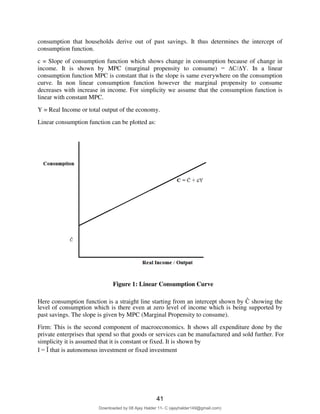
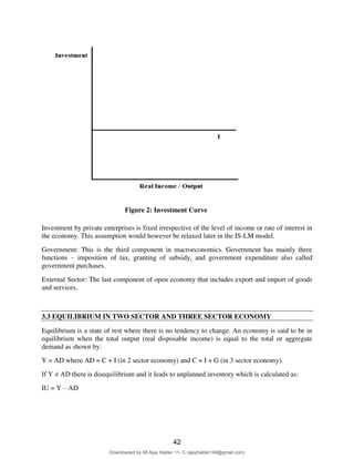
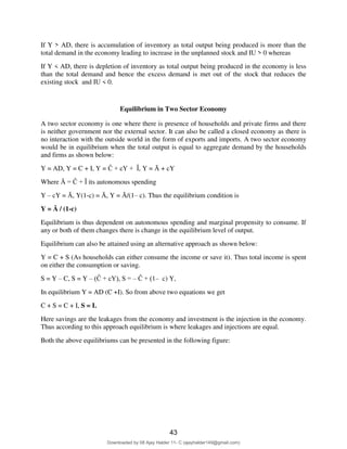
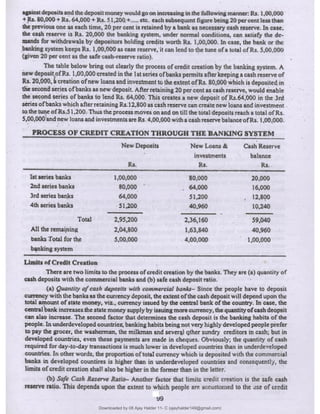
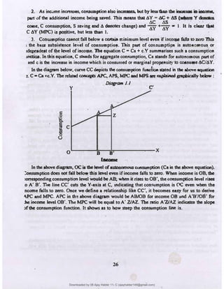
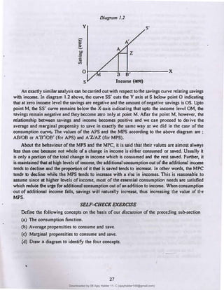
The document details principles of macroeconomics, specifically discussing national income accounting, GDP determinants, and the consumption and saving functions. It includes theories related to consumption such as the absolute income hypothesis and relative income hypothesis, while also exploring factors influencing consumption rates and investment levels. Additionally, it emphasizes the roles of interest rates, price levels, income distribution, and consumer credit in determining consumption behavior.
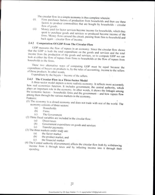
![Introduction
LESSON 3
DETERMINANTS OF INVESTMENT
As you already know, according to Keynes, the level of income in a capitalist economy
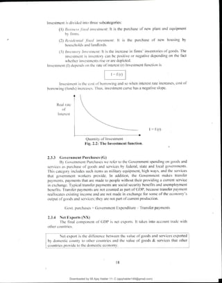
depends upon the level of aggregate demand. Aggregate demand originates from private
consumption expenditure, business investment expenditure, government expenditure and ellp(llt"
demand. Y01t have also seen that a change in any of the above items of expenditure results in a
much larger change in income through the multiplier effect. Out of these items of expenditure,
we have so far assumed investment as an autonomous quantity, dete.rmined independently and
outside the system. But now we relax that assumption and see how level•ofinwstment is determined
In the economic system. In this context, we discuss basically two theories of investment, the first
being the Keynesian concept of the Marginal Efficiency of Capital (MEC) and the second is the
Acceleration Principle.
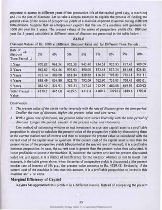
Discounting Future Values
Before explaining the concept of MEC, we discuss first the principle of discounting in the
context of capital goods. Capital goods a:re durable-use goods.which aid production over a number
ofyears. Returns from these capital goods are spread overthe whole of their useful lives. Therefore,
investment in capital goods necessitates estimation of their prospective yields. Prospective yield
from a capital good is MPP x MR minus all variable costs (except interest and depreciation), where
MPP. is·margiral physical product and MR is marginal re�enue. While yields obtainablefrom the
use ofa-capital good arefaJure ,quantities, the cos/ ofa capital asset is payable al present. So
long as we have a positive rate ofinterest, amounts available infuture are worth less at present.
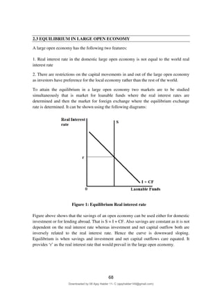
Therefore, we cannot comparefuture quan1l1ies (prospective yields) with present cost. We have
t9 calculate the present value of the sernes of prospective yields to make them comparable with
the cost of the capital good in question. For example, if.the present market rate of interest is I0%
p.a., Rs. I000 lent out today would grow to Rs. 1210 in 2 years [(IOOO (110/100)1] and to Rs.
13.31 in 3 years [IOOOx(t.l)']. Thus at the currP�• market rate of interest of 10¾, the present
value of Rs. 1331 obtainable after 3 years is Rs. IWO [That is 1331 x (1001110)'�I000] and the
present value of Rs. 1210 obtainable after + years is also Rs. I000 [that is 121 0•(I001110)']. We
call this "disco,mling" thefaJure values, the process through which a fat11re quantify shrinks
when converted into present value. This discounting process is Si{Tlply the reverse of/he process
through which any present quantity grows at a compound rote when carried intofuture. We can
similarly calculate the present vaJue of a wlole series of prospective yields available at different
points of time in future.
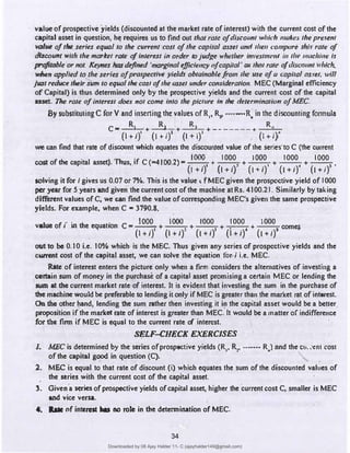
The general formula for finding the present value of any future income-stream is :
C
= R1 • + R2 + R, +-------+ R.
(1+1)
1
(l+i)' (l+i)
3
(l+i)"
In this equati�n, V is the present discounted value, R,, R,, •···R, are prospective -returns
32
Downloaded by 08 Ajay Halder 11- C (ajayhalder149@gmail.com)
lOMoARcPSD|24060133](https://image.slidesharecdn.com/unit-1-5-principles-of-macroeconomics-230604025115-a9a97376/85/unit-1-5-principles-of-macroeconomics-pdf-33-320.jpg)