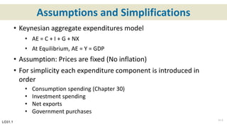
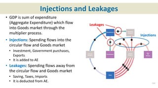
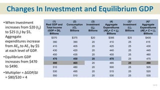
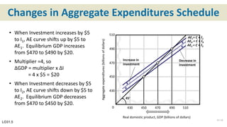
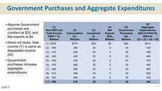
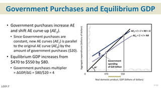
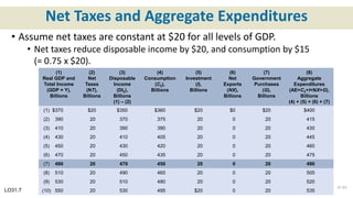
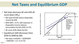
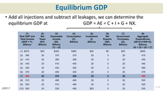
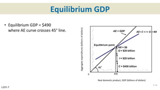
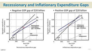
The document summarizes key concepts from Chapter 31 of an economics textbook on the aggregate expenditures model. It introduces the model's assumptions, components of aggregate expenditures (C + I + G + NX), and how equilibrium GDP is achieved when aggregate expenditures equal real GDP. It explains how changes in investment, net exports, government purchases affect the aggregate expenditures schedule and equilibrium GDP. The multiplier effect of changes in investment on equilibrium GDP is also discussed.

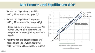


![Tahreem_Kousar_EconomicsSSSSSSSS_file[1].pptx](https://cdn.slidesharecdn.com/ss_thumbnails/tahreemkousareconomicsfile1-250617080609-d0ff08be-thumbnail.jpg?width=640&height=640&fit=bounds)


