![An Artificial Immune Network for Multimodal Function Optimization on Dynamic Environments Fabricio Olivetti de França LBiC/DCA/FEEC State University of Campinas (Unicamp) PO Box 6101, 13083-970 Campinas/SP, Brazil Phone: +55 19 3788-3885 [email_address] Fernando J. Von Zuben LBiC/DCA/FEEC State University of Campinas (Unicamp) PO Box 6101, 13083-970 Campinas/SP, Brazil Phone: +55 19 3788-3885 [email_address] Leandro Nunes de Castro Research and Graduate Program in Computer Science, Catholic University of Santos, Brazil. Phone/Fax: +55 13 3226 0500 [email_address]](https://image.slidesharecdn.com/doptleve-124042264675-phpapp02/85/An-Artificial-Immune-Network-for-Multimodal-Function-Optimization-on-Dynamic-Environments-1-320.jpg)
![An Artificial Immune Network for Multimodal Function Optimization on Dynamic Environments Fabricio Olivetti de França LBiC/DCA/FEEC State University of Campinas (Unicamp) PO Box 6101, 13083-970 Campinas/SP, Brazil Phone: +55 19 3788-3885 [email_address] Fernando J. Von Zuben LBiC/DCA/FEEC State University of Campinas (Unicamp) PO Box 6101, 13083-970 Campinas/SP, Brazil Phone: +55 19 3788-3885 [email_address] Leandro Nunes de Castro Research and Graduate Program in Computer Science, Catholic University of Santos, Brazil. Phone/Fax: +55 13 3226 0500 [email_address]](https://image.slidesharecdn.com/doptleve-124042264675-phpapp02/75/An-Artificial-Immune-Network-for-Multimodal-Function-Optimization-on-Dynamic-Environments-1-2048.jpg)


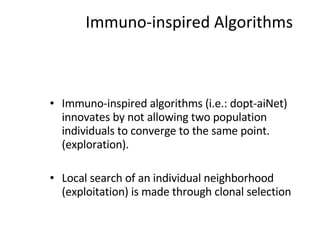


![dopt-aiNet Function [C] = dopt-aiNet(Nc,range, σ s,f,max_cells) C = random(range) While stopping criterion is not met do fit = f(C) C’ = clone(C,Nc) C’ = mutate(C’,f) C’ = one-dimensional(C’,f) C = clonal_selection(C,C’); C = gene_duplication(C,f) For each cell c from C do , If c’ is better than c, c.rank = c.rank + 1 c = c’ Else c.rank = c.rank – 1 End If c.rank == 0, Mem = [Mem, c] End End Avg = average(f(C)) If the average error does not stagnate return to the beginning of the loop else cell_line_suppress(C, σ s) C = [C; random(range)] End If size(C) > max_cells, suppress_fitness(C) End End End](https://image.slidesharecdn.com/doptleve-124042264675-phpapp02/85/An-Artificial-Immune-Network-for-Multimodal-Function-Optimization-on-Dynamic-Environments-36-320.jpg)


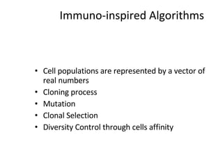
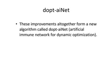
![Numerical Experiments Function Initialization Range Problem Dimension (N) f 1 [-500, 500] N 30 f 2 [-5.12, 5.12] N 30 f 3 [-32, 32] N 30 f 4 [-600, 600] N 30 f 5 [0, ] N 30 f 6 [-5, 5] N 100 f 7 [-5, 10] N 30 f 8 [-100, 100] N 30 f 9 [-10, 10] N 30 f 10 [-100, 100] N 30 f 11 [-100, 100] N 30](https://image.slidesharecdn.com/doptleve-124042264675-phpapp02/85/An-Artificial-Immune-Network-for-Multimodal-Function-Optimization-on-Dynamic-Environments-48-320.jpg)


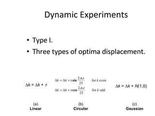
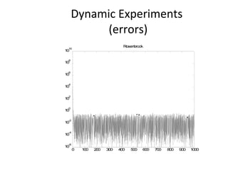
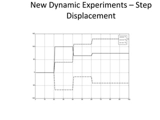
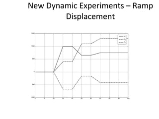
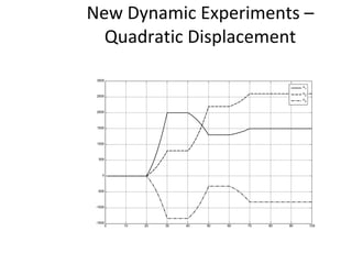
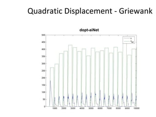
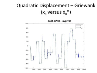
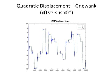
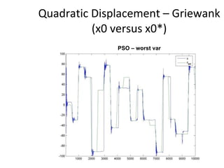
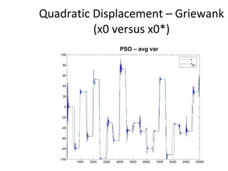
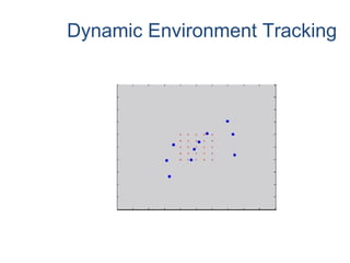
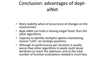
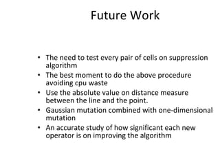


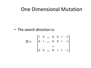
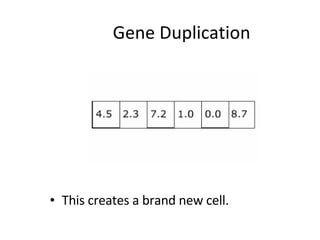
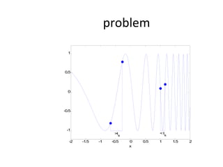
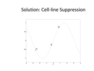
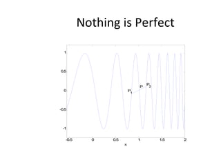
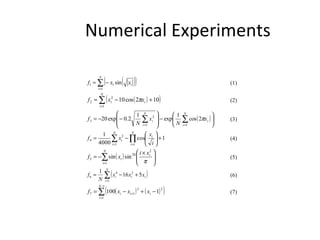
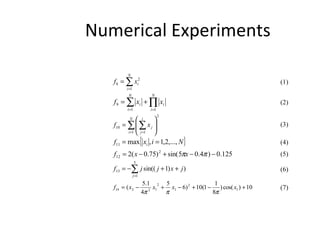
The document proposes an artificial immune network called dopt-aiNet for solving multimodal optimization problems in dynamic environments. dopt-aiNet is inspired by the immune system and uses clonal selection, mutation, and suppression techniques to maintain diversity and track moving optima. Numerical experiments show that dopt-aiNet outperforms other algorithms in terms of accuracy, convergence speed, and ability to track changing optima using fewer function evaluations. The paper discusses areas for future work such as improving suppression algorithms and studying the impact of different mutation operators.