This document discusses the formulation and types of optimization problems in evolutionary computation, emphasizing the importance of decision variables, objective functions, and constraints. It covers various optimization methods, including both derivative-based and derivative-free techniques, as well as challenges like multi-objective optimization and real-world applications. Additionally, it outlines different solution strategies, homework assignments, and examples relevant to optimization in engineering and management contexts.

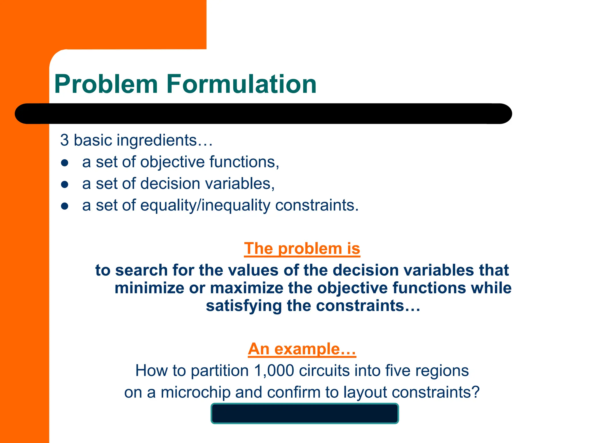
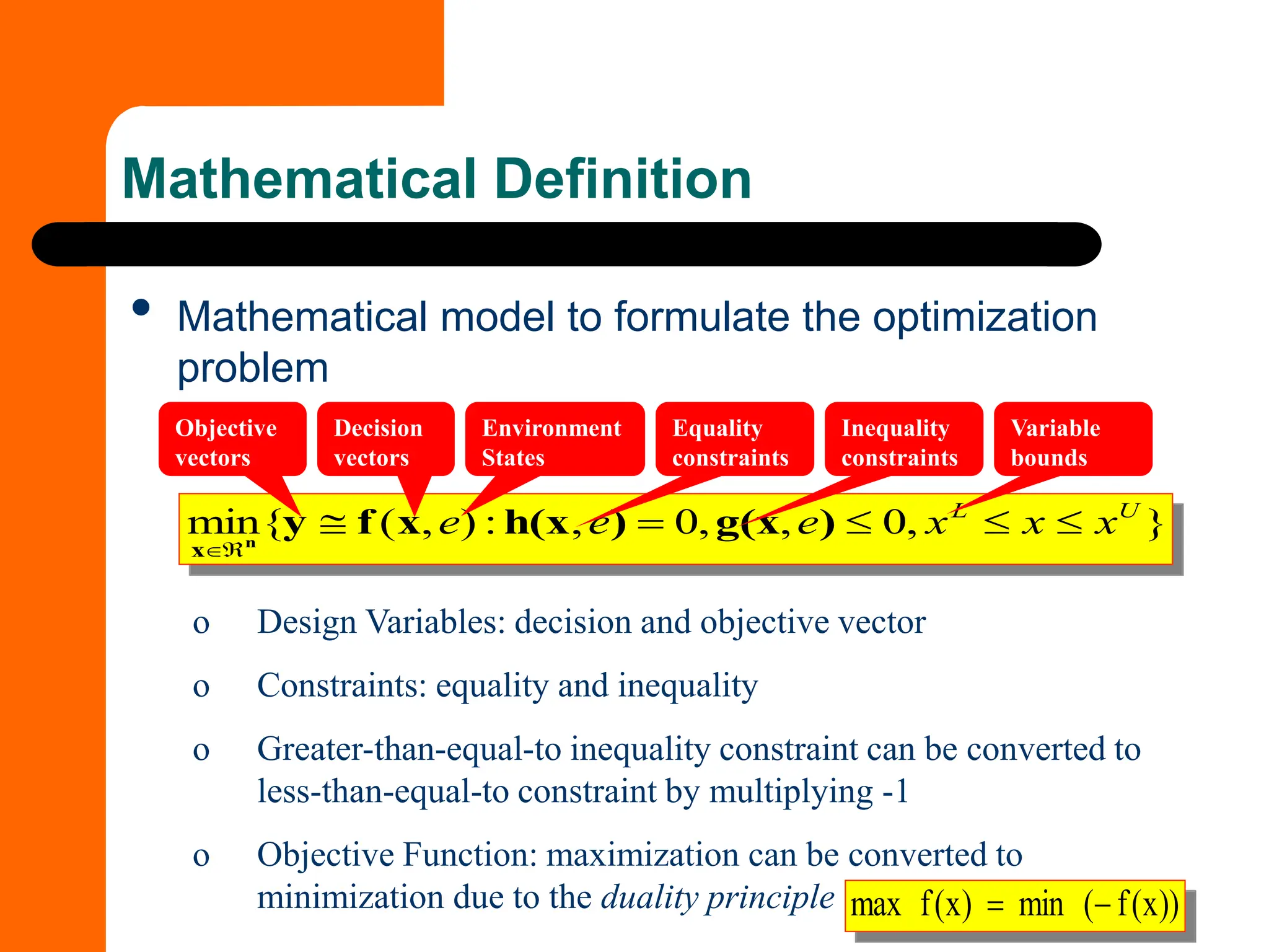
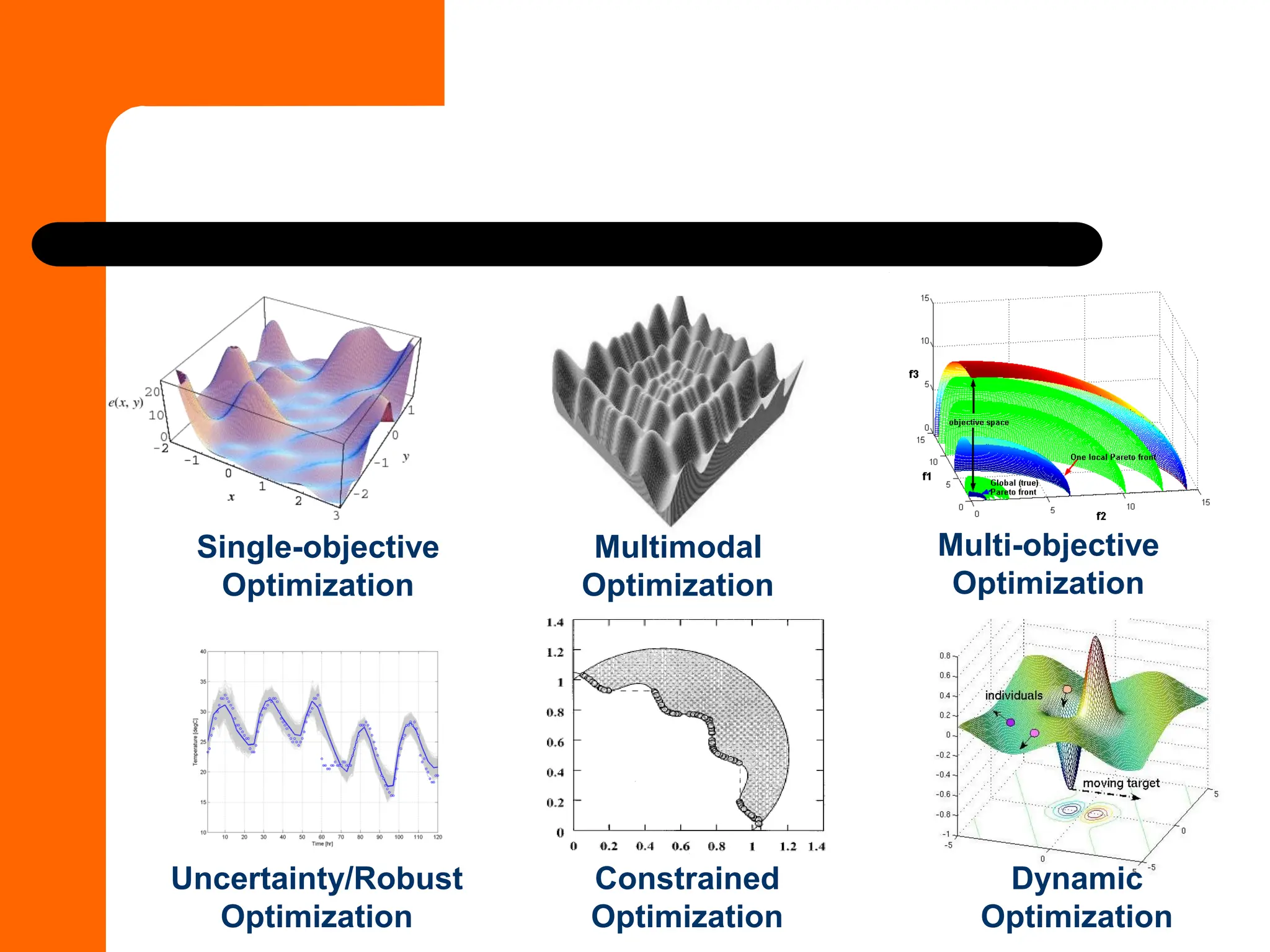
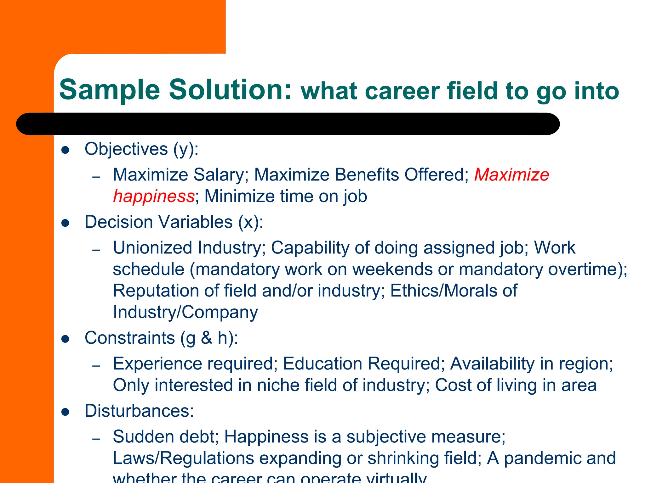
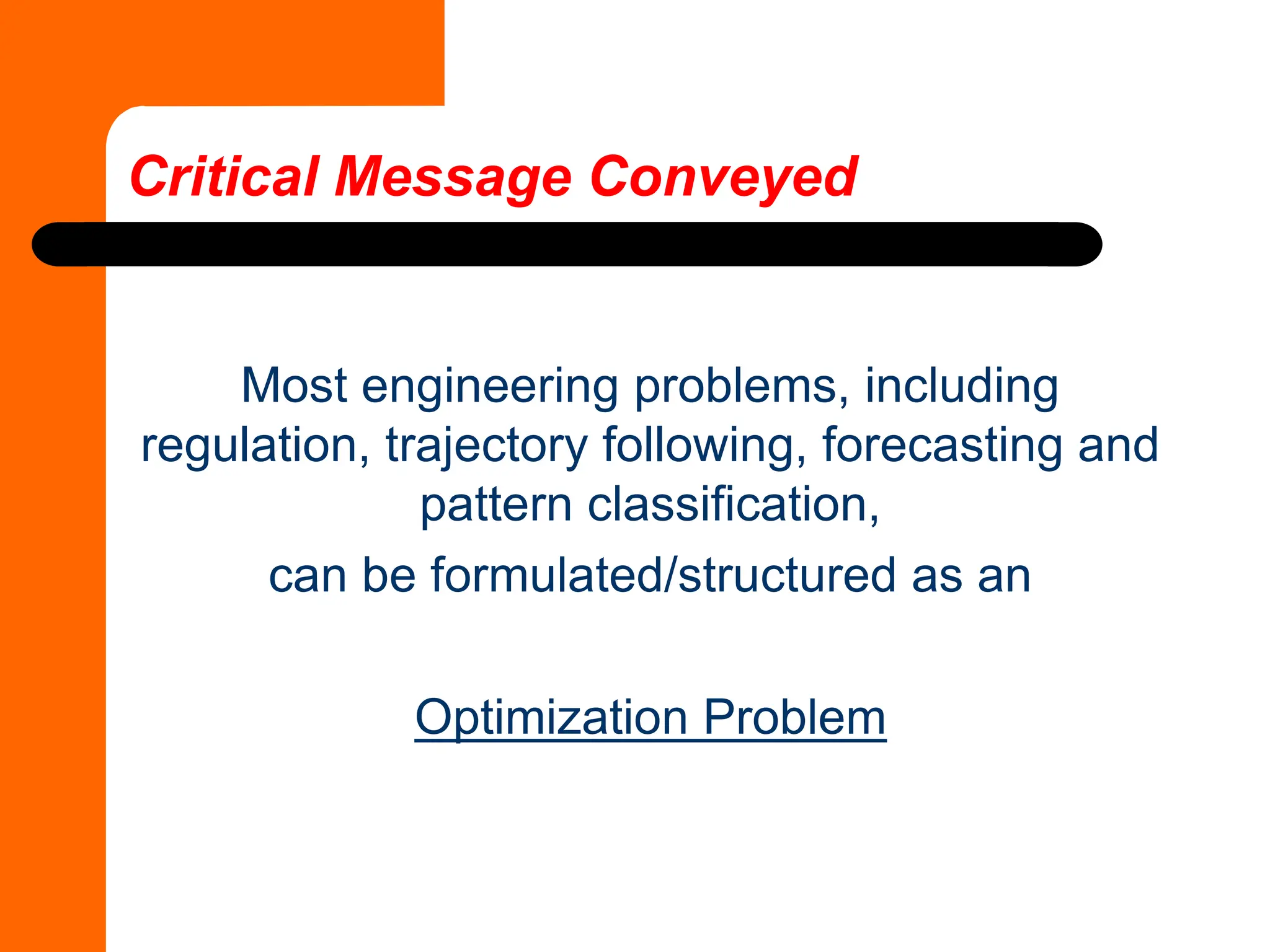
1. EVOLUTIONARY COMPUTATION
Lecture #3
8/23/2024
Fall 2024
ECEN/MAE 5773

2. OPTIMIZATION PROBLEMS

3. Problem Formulation
3 basic ingredients…
⚫ a set of objective functions,
⚫ a set of decision variables,
⚫ a set of equality/inequality constraints.
The problem is
to search for the values of the decision variables that
minimize or maximize the objective functions while
satisfying the constraints…
An example…
How to partition 1,000 circuits into five regions
on a microchip and confirm to layout constraints?
5^1000 = 9.33263619E698

4. Mathematical Definition
• Mathematical model to formulate the optimization
problem
}
,
0
,
,
0
,
:
)
,
(
{
min U
L
x
x
x
e
e
e 


=



)
g(x
)
h(x
x
f
y
n
x
))
x
(
f
(
min
)
x
(
f
max −
=
o Design Variables: decision and objective vector
o Constraints: equality and inequality
o Greater-than-equal-to inequality constraint can be converted to
less-than-equal-to constraint by multiplying -1
o Objective Function: maximization can be converted to
minimization due to the duality principle
Objective
vectors
Decision
vectors
Equality
constraints
Inequality
constraints
Variable
bounds
Environment
States

5. Single-objective
Optimization
Multimodal
Optimization
Constrained
Optimization
Multi-objective
Optimization
Dynamic
Optimization
Uncertainty/Robust
Optimization

6. Multiobjective Optimization
⚫ Optimization problems involve more than one objective
function
⚫ Very common, yet difficult problems in the field of science,
engineering, and business management
⚫ Nonconflicting objectives: achieve a single optimal solution
satisfies all objectives simultaneously
⚫ Competing objectives: cannot be optimized simultaneously
⚫ MOP– search for a set of “acceptable”– maybe only
suboptimal for one objective– solutions is our goal
⚫ In operation research/management terms – multiple criterion
decision making (MCDM)

7. Buying an Automobile
⚫ Objective = reduce
cost, while maximize
comfort
⚫ Which solution (1, A,
B, C, 2) is best ???
⚫ No solution from this
set makes both
objectives look better
than any other
solution from the set
⚫ No single optimal
solution
⚫ Trade off between
conflicting objectives-
cost and comfort

8. Engineering Design
Feasible region
Infesaible region

9. ⚫ Single objective optimization
is a degenerate case of
MOP
MOP is not a simple
extension of SOP
⚫ Multi-modal optimization is a
special case of MOP

10. Optimization Approaches
⚫ applicable only to SOP
⚫ search in a large space
⚫ Derivative-based optimization (gradient based)
– Capable of determining “search directions” according to an
objective function’s derivative information
– e.g., steepest descent method; Newton’s method; Newton-
Raphson method; and those in between such as conjugate
gradient method or Levenberg-Marquardt method
⚫ Derivative-free optimization
– e.g., simulated annealing; genetic algorithm; random search
method; downhill simplex search
– For both continuous and discrete optimization problems
– For combinatorial optimization problems

11. Common Characteristics
⚫ Derivative freeness
– these methods do not need functional derivative
information to search for a set of parameters that
minimize a given objective function. Instead, they
rely exclusively on repeated evaluations of the
objective function. The subsequent search
direction after each evaluation follows certain
heuristic guidelines.

12. ⚫ Intuitive guidelines
– The guidelines followed by these search
procedures are usually based on “simple,”
“heuristic” concepts. Some of these concepts are
motivated by so-called “nature’s wisdom,” such as
evolution and thermodynamics.
⚫ Slowness
– Without using derivatives, these methods are
bounded to be generally slower than derivative-
based optimization methods for continuous
optimization problems.

13. ⚫ Flexibility
– Derivative freeness also relieve the requirement
for differentiable objective functions, so we can
use as complex an objective function as a specific
application might need, without sacrificing too
much in extra coding and computation time.

14. ⚫ Randomness
– All of these methods (except standard downhill
simplex) are stochastic, which means that they all use
random number generators in determining subsequent
search directions. This element of randomness usually
gives rise to the overly optimistic view that these
methods are “global optimizers” that will find a global
optimum given enough computation time. In theory,
their random nature does make the probability of
finding an optimal solution nonzero over a fix amount
of computation time. In practice, however it might take
a considerable amount of computation time, if not
forever, to find the optimal solution of a given problem.

18. ⚫ Iterative nature
– Unlike the linear least-squares estimator, these techniques are iterative
in nature, and we need certain stopping criteria to determine when to
terminate the optimization process
– Let k denote an iterative count and
fk denote the best objective function obtained at count k.
– Stopping criteria:
⚫ computation time: a designated amount of computation time or number of
iterations/function evaluation
⚫ optimization goal:
⚫ Minimization improvement:
⚫ Minimal relative improvement:


k
f


− −1
k
k f
f


−
−
−
1
1
k
k
k
f
f
f

19. ⚫ Analytic opacity
– It is difficult to do analytic studies of these methods, in part
because of their randomness and problem–specific nature.
Therefore, most of our knowledge about them is based on
empirical studies.

20. ⚫ Bundle methods Conjugate gradient method
⚫ Ellipsoid method Frank–Wolfe method
⚫ Gradient descent aka steepest descent or steepest ascent
⚫ Interior point methods
⚫ Line search - a technique for one dimensional optimization, usually used
as a subroutine for other, more general techniques.
⚫ Nelder-Mead method aka the Amoeba method
⚫ Newton's method Quasi-Newton methods
⚫ Simplex method
⚫ Subgradient method - similar to gradient method in case there are no
gradients
⚫ Constrained problems can often be transformed into unconstrained
problems with the help of Lagrange multipliers
Traditional Approaches

21. Heuristic Approaches
⚫ Ant colony optimization
⚫ Beam search
⚫ Cockroach algorithm
⚫ Differential Evolution
⚫ Evolution Strategy
⚫ Evolutionary Programming
⚫ Firefly algorithm
⚫ Genetic Algorithm
⚫ Hill climbing
⚫ Particle Swarm Optimization
⚫ Simulated annealing
⚫ Tabu search
⚫ Artificial Immune System
• Bat algorithm
• Bee algorithm
• Cuckoo search
• Dynamic relaxation
• Firework algorithm
• Filled function method
• Harmony search
• IOSO
• Quantum annealing
• Stochastic tunneling

22. Some Approaches
⚫ Random Search
– simplest and most intuitive
⚫ Downhill Simplex
– based on heuristic adaptation of a geometric object (a
simplex) to explore a performance landscape
⚫ Simulated Annealing
– originated in the annealing process found in the
thermodynamics and metallurgy
⚫ Genetic Algorithm
– based on the concept of natural selection through the
“survival of the fittest” law
⚫ Ant Colony
– inspired by the natural metaphor that real ants are capable
of finding the shortest path from a food source to their nest
without using visual cues by exploiting pheromone
information

23. ⚫ Random search
⚫ Greedy search (downhill)
1. Randomize the starting configuration
2. If possible, find a better configuration by making random changes to
the current configuration
3. Make this better configuration the current one, then go to step 2
4. If a better configuration is not found after a reasonable effort, conclude
that you have obtained a local minimum, save it in the variable
OPTIMUM (easily trapped in local minima)
5. Repeat from step 1, replacing OPTIMUM if appropriate, until your
patience or computing resource are exhausted; hope that the final
value of OPTIMUM is global.
⚫ Simulated annealing
– Allow perturbations to move uphill in a controlled fashion to escape
from local minima

24. Concerning Issues
⚫ Existness of the global optimum
⚫ Uniqueness of the global optimum
⚫ Convergence of the stochastic algorithm
⚫ Convergence speed of the algorithm
⚫ Continuation of the mapping from decision variables to
objective functions
⚫ Noise in fitness function
and evaluation
⚫ Fuzziness in fitness function
and evaluation

25. Homework #1
• Post in Canvas
Assigned: 8/23/24;
Due: 8/30/24

26. ⚫ Homework is due before midnight on the day.
⚫ Every homework solution in a SINGLE standalone PDF
file is to be turned in through Canvas website.
⚫ Using a scanner as needed, such as Adobe scan or
Scanner app from IOS and Android via your phone. Do
assure the pdf file created present a quality (readable)
output.
Policy on Homework Submitted

27. ⚫ Energy Distribution in an Iron & Steel Factory
Coking
coke oven
S inter
machine
 
Casting
caster

Steelmaking
converter
electric furnace

Gas station E nergy managementcenter
steam

O2
N2
iron ore
Mine
coal


Electric power

Rolling
heating furnace
hot roller
cold roller
Ironmaking
pellet
coke

COG
BFG LDG
Steam
N2
Steam
N2
O2 ,N2
steam
O2 ,N2
Blast
furnace
BFG COG LDG
Sample Solution #1

28. To improve the energy utilization level, the goal of energy
distribution problem is to minimize the total energy cost by
determining the amount of energy supply to all processes,
considering energy supply, holding capacity, regeneration, and
conversion.
1 0
1
I
i
i
f c x
=
= 
2 1
f c z
=
3 2
f c w
=
4
1 1
max{0, ( )}
I I
i i
i i
f h H y z x w
= =
= + + − −
 
Objective functions to be minimized:
gas consumption cost
gas purchase cost
emission cost
gas inventory holding cost
“Soft constraint handling for a real-world multi-objective energy distribution problem,” Zhang
Y., Yen G.G. and Tang L., International Journal on Production Research, 58(19), 2020, pp.
6061-6077.

29. Possible Disturbances:
sensor measurements
model uncertainties
fluctuation of energy market

30. gas supply capacity constraint
regenerated secondary energy, the purchased energy,
and the decrease of storage
lower bound gas consumption ratio constraint
upper bound gas consumption ratio constraint
lower bound gas pipeline inventory capacity
(pressure) constraint
upper bound gas pipeline pressure constraint
lower bound gas regeneration capacity constraint
upper bound gas regeneration capacity constraint
additional purchase constraint
gas emission limit constraint
nonnegative value fields
Constraints Considered

31. ⚫ Pickup and Delivery Problem with Time
Windows and Demands (PDP-TW-D)
o PDP-TW-D is a combinatorial optimization problem of finding a set of optimal
routes for a fleet of vehicles in order to serve given transportation requests.
o Each transportation request is defined by a pickup location, a delivery
location, goods to be transported, a pickup time window and a delivery time
window.
o Each pickup/delivery location needs to be visited by a vehicle within a certain
time window.
o Each vehicle has a capacity to load goods and follows an assigned route (i.e., a
sequence of pickup/delivery locations) by loading goods at pickup locations
and unloading them at delivery locations.
o Examples: military/civilian airlift and sealift, parcel services, taxi dispatching,
shared taxi services, school bus routing, dial-a-ride services, food delivery, and
etc.
Sample Solution #2

32. f i v e c o n f l i c t o b j e c t i v e s :
T h r e e c o n s t r a i n t s :

33. Problem at hand- which restaurant to go for the dinner?
⚫ Objectives: 1) maximize food quality; 2) maximize portion
serving size; 3) minimize driving distance or time
⚫ Decision Variables: 1) cost; 2) reputation/rating from
Yelp; 3) business hours; 4) culinary style
⚫ Constraints: 1) cost should be mid-range/affordable for a
college student; 2) only interested in 2-star or 3-star; 3)
preferable Mexican or Italian food
⚫ Disturbances: 1) possible construction on the shortest
route; 2) subjective measure for food quality
Sample Solution #3

34. ⚫ Objectives (y):
– Maximize Salary; Maximize Benefits Offered; Maximize
happiness; Minimize time on job
⚫ Decision Variables (x):
– Unionized Industry; Capability of doing assigned job; Work
schedule (mandatory work on weekends or mandatory overtime);
Reputation of field and/or industry; Ethics/Morals of
Industry/Company
⚫ Constraints (g & h):
– Experience required; Education Required; Availability in region;
Only interested in niche field of industry; Cost of living in area
⚫ Disturbances:
– Sudden debt; Happiness is a subjective measure;
Laws/Regulations expanding or shrinking field; A pandemic and
Sample Solution: what career field to go into

35. Most engineering problems, including
regulation, trajectory following, forecasting and
pattern classification,
can be formulated/structured as an
Optimization Problem
Critical Message Conveyed