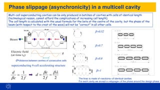
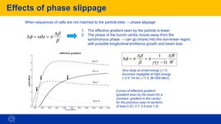
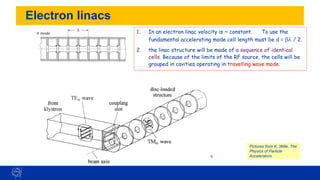
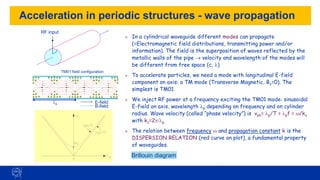
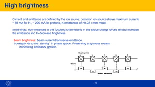
This document provides an overview of linear accelerators (linacs), explaining their basic structure, operational principles, and types, including continuous wave and pulsed linacs. It discusses the physics behind acceleration in periodic structures and the differences between linear and circular accelerators, including practical applications in particle physics and medical fields. Additionally, it covers more complex topics like wave propagation, phase slippage, and specific examples of linac implementations at CERN.

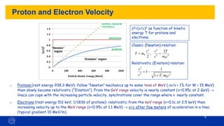
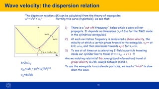
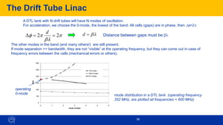
![Definitions
3
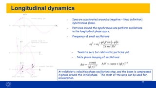
Linear accelerator: a device where charged particles acquire energy moving on a linear path
RF linear accelerator: acceleration is provided by time-varying electric fields (i.e. excludes
electrostatic accelerators)
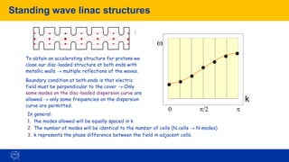
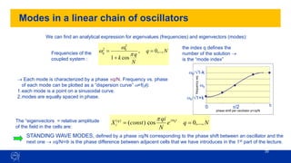
A few definitions:
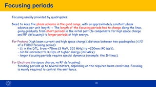
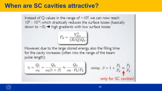
➢CW (Continuous wave) linacs when the beam bunches come continuously out of the linac;
➢Pulsed linac when the beam is produced in pulses: t pulse length, fr repetition frequency, beam
duty cycle t × fr (%)
➢ Main parameters: E kinetic energy of the particles coming out of the linac [MeV]
I average current during the beam pulse [mA] (different from average
current and from bunch current !)
P beam power = electrical power transferred to the beam during acceleration
P [W] = Vtot × I = E [eV] × I [A] × duty cycle](https://image.slidesharecdn.com/doctoralschool0422linacs-241220093326-062733ae/85/doctoral_school_04_22_linacsssssssssssss-3-320.jpg)
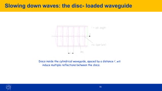

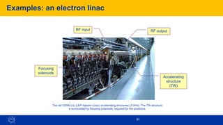
![44
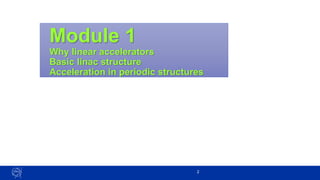
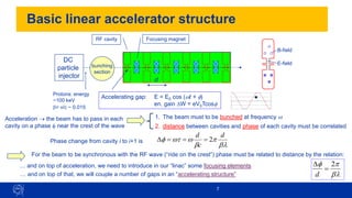
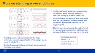
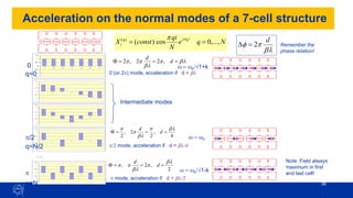
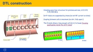
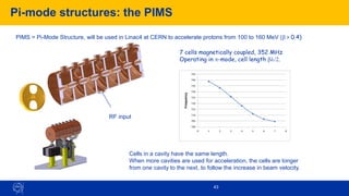
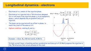
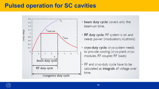
Sequence of PIMS cavities
Cells have same length inside a cavity (7 cells) but increase from one cavity to the next.
At high energy (>100 MeV) beta changes slowly and phase error (“phase slippage”) is small.
0
1
0 100 200 300 400
Kinetic Energy[MeV]
(v/c)^2
100 MeV,
128 cm
160 MeV,
155 cm
Focusing quadrupoles
between cavities
PIMS range](https://image.slidesharecdn.com/doctoralschool0422linacs-241220093326-062733ae/85/doctoral_school_04_22_linacsssssssssssss-44-320.jpg)

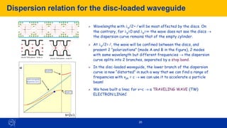
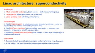
![68
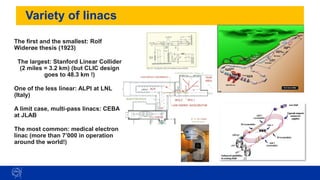
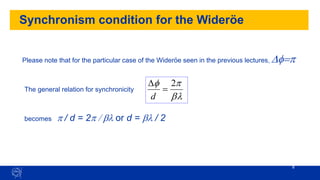
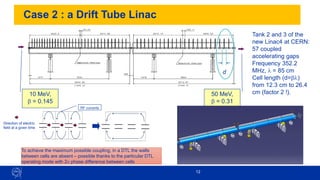
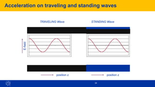
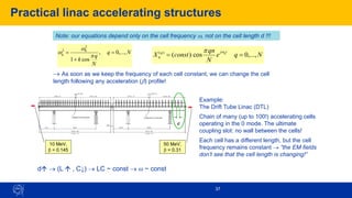
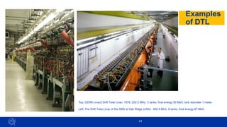
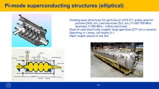
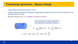
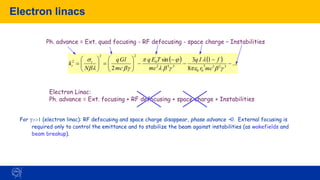
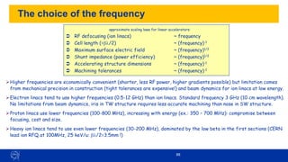
High-intensity protons – the case of Linac4
Example: beam dynamics design for Linac4@CERN.
High intensity protons (60 mA bunch current, duty cycle could go up to 5%), 3 - 160 MeV
Beam dynamics design minimising emittance growth and halo development in order to:
1. avoid uncontrolled beam loss (activation of machine parts)
2. preserve small emittance (high luminosity in the following accelerators)
Transverse (x) r.m.s. beam envelope along Linac4
0
0.001
0.002
0.003
0.004
0.005
10 20 30 40 50 60 70 80
distance from ion source [m]
x_rms
beam
size
[m]
DTL : FFDD and FODO
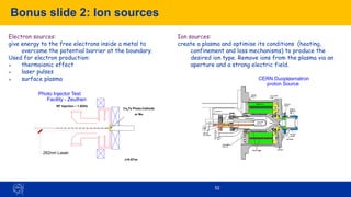
CCDTL : FODO PIMS : FODO](https://image.slidesharecdn.com/doctoralschool0422linacs-241220093326-062733ae/85/doctoral_school_04_22_linacsssssssssssss-68-320.jpg)
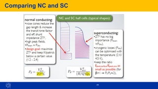
![69
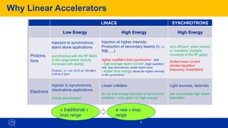
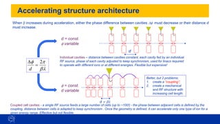
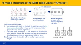
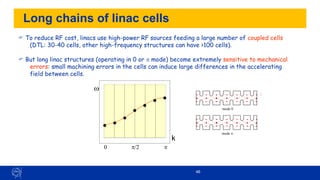
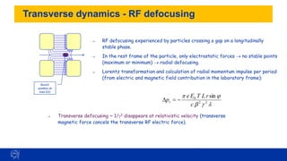
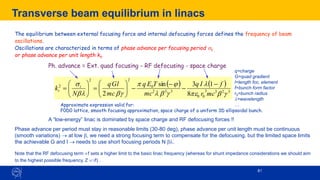
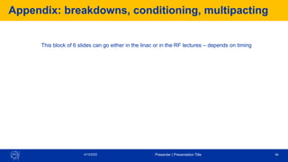
Beam Optics Design Guidelines
Prescriptions to minimise emittance growth and halo formation:
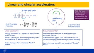
1. Keep zero current phase advance always below 90º, to avoid resonances
2. Keep longitudinal to transverse phase advance ratio 0.5-0.8, to avoid emittance exchange
3. Keep a smooth variation of transverse and longitudinal phase advance per meter.
4. Keep sufficient safety margin between beam radius and aperture
Transverse r.m.s. emittance and phase advance along Linac4 (RFQ-DTL-CCDTL-PIMS)
0
20
40
60
80
100
120
140
160
180
200
220
0 10 20 30 40 50 60 70
position [m]
phase
advance
per
meter
kx
ky
kz
2.00E-07
2.50E-07
3.00E-07
3.50E-07
4.00E-07
4.50E-07
0 10 20 30 40 50 60 70 80
100% Normalised RMS transverse emittance (PI m rad)
x
y
transition
transition](https://image.slidesharecdn.com/doctoralschool0422linacs-241220093326-062733ae/85/doctoral_school_04_22_linacsssssssssssss-69-320.jpg)
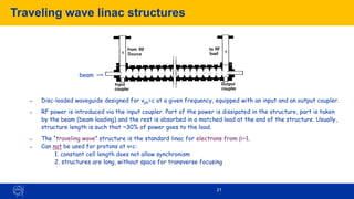
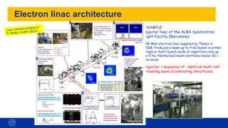
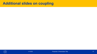
![76
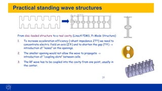
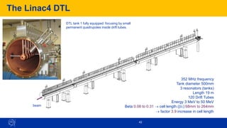
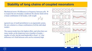
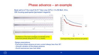
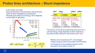
Proton linac architecture – cell length, focusing period
Injector
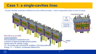
EXAMPLE: the Linac4 project at CERN. H-, 160 MeV energy, 352 MHz.
A 3 MeV injector + 22 multi-cell standing wave accelerating structures of 3 types
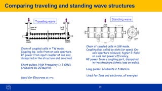
Two basic principles to remember:
1. As beta increases, phase error
between cells of identical length
becomes small → we can have short
sequences of identical cells (lower
construction costs).
2. As beta increases, the distance
between focusing elements can increase
(more details in 2nd lecture!).
DTL: every cell is different, focusing quadrupoles in each drift tube
CCDTL: sequences of 2 identical cells, quadrupoles every 3 cells
PIMS: sequences of 7 identical cells, quadrupoles every 7 cells
Section Output
Energy
[MeV]
Number of
consecutive
identical cells
Distance
between
quadrupoles
RFQ 3 1 -
DTL 50 1 b
CCDTL 100 3 4 b
PIMS 160 7 5 b](https://image.slidesharecdn.com/doctoralschool0422linacs-241220093326-062733ae/85/doctoral_school_04_22_linacsssssssssssss-76-320.jpg)
![High Energy Linacs
78
Superconducting Proton Linac a CERN project for extending Linac4 up to 5 GeV energy
Section Output
Energy
[MeV]
Lattice Number of
RF gaps
between
quadrupoles
Number of
RF gaps
per period
Number of
consecutive
identical
cells
DTL 50 F0D0 1 2 1
CCDTL 102 F0D0 3 6 3
PIMS 160 F0D0 12 24 12
Low b 750 FD 15 15 300
High b / 1 2500 FD 35 35
920
High b / 2 5000 F0D0 35 70
low-beta: 20 cryo-modules with 3 cavities/cryo-module
high-beta -FD: 13 cryo-modules with 8 cavities/module
high-beta -FODO: 10 cryo-modules with 8 cavities/module](https://image.slidesharecdn.com/doctoralschool0422linacs-241220093326-062733ae/85/doctoral_school_04_22_linacsssssssssssss-78-320.jpg)
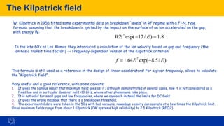
![Transition warm/cold
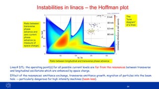
87
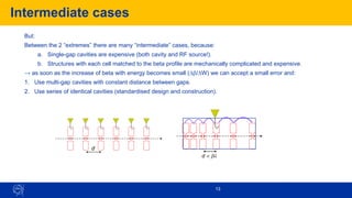
The RFQ must be normal conducting (construction problems / inherent beam loss).
Modern high-energy (>200 MeV) sections should be superconducting.
But where is the optimum transition energy between normal and superconducting?
The answer is in the cost → the economics has to be worked out correctly !
SNS
JPARC
Linac4/SPL
ESS
0
50
100
150
200
250
300
350
400
450
1 10 100
Project Duty Cycle
[%]
Transition
Energy [MeV]
SNS 6 186
JPARC 2.5 400
Linac4/SPL 4 160
ESS 4 50
Project-X 100 10
EUROTRANS 100 5
EURISOL 100 5
IFMIF/EVEDA 100 5
Overview of warm/cold transition
energies for linacs (operating
and in design)
Duty cycle [%]
Energy
[MeV]
90](https://image.slidesharecdn.com/doctoralschool0422linacs-241220093326-062733ae/85/doctoral_school_04_22_linacsssssssssssss-87-320.jpg)
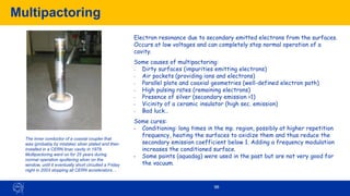
![Linac architecture: optimum gradient (NC)
89
The cost of a linear accelerator is made of 2 terms:
• a “structure” cost proportional to linac length
• an “RF” cost proportional to total RF power
P
C
l
C
C RF
s +
=
Cs, CRF unit costs (€/m, €/W)
T
E
C
T
E
C
C RF
s 0
0
1
+
0
20
40
60
80
100
120
5 15 25 35 45 55 65 75 85 95 105
E0 [MV/m]
Cost
Total cost
structure cost
RF cost
Example: for Linac4
Cs … ~200 kCHF/m
CRF…~0.6 CHF/W (recuperating LEP equipment)
E0T … ~ 3 – 4 MV/m
Note that the optimum design gradient (E0T) in a normal-conducting linac is
not necessarily the highest achievable (limited by sparking).
T
E
l 0
/
1
T
E
l
T
E
P 0
2
0 )
(
Overall cost is the sum of a structure term
decreasing with the gradient and of an RF
term increasing with the gradient → there is
an optimum gradient minimizing cost.
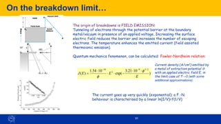
breakdown limit
optimum
gradient](https://image.slidesharecdn.com/doctoralschool0422linacs-241220093326-062733ae/85/doctoral_school_04_22_linacsssssssssssss-89-320.jpg)
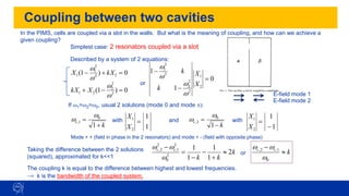
![More on coupling
- “Coupling” only when
the 2 resonators are
close in frequency.
- For f1=f2, maximum
spacing between the 2
frequencies (=kf0)
The coupling k is:
•Proportional to the 3rd power of slot length.
•Inv. proportional to the stored energies.
Solving the previous equations allowing a different frequency for each cell, we can plot the frequencies of the coupled
system as a function of the frequency of the first resonator, keeping the frequency of the second constant, for different
values of the coupling k.
170
180
190
200
210
220
230
170 180 190 200 210 220 230
f1c
f2c
f1c
f2c
f1c
f2c
120
140
160
180
200
220
240
260
280
120 140 160 180 200 220 240 260 280
Coupled
freqeuencies
[MHz]
Frequency f1 [MHz]
maximum
separation
when f1=f2
f1 f0
case of 3
different
coupling
factors
(0.1%, 5%,
10%)
For an elliptical coupling slot:
2
2
1
1
3
U
H
U
H
l
F
k
F = slot form factor
l = slot length (in
the direction of H)
H = magnetic field
at slot position
U = stored energy](https://image.slidesharecdn.com/doctoralschool0422linacs-241220093326-062733ae/85/doctoral_school_04_22_linacsssssssssssss-99-320.jpg)