An Introduction to Particle Accelerators

1. An Introduction to
Particle Accelerators
Erik Adli, University of Oslo/CERN
, University of Oslo/CERN
2009
Erik.Adli@cern.ch
v1.42 - short

2. LHC FIRST BEAM 10-sep-2008

3. Introduction
Part 1

4. Particle accelerators for HEP
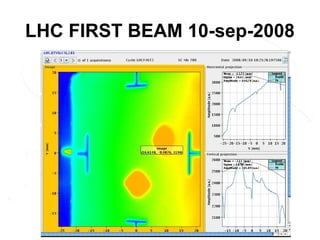
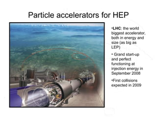
•LHC: the world
biggest accelerator,
both in energy and
size (as big as
LEP)
• Grand start-up
and perfect
functioning at
injection energy in
September 2008
•First collisions
expected in 2009

5. Particle accelerators for HEP
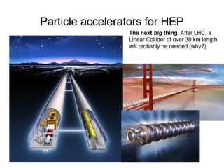
The next big thing. After LHC, a
Linear Collider of over 30 km length,
will probably be needed (why?)

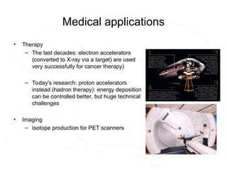
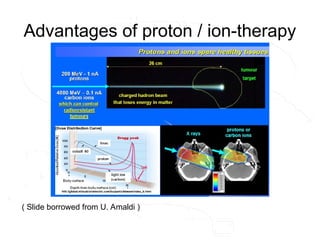
6. Medical applications
• Therapy
– The last decades: electron accelerators
(converted to X-ray via a target) are used
very successfully for cancer therapy)
– Today's research: proton accelerators
instead (hadron therapy): energy deposition
can be controlled better, but huge technical
challenges
• Imaging
– Isotope production for PET scanners

7. Advantages of proton / ion-therapy
( Slide borrowed from U. Amaldi )

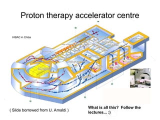
8. Proton therapy accelerator centre
( Slide borrowed from U. Amaldi )
What is all this? Follow the
lectures... :)
HIBAC in Chiba

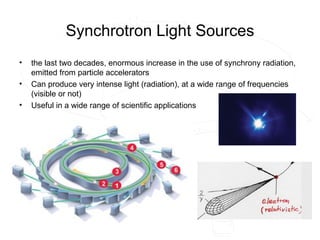
9. Synchrotron Light Sources
• the last two decades, enormous increase in the use of synchrony radiation,
emitted from particle accelerators
• Can produce very intense light (radiation), at a wide range of frequencies
(visible or not)
• Useful in a wide range of scientific applications

10. Thorium - Accelerator Driven Systems

11. Basic concepts
Part 2

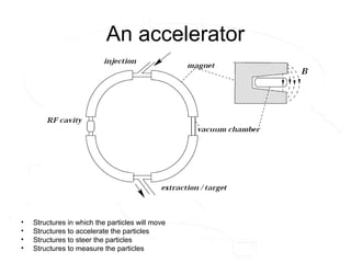
12. An accelerator
• Structures in which the particles will move
• Structures to accelerate the particles
• Structures to steer the particles
• Structures to measure the particles

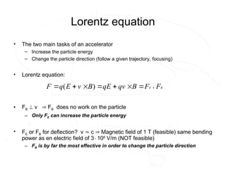
13. Lorentz equation
• The two main tasks of an accelerator
– Increase the particle energy
– Change the particle direction (follow a given trajectory, focusing)
• Lorentz equation:
• FB  v  FB does no work on the particle
– Only FE can increase the particle energy
• FE or FB for deflection? v  c  Magnetic field of 1 T (feasible) same bending
power as en electric field of 3108
V/m (NOT feasible)
– FB is by far the most effective in order to change the particle direction
B
E F
F
B
v
q
E
q
B
v
E
q
F
















 )
(

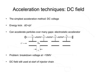
14. Acceleration techniques: DC field
• The simplest acceleration method: DC voltage
• Energy kickE=qV
• Can accelerate particles over many gaps: electrostatic accelerator
• Problem: breakdown voltage at ~10MV
• DC field still used at start of injector chain

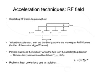
15. Acceleration techniques: RF field
• Oscillating RF (radio-frequency) field
• “Widerøe accelerator”, after the pioneering work of the Norwegian Rolf Widerøe
(brother of the aviator Viggo Widerøe)
• Particle must sees the field only when the field is in the accelerating direction
– Requires the synchronism condition to hold: Tparticle =½TRF
• Problem: high power loss due to radiation
vT
L )
2
/
1
(


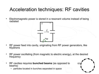
16. Acceleration techniques: RF cavities
• Electromagnetic power is stored in a resonant volume instead of being
radiated
• RF power feed into cavity, originating from RF power generators, like
Klystrons
• RF power oscillating (from magnetic to electric energy), at the desired
frequency
• RF cavities requires bunched beams (as opposed to coasting
beams)
– particles located in bunches separated in space

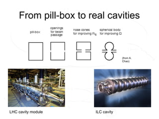
17. From pill-box to real cavities
LHC cavity module ILC cavity
(from A.
Chao)

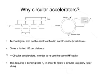
18. Why circular accelerators?
• Technological limit on the electrical field in an RF cavity (breakdown)
• Gives a limited E per distance
  Circular accelerators, in order to re-use the same RF cavity
• This requires a bending field FB in order to follow a circular trajectory (later
slide)

19. The synchrotron
• Acceleration is performed by RF cavities
• (Piecewise) circular motion is ensured by a guide field FB
• FB : Bending magnets with a homogenous field
• In the arc section:
• RF frequency must stay locked to the revolution frequency of a particle
(later slide)
• Synchrotrons are used for most HEP experiments (LHC, Tevatron, HERA,
LEP, SPS, PS) as well as, as the name tells, in Synchrotron Light Sources
(e.g. ESRF)
]
/
[
]
[
3
.
0
]
[
1
1
F 1
2
B
c
GeV
p
T
B
m
p
qB
v
m 



 




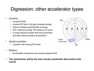
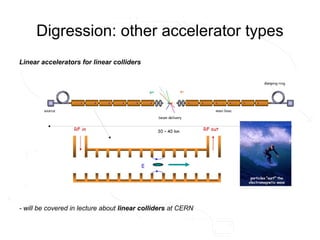
20. Digression: other accelerator types
• Cyclotron:
– constant B field
– constant RF field in the gap increases energy
– radius increases proportionally to energy
– limit: relativistic energy, RF phase out of synch
– In some respects simpler than the synchrotron,
and often used as medical accelerators
• Synchro-cyclotron
– Cyclotron with varying RF phase
• Betatron
– Acceleration induced by time-varying magnetic field
• The synchrotron will be the only circular accelerator discussed in this
course

21. Digression: other accelerator types
Linear accelerators for linear colliders
- will be covered in lecture about linear colliders at CERN

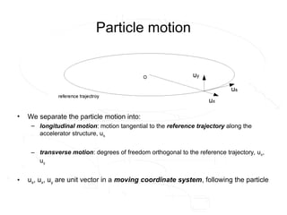
22. Particle motion
• We separate the particle motion into:
– longitudinal motion: motion tangential to the reference trajectory along the
accelerator structure, us
– transverse motion: degrees of freedom orthogonal to the reference trajectory, ux,
uy
• us, ux, uy are unit vector in a moving coordinate system, following the particle

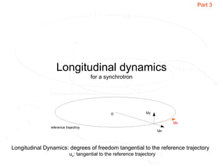
23. Longitudinal dynamics
for a synchrotron
Longitudinal Dynamics: degrees of freedom tangential to the reference trajectory
us: tangential to the reference trajectory
Part 3

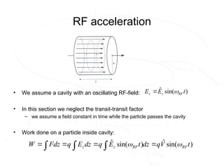
24. RF acceleration
• We assume a cavity with an oscillating RF-field:
• In this section we neglect the transit-transit factor
– we assume a field constant in time while the particle passes the cavity
• Work done on a particle inside cavity:
)
sin(
ˆ t
E
E RF
z
z 

)
sin(
ˆ
)
sin(
ˆ t
V
q
dz
t
E
q
dz
E
q
Fdz
W RF
RF
z
z 
 


 



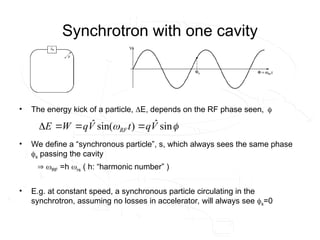
25. Synchrotron with one cavity
• The energy kick of a particle, E, depends on the RF phase seen
• We define a “synchronous particle”, s, which always sees the same phase
s passing the cavity
 RF =h rs ( h: “harmonic number” )
• E.g. at constant speed, a synchronous particle circulating in the
synchrotron, assuming no losses in accelerator, will always see s=0

 sin
ˆ
)
sin(
ˆ V
q
t
V
q
W
E RF 




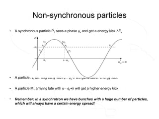
26. Non-synchronous particles
• A synchronous particle P1 sees a phase s and get a energy kick Es
• A particle N1 arriving early with  s will get a lower energy kick
• A particle M1 arriving late with  s will get a higher energy kick
• Remember: in a synchrotron we have bunches with a huge number of particles,
which will always have a certain energy spread!

27. Frequency dependence on energy
• In order to see the effect of a too low/high E, we need to study the
relation between the change in energy and the change in the revolution
frequency : "slip factor")
• Two effects:
1. Higher energy  higher speed (except ultra-relativistic)
2. Higher energy  larger orbit “Momentum compaction”
p
dp
f
df r
r
/
/


R
c
fr


2


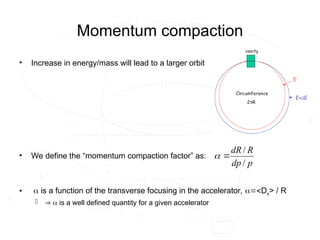
28. Momentum compaction
• Increase in energy/mass will lead to a larger orbit
• We define the “momentum compaction factor” as:
•  is a function of the transverse focusing in the accelerator, Dx> / R
   is a well defined quantity for a given accelerator
p
dp
R
dR
/
/



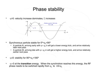
29. Phase stability
• >0: velocity increase dominates, fr increases
• Synchronous particle stable for 0º<s<90º
– A particle N1 arriving early with  s will get a lower energy kick, and arrive relatively
later next pass
– A particle M1 arriving late with  s will get a higher energy kick, and arrive relatively
earlier next pass
• 0: stability for 90º<s<180º
• 0 at the transition energy. When the synchrotron reaches this energy, the RF
phase needs to be switched rapidly from stos

30. Transverse dynamics
Transverse dynamics: degrees of freedom orthogonal to the reference trajectory
ux: the horizontal plane
uy: the vertical plane
Part 4

31. Bending field
• Circular accelerators: deflecting forces are needed
• Circular accelerators: piecewise circular orbits with a defined bending radius

– Straight sections are needed for e.g. particle detectors
– In circular arc sections the magnetic field must provide the desired bending radius:
• For a constant particle energy we need a constant B field  dipole magnets
with homogenous field
• In a synchrotron, the bending radius,1/=eB/p, is kept constant during
acceleration (last section)
B
E F
F
B
v
E
q
F










 )
(
p
eB


1

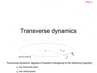
32. The reference trajectory
• An accelerator is designed around a reference trajectory (also called design orbit in
circular accelerators)
• This is the trajectory an ideal particle will follow and consist of
– a straight line where there is no bending field
– arc of circle inside the bending field
• We will in the following talk about transverse deviations from this reference trajectory,
and especially about how to keep these deviations small
Reference trajectory


33. Bending field: dipole magnets
• Dipole magnets provide uniform field in the desired
region
• LHC Dipole magnets: design that allows opposite and
uniform field in both vacuum chambers
• Bonus effect of dipole magnets: geometrical focusing in
the horizontal plane
• 1/: “normalized dipole strength”, strength of the magnet
]
/
[
]
[
3
.
0
]
[
1
1 1
c
GeV
p
T
B
m
p
eB


 



34. Focusing field
• reference trajectory: typically centre of the dipole magnets
• Problem with geometrical focusing: still large oscillations and NO focusing in the
vertical plane  the smallest disturbance (like gravity...) may lead to lost particle
• Desired: a restoring force of the type Fx,y=-kx,y in order to keep the particles
close to the ideal orbit
• A linear field in both planes can be derived from the scalar pot. V(x,y) = gxy
– Equipotential lines at xy=Vconst
– B  magnet iron surface
 Magnet surfaces shaped as hyperbolas gives linear field

35. Focusing field: quadrupoles
• Quadrupole magnets gives linear field in x and y:
Bx = -gy
By = -gx
• However, forces are focusing in one plane and defocusing in the orthogonal
plane:
Fx = -qvgx (focusing)
Fy = qvgy (defocusing)
• Opposite focusing/defocusing is achieved by rotating the quadrupole 90
• Analogy to dipole strength: normalized quadrupole strength:
]
/
[
]
/
[
3
.
0
]
[ 2
c
GeV
p
m
T
g
m
k
p
eg
k 

 
inevitable due to Maxwell

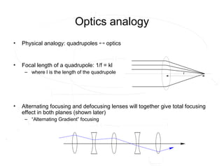
36. Optics analogy
• Physical analogy: quadrupoles  optics
• Focal length of a quadrupole: 1/f = kl
– where l is the length of the quadrupole
• Alternating focusing and defocusing lenses will together give total focusing
effect in both planes (shown later)
– “Alternating Gradient” focusing

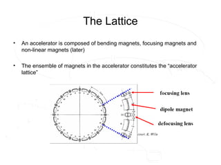
37. The Lattice
• An accelerator is composed of bending magnets, focusing magnets and
non-linear magnets (later)
• The ensemble of magnets in the accelerator constitutes the “accelerator
lattice”

38. Example: lattice components

39. Transverse beam size
RMS beam size:
)
(
)
( s
s rms

 
Beam quality Lattice

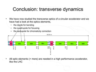
40. Conclusion: transverse dynamics
• We have now studied the transverse optics of a circular accelerator and we
have had a look at the optics elements,
– the dipole for bending
– the quadrupole for focusing
– the sextupole for chromaticity correction
• All optic elements (+ more) are needed in a high performance accelerator,
like the LHC

41. Synchrotron radiation
Part 5

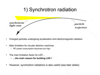
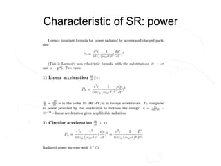
42. 1) Synchrotron radiation
• Charged particles undergoing acceleration emit electromagnetic radiation
• Main limitation for circular electron machines
– RF power consumption becomes too high
• The main limitation factor for LEP...
– ...the main reason for building LHC !
• However, synchrotron radiations is also useful (see later slides)

43. Show RAD2D here
(anim)

44. Characteristic of SR: power

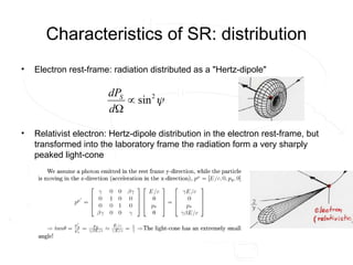
45. Characteristics of SR: distribution
• Electron rest-frame: radiation distributed as a "Hertz-dipole"
• Relativist electron: Hertz-dipole distribution in the electron rest-frame, but
transformed into the laboratory frame the radiation form a very sharply
peaked light-cone

2
sin


d
dPS

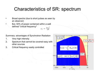
46. • Broad spectra (due to short pulses as seen by
an observer)
• But, 50% of power contained within a well
defined "critical frequency"
Summary: advantages of Synchrotron Radiation
1. Very high intensity
2. Spectrum that cannot be covered easy with
other sources
3. Critical frequency easily controlled
Characteristics of SR: spectrum

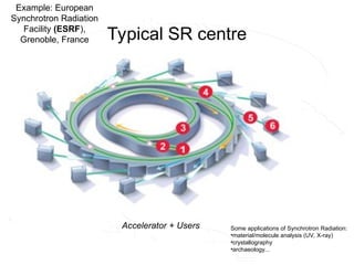
47. Typical SR centre
Accelerator + Users Some applications of Synchrotron Radiation:
•material/molecule analysis (UV, X-ray)
•crystallography
•archaeology...
Example: European
Synchrotron Radiation
Facility (ESRF),
Grenoble, France

48. Case: LHC

49. LHC

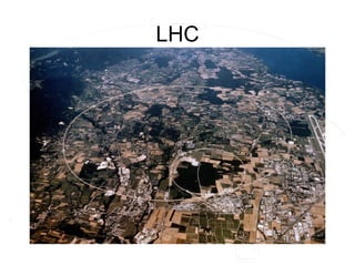
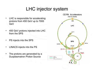
50. LHC injector system
• LHC is responsible for accelerating
protons from 450 GeV up to 7000
GeV
• 450 GeV protons injected into LHC
from the SPS
• PS injects into the SPS
• LINACS injects into the PS
• The protons are generated by a
Duoplasmatron Proton Source

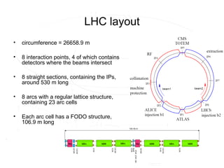
51. LHC layout
• circumference = 26658.9 m
• 8 interaction points, 4 of which contains
detectors where the beams intersect
• 8 straight sections, containing the IPs,
around 530 m long
• 8 arcs with a regular lattice structure,
containing 23 arc cells
• Each arc cell has a FODO structure,
106.9 m long

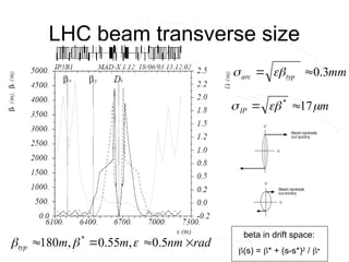
52. LHC beam transverse size
m
IP 

 17
*


mm
typ
arc 3
.
0

 

beta in drift space:
(s) = * + (s-s*)2
/ 
rad
nm
m
m
typ 


 5
.
0
,
55
.
0
,
180 *




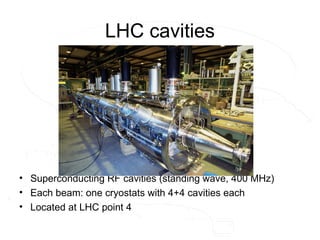
53. LHC cavities
• Superconducting RF cavities (standing wave, 400 MHz)
• Each beam: one cryostats with 4+4 cavities each
• Located at LHC point 4

54. LHC main parameters
at collision energy
Particle type p, Pb
Proton energy Ep at collision 7000 GeV
Peak luminosity (ATLAS,
CMS)
10 x 1034
cm-2
s-1
Circumference C 26 658.9 m
Bending radius  2804.0 m
RF frequency fRF 400.8 MHz
# particles per bunch np 1.15 x 1011
# bunches nb 2808

55. References
• Bibliography:
– K. Wille, The Physics of Particle Accelerators, 2000
– ...and the classic: E. D. Courant and H. S. Snyder, "Theory of the Alternating-
Gradient Synchrotron", 1957
– CAS 1992, Fifth General Accelerator Physics Course, Proceedings, 7-18
September 1992
– LHC Design Report [online]
• Other references
– USPAS resource site, A. Chao, USPAS january 2007
– CAS 2005, Proceedings (in-print), J. Le Duff, B, Holzer et al.
– O. Brüning: CERN student summer lectures
– N. Pichoff: Transverse Beam Dynamics in Accelerators, JUAS January 2004
– U. Amaldi, presentation on Hadron therapy at CERN 2006
– Several figures in this presentation have been borrowed from the above
references, thanks to all!