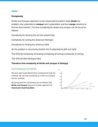
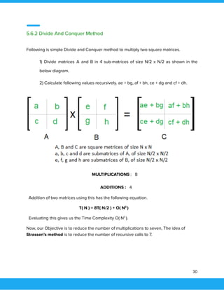
The document discusses the divide and conquer algorithm design paradigm and provides examples of algorithms that use this approach, including binary search, matrix multiplication, and sorting algorithms like merge sort and quicksort. It explains the three main steps of divide and conquer as divide, conquer, and combine. Advantages include solving difficult problems efficiently, enabling parallelization, and optimal memory usage. Disadvantages include issues with recursion, stack size, and choosing base cases. The La Russe method for multiplication is provided as a detailed example that uses doubling and halving to multiply two numbers without the multiplication operator.

1.
ADA - Case Study
Divide & Conquer
Submitted to:
Mr. Neeraj Garg

2.
Submitted By:
Sahil Malik Kushagra Chadha
01214807216, 5C-12 00914807216, 5C-12
Yash Goel Anshuman Raina
01414807216, 5C-12 01396402715, 5C-12
Abhishek Aman Singhal
00596402715, 5C-12 01096402715, 5C-12
1

3.
Contents
1. Introduction 3
2. Understanding Approach 3
Divide/Break 3
Conquer/Solve 4
Merge/Combine 4
3. Advantages of Divide and Conquer Approach 5
Solving difficult problems 5
Algorithm efficiency 5
Parallelism 5
Memory access 5
Round Off control 6
4. Disadvantages of Divide and Conquer Approach 6
Recursion 6
Explicit stack 6
Stack size 7
Choosing the base cases 7
Sharing repeated subproblems 7
5. D&C Algorithms 8
5.1 Binary Search 8
5.2 La Russe Method for Multiplication 11
5.3 Sorting Algorithms 14
5.3.1 Merge Sort 14
5.3.2 Quicksort 17
5.4 Finding Maximum and Minimum of a sequence of Numbers 21
5.5 Closest Pair of points problem 25
5.5.1 Naive method/ Brute force method 25
5.5.2 Divide and Conquer method 27
5.5.3 Comparison of methods 28
5.6 Strassen’s Multiplication Algorithm 29
5.6.1 Naive method/ Brute force method 29
5.6.2 Divide And Conquer Method 30
5.6.3 Strassen's Multiplication Algorithm 31
Conclusion 34
2

4.
1. Introduction
Most of the algorithms are recursive by nature, for solution of any given problem, they try
to break it into smaller parts and solve them individually and at last building solution from
these subsolutions.
In computer science, divide and conquer is an algorithm design paradigm based on
multi-branched recursion. A divide and conquer algorithm works by recursively breaking
down a problem into two or more subproblems of the same or related type, until these
become simple enough to be solved directly. The solutions to the subproblems are then
combined to give a solution to the original problem.
This divide and conquer technique is the basis of efficient algorithms for all kinds of
problems, such as sorting (e.g., quicksort, merge sort), multiplying large numbers (e.g. the
Karatsuba algorithm), finding the closest pair of points, syntactic analysis (e.g., top-down
parsers), and computing the discrete Fourier transform (FFTs).
Understanding and designing divide and conquer algorithms is a complex skill that
requires a good understanding of the nature of the underlying problem to be solved. As
when proving a theorem by induction, it is often necessary to replace the original
problem with a more general or complicated problem in order to initialize the recursion,
and there is no systematic method for finding the proper generalization[clarification
needed]. These divide and conquer complications are seen when optimizing the
calculation of a Fibonacci number with efficient double recursion.
The correctness of a divide and conquer algorithm is usually proved by mathematical
induction, and its computational cost is often determined by solving recurrence relations.
2. Understanding Approach
Broadly, we can understand divide-and-conquer approach in a three-step process.
Divide/Break
This step involves breaking the problem into smaller sub-problems. Sub-problems should
represent a part of the original problem. This step generally takes a recursive approach to divide
3

5.
the problem until no sub-problem is further divisible. At this stage, subproblems become atomic
in nature but still represent some part of the actual problem.
Conquer/Solve
This step receives a lot of smaller sub-problems to be solved. Generally, at this level, the
problems are considered 'solved' on their own.
Merge/Combine
When the smaller subproblems are solved, this stage recursively combines them until they
formulate a solution of the original problem. This algorithmic approach works recursively and
conquer & merge steps works so close that they appear as one.
Examples
The following computer algorithms are based on divide-and-conquer programming approach −
● Merge Sort
● Quick Sort
● Binary Search
● Strassen's Matrix Multiplication
● Closest pair (points)
There are various ways available to solve any computer problem, but the mentioned are a good
example of divide and conquer approach.
4

6.
3. Advantages of Divide and Conquer Approach
- Solving difficult problems
Divide and conquer is a powerful tool for solving conceptually difficult problems: all it
requires is a way of breaking the problem into subproblems, of solving the trivial cases
and of combining sub-problems to the original problem. Similarly, divide and conquer
only requires reducing the problem to a single smaller problem, such as the classic
Tower of Hanoi puzzle, which reduces moving a tower of height n to moving a tower of
height n − 1.
- Algorithm efficiency
The divide-and-conquer paradigm often helps in the discovery of efficient algorithms. It
was the key, for example, to Karatsuba's fast multiplication method, the quicksort and
mergesort algorithms, the Strassen algorithm for matrix multiplication, and fast Fourier
transforms.
In all these examples, the D&C approach led to an improvement in the asymptotic cost
of the solution.
- Parallelism
Divide and conquer algorithms are naturally adapted for execution in multi-processor
machines, especially shared-memory systems where the communication of data
between processors does not need to be planned in advance, because distinct
sub-problems can be executed on different processors.
- Memory access
Divide-and-conquer algorithms naturally tend to make efficient use of memory
caches. The reason is that once a sub-problem is small enough, it and all its
sub-problems can, in principle, be solved within the cache, without accessing the
slower main memory. An algorithm designed to exploit the cache in this way is called
cache-oblivious, because it does not contain the cache size as an explicit
parameter.Moreover, D&C algorithms can be designed for important algorithms (e.g.,
5

7.
sorting, FFTs, and matrix multiplication) to be optimal cache-oblivious algorithms–they
use the cache in a probably optimal way, in an asymptotic sense, regardless of the
cache size. In contrast, the traditional approach to exploiting the cache is blocking, as
in loop nest optimization, where the problem is explicitly divided into chunks of the
appropriate size—this can also use the cache optimally, but only when the algorithm
is tuned for the specific cache size(s) of a particular machine.
- Round Off control
In computations with rounded arithmetic, e.g. with floating point numbers, a
divide-and-conquer algorithm may yield more accurate results than a superficially
equivalent iterative method. For example, one can add N numbers either by a simple
loop that adds each datum to a single variable, or by a D&C algorithm called pairwise
summation that breaks the data set into two halves, recursively computes the sum of
each half, and then adds the two sums. While the second method performs the same
number of additions as the first, and pays the overhead of the recursive calls, it is
usually more accurate.
4. Disadvantages of Divide and Conquer Approach
Like any other approach, D&C too have some difficulties. Most of these are related with
implementation.
- Recursion
Divide-and-conquer algorithms are naturally implemented as recursive procedures. In that case, the
partial sub-problems leading to the one currently being solved are automatically stored in the
procedure call stack. A recursive function is a function that calls itself within its definition.
- Explicit stack
Divide and conquer algorithms can also be implemented by a non-recursive program that stores the
partial sub-problems in some explicit data structure, such as a stack, queue, or priority queue. This
approach allows more freedom in the choice of the sub-problem that is to be solved next, a feature
that is important in some applications — e.g. in breadth-first recursion and the branch and bound
6

8.
method for function optimization. This approach is also the standard solution in programming
languages that do not provide support for recursive procedures.
- Stack size
In recursive implementations of D&C algorithms, one must make sure that there is sufficient memory
allocated for the recursion stack, otherwise the execution may fail because of stack overflow.
Fortunately, D&C algorithms that are time-efficient often have relatively small recursion depth. For
example, the quicksort algorithm can be implemented so that it never requires more than log2 n
nested recursive calls to sort n items.
- Choosing the base cases
In any recursive algorithm, there is considerable freedom in the choice of the base cases, the small
subproblems that are solved directly in order to terminate the recursion.
Choosing the smallest or simplest possible base cases is more elegant and usually leads to simpler
programs, because there are fewer cases to consider and they are easier to solve.
On the other hand, efficiency often improves if the recursion is stopped at relatively large base cases,
and these are solved non-recursively, resulting in a hybrid algorithm.
The generalized version of this idea is known as recursion "unrolling" or "coarsening" and various
techniques have been proposed for automating the procedure of enlarging the base case.
- Sharing repeated subproblems
For some problems, the branched recursion may end up evaluating the same sub-problem
many times over. In such cases it may be worth identifying and saving the solutions to these
overlapping subproblems, a technique commonly known as memoization. Followed to the
limit, it leads to bottom-up divide-and-conquer algorithms such as dynamic programming and
chart parsing.
7

9.
5. D&C Algorithms
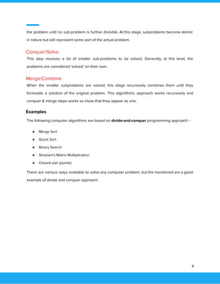
5.1 Binary Search
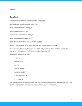
Binary search is a fast search algorithm with run-time complexity of Ο(log n). This search
algorithm works on the principle of divide and conquer. For this algorithm to work properly, the
data collection should be in the sorted form
Algorithm
if(l=i) then
{
if(x=a[i]) return i;
else return 0;
}
else
{
//reduce to smaller subproblems
mid=(mid+1)/2;
if(x=a[mid]) then return mid;
else if(x<a[mid]) then return BinSearch(a,i,mid-1,x)
else return BinSearch(a,mid+1,l,x)
}
8

10.
Complexity
Time complexity of binary search algorithm is O(log2(N)).
At a glance the complexity table is like this -
Worst case performance : O(log2 n)
Best case performance : O(1)
Average case performance: O(log2 n)
Worst case space complexity: O(1)
But that is not the fact, the fact is why it is log2(N) ?
Here is a mathematical proof which describe why the complexity is log2(N).
The question is, how many times can you divide N by 2 until you have 1? This is essentially
saying, do a binary search (half the elements) until you found it.
In a formula this would be this:
1 = N / 2x
multiply by 2x:
2x = N
now do the log2:
log2(2x) = log2 N
x * log2(2) = log2 N
x * 1 = log2 N
This means you can divide log N times until you have everything divided. Which means you have
to divide log N ("do the binary search step") until you found your element.
9

11.
Example
# Python Program for recursive binary search.
# Returns index of x in arr if present, else -1.
def binarySearch (arr, l, r, x):
# Check base case
if r >= l:
mid = l + (r - l)/2
# If element is present at the middle itself
if arr[mid] == x:
return mid
# If element is smaller than mid, then it can only
# be present in left subarray
elif arr[mid] > x:
return binarySearch(arr, l, mid-1, x)
# Else the element can only be present in right subarray
else:
return binarySearch(arr, mid+1, r, x)
else:
# Element is not present in the array
return -1
# Test array
arr = [ 2, 3, 4, 10, 40 ]
x = 10
# Function call
result = binarySearch(arr, 0, len(arr)-1, x)
if result != -1:
print "Element is present at index %d" % result
else:
print "Element is not present in array"
Output
10

12.
5.2 La Russe Method for Multiplication
La Russe Method follows a Divide and Conquer Approach for multiplication of two 2 or
more digit numbers. It works on following underlying principle:
Let a and b be two integers of minimum 2 digit length. The value of a*b is same as
(a*2)*(b/2) if b is even, otherwise the value is same as ((a*2)*(b/2) + a). In the while loop,
we keep multiplying ‘a’ with 2 and keep dividing ‘b’ by 2. If ‘b’ becomes odd in loop, we
add ‘a’ to ‘res’. When value of ‘b’ becomes 1, the value of ‘res’ + ‘a’, gives us the result.
Note: that when ‘b’ is a power of 2, the ‘res’ would remain 0 and ‘a’ would have the
multiplication.
So, in simple terms, Given two integers, write a function to multiply them without using
multiplication operator.One interesting method is the Russian peasant algorithm. The
idea is to double the first number and halve the second number repeatedly till the
second number doesn’t become 1. In the process, whenever the second number become
odd, we add the first number to result (result is initialized as 0)
Algorithm:
1. Let the two given numbers be 'a' and 'b'
2. Initialize result 'res' as 0.
3. Do following while 'b' is greater than 0
a. If 'b' is odd, add 'a' to 'res'
b. Double 'a' and halve 'b'
4. return res
Rules:
● Write each number at the head of a column.
● Double the number in the first column, and halve the number in the second column
● If the number in the second column is odd, divide it by two and drop the remainder.
● If the number in the second column is even, cross out that entire row.
● Keep doubling, halving, and crossing out until the number in the second column is 1.
● Add up the remaining numbers in the first column. The total is the product of your original
number.
11

13.
Multiply 57 by 86 as an example:
Write each number at the head of a column.
57 86
Double the number in the first column, and halve the number in the second column.
57 86
114 43
If the number in the second column is even, cross out that entire row.
57 86
114 43
Keep doubling, halving, and crossing out until the number in the second column is 1.
57 86
114 43
228 21
456 10
912 5
1824 2
3648 1
Add up the remaining numbers in the first column.
57 86
114 43
228 21
456 10
912 5
1824 2
+ 3648 1
4902
12

14.
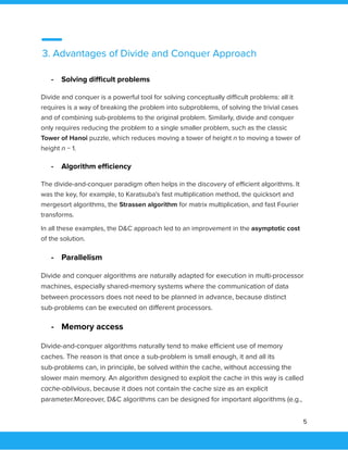
Source code:
import java.io.*;
class laRusseMultAlgo
{
static int russianPeasant(int a, int b)
{
int res = 0;
while (b > 0)
{
if ((b & 1) != 0)
res = res + a;
a = a << 1;
b = b >> 1;
}
return res;
}
public static void main (String[] args)
{
System.out.println(russianPeasant(18, 1));
System.out.println(russianPeasant(20, 12));
}
}
Output:
18
240
13

15.
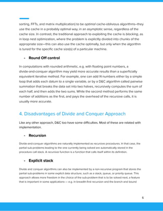
5.3 Sorting Algorithms
There are a few algorithms for sorting which follow Divide & Conquer Approach. We will
study two major ones, Merge Sort and Quicksort.
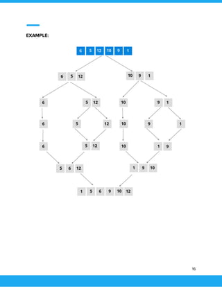
5.3.1 Merge Sort
Merge Sort is a Divide and Conquer algorithm. It divides input array in two halves, calls
itself for the two halves and then merges the two sorted halves. The merge() function is
used for merging two halves. The merge(arr, l, m, r) is key process that assumes that
arr[l..m] and arr[m+1..r] are sorted and merges the two sorted sub-arrays into one.
Merge Sort Approach
•Divide
–Divide the n-element sequence to be sorted into two subsequences of n/2 elements
each
•Conquer
–Sort the subsequences recursively using merge sort
–When the size of the sequences is 1 there is nothing more to do
•Combine
–Merge the two sorted subsequences
Algorithm
MERGE-SORT(A, p, r)
if p < r Check for base case
then q ← [(p + r)/2] Divide
MERGE-SORT(A, p, q) Conquer
MERGE-SORT(A, q + 1, r) Conquer
MERGE(A, p, q, r) Combine
14

16.
MERGE(A, p, q, r)
➔ Create copies of the subarrays L ← A[p..q] and M ← A[q+1..r].
➔ Create three pointers i,j and k
◆ i maintains current index of L, starting at 1
◆ j maintains current index of M, starting at 1
◆ k maintains current index of A[p..q], starting at p
➔ Until we reach the end of either L or M, pick the larger among the elements from L
and M and place them in the correct position at A[p..q]
➔ When we run out of elements in either L or M, pick up the remaining elements and
put in A[p..q]
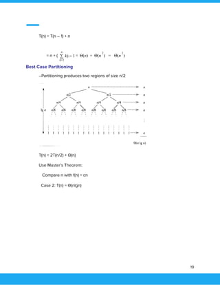
MERGE-SORT Running Time
•Divide:
–compute q as the average of p and r: D(n) = θ (1)
•Conquer:
–recursively solve 2 subproblems, each of size n/2 => 2T (n/2)
•Combine:
–MERGE on an n-element subarray takes θ (n) time C(n) = θ (n)
θ (1) if n =1
T(n) =
2T(n/2) + θ (n) if n > 1
Use Master’s Theorem:
Compare n with f(n) = cn
Case 2: T(n) = Θ(n log n)
15

17.
EXAMPLE:
16

18.
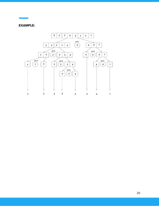
5.3.2 Quicksort
QuickSort is a Divide and Conquer algorithm. It picks an element as pivot and partitions
the given array around the picked pivot. There are many different versions of quickSort
that pick pivot in different ways.
Quicksort Approach
•Divide
–Partition the array A into 2 subarrays A[p..q] and A[q+1..r], such that each element
of A[p..q] is smaller than or equal to each element in A[q+1..r]
–Need to find index q to partition the array
•Conquer
–Recursively sort A[p..q] and A[q+1..r] using Quicksort
•Combine
–Trivial: the arrays are sorted in place
–No additional work is required to combine them
–The entire array is now sorted.
Algorithm
QUICKSORT(A, p, r)
if p < r
then q ← PARTITION(A, p, r)
QUICKSORT (A, p, q)
QUICKSORT (A, q+1, r)
17

19.
PARTITION (A, p, r)
x ← A[p]
i ← p – 1
j ← r + 1
while TRUE
do repeat j ← j – 1
until A[j] ≤ x
do repeat i ← i + 1
until A[i] ≥ x
if i < j
then exchange A[i] ↔ A[j]
else return j
QUICK-SORT Running Time
For Worst-case partitioning
–One region has one element and the other has n – 1 elements
–Maximally unbalanced
T(n) = T(1) + T(n – 1) + n,
T(1) = Q(1)
18

20.
T(n) = T(n – 1) + n
= n + ( =)∑
n
k=1
k − 1 (n) Θ(n ) Θ(n )Θ +
2
=
2
Best Case Partitioning
–Partitioning produces two regions of size n/2
T(n) = 2T(n/2) + Θ(n)
Use Master’s Theorem:
Compare n with f(n) = cn
Case 2: T(n) = Θ(nlgn)
19

21.
EXAMPLE:
20

22.
5.4 Finding Maximum and Minimum of a sequence of Numbers
This method is also known as Tournament method.
This method is used, as the name suggests, for finding the maximum and the minimum
numbers present in any given sequence of numbers. This works on negative as well as
on decimal numbers, which makes it applicable on all types of numeric data types.
Algorithm
Let MaxMin be any function which takes in an Array of numbers and size of array, and it
returns the pair of numbers which are maximum and minimum in array
MaxMin(array, array_size)
if array_size = 1
return element as both max and min
else if arry_size = 2
one comparison to determine max and min
return that pair
else array_size > 2
recur for max and min of left half
recur for max and min of right half
one comparison determines true max of the two candidates
one comparison determines true min of the two candidates
return the pair of max and min
21

23.
Complexity
Consider n=8 elements in an array {1,4,5,8,3,2,7,9}
Let’s make a tournament bracket for them, where at each stage the winner is the
minimum element between the two.
As we can see, number of comparisons
being done = n-1 = 7
Similarly, to find the maximum element you again will need n-1 comparisons!
So total no of comparisons to find min and max=2(n-1)
There is one optimisation to it !!
The last level in the tree is making n/2 comparisons(4 in this case) and these are
being repeated while finding the minimum and maximum!
So doing the last level comparisons only once, we do n/2 comparisons less
Hence 2(n-1) - n/2 = 2n-2 - n/2 = (3n/2) - 2.
And when compared to normal iterative method of using loops, loop will run n times and
there will be two comparisons, which gives 2n.
So Tournament Method is faster.
22

24.
Example
Consider following example of Tournament Method in Java:
class pair{
public int max, min;
}
public class HelloWorld
{
public static void main(String[] args)
{
float[] arr = {-34, 43,45,2,46};
pair p = getMinMax(arr, 0, arr.length-1);
System.out.println(p.max+" "+p.min);
}
public static pair getMinMax(float[] arr, int start, int end){
pair minmax =new pair(), mml=new pair(), mmr=new pair();
int mid;
if (start == end){
minmax.max = arr[start];
minmax.min = arr[start];
return minmax;
}
if (end == start+ 1){
if (arr[start] > arr[end]) {
minmax.max = arr[start];
minmax.min = arr[end];
}
else{
minmax.max = arr[end];
minmax.min = arr[start];
}
return minmax;
}
mid = (start + end)/2;
mml = getMinMax(arr, start, mid);
23

25.
mmr = getMinMax(arr, mid+1, end);
if (mml.min < mmr.min)
minmax.min = mml.min;
else
minmax.min = mmr.min;
if (mml.max > mmr.max)
minmax.max = mml.max;
else
minmax.max = mmr.max;
return minmax;
}
}
Output:
24

26.
5.5 Closest Pair of points problem
Given a finite set of n points in the plane, the goal is to find
the closest pair, that is, the distance between the two closest
points. Formally, we want to find a distance δ such that there
exists a pair of points (ai , aj) at distance δ of each other, and
such that any other two points are separated by a distance
greater than or equal to δ. The above stated can be achieved
by two approaches-
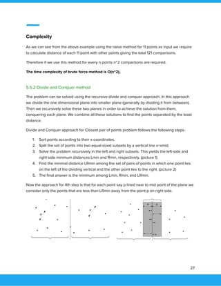
5.5.1 Naive method/ Brute force method
Given the set of points we iterate over each and every point in the plain calculating the
distances between them and storing them. Then the minimum distance is chosen which
gets us the solution to the problem.
Algorithm
minDist = infinity
for i = 1 to length(P) - 1
for j = i + 1 to length(P)
let p = P[i], q = P[j]
if dist(p, q) < minDist:
minDist = dist(p, q)
closestPair = (p, q)
return closestPair
25

27.
Example
Consider the following python code demonstrating the naive method-
import math
def calculateDistance(x1, y1, x2, y2):
dist = math.sqrt((x2 - x1) ** 2 + (y2 - y1) ** 2)
return dist
def closest(x,y):
result=[0,0]
min=999999
for i in range(len(x)):
for j in range(len(x)):
if i==j:
pass
else:
dist=calculateDistance(x[i],y[i],x[j],y[j]);
if dist<=min:
min=dist;
result[0]=i
result[1]=j
print("Closest distance is between point "+str(result[0]+1)+" and "+str(result[1]+1)+"
and distance is-"+str(min))
x=[5,-6,8,9,-10,0,20,6,7,8,9]
y=[0,-6,7,2,-1,5,-3,6,3,8,-9]
closest(x,y)
26

28.
Complexity
As we can see from the above example using the naive method for 11 points as input we require
to calculate distance of each 11 point with other points giving the total 121 comparisons.
Therefore if we use this method for every n points n^2 comparisons are required.
The time complexity of brute force method is O(n^2),
5.5.2 Divide and Conquer method
The problem can be solved using the recursive divide and conquer approach. In this approach
we divide the one dimensional plane into smaller plane (generally by dividing it from between).
Then we recursively solve these two planes in order to achieve the solution from them,
conquering each plane. We combine all these solutions to find the points separated by the least
distance.
Divide and Conquer approach for Closest pair of points problem follows the following steps-
1. Sort points according to their x-coordinates.
2. Split the set of points into two equal-sized subsets by a vertical line x=xmid.
3. Solve the problem recursively in the left and right subsets. This yields the left-side and
right-side minimum distances Lmin and Rmin, respectively. (picture 1)
4. Find the minimal distance LRmin among the set of pairs of points in which one point lies
on the left of the dividing vertical and the other point lies to the right. (picture 2)
5. The final answer is the minimum among Lmin, Rmin, and LRmin.
Now the approach for 4th step is that for each point say p lined near to mid point of the plane we
consider only the points that are less than LRmin away from the point p on right side.
27

29.
Complexity
Divide and Conquer approach to the closest point problem helps divide the
problem into subproblems conquer each subproblem and then merge solutions to
find the final solution. The time complexity for divide and conquer can be found as
follows-
Complexity for dividing the set into subset=O(n)
Complexity for sorting the distances=O(nlogn)
Complexity for finding the distances=O(n)
As the problem is recursively divided into 2 subproblems (left and right)
T(n)=2T(n/2)+complexity of dividing+complexity of sorting+complexity of solving
T(n)=2T(n/2)+O(n)+O(nlogn)+O(n)
Therefore time complexity of divide and conquer is O(nlogn)
5.5.3 Comparison of methods
We were able to get defined time complexity for both the
methods. We use that complexity as a metric to compare
the two methods.
By seeing both the complexities we can deduce that
Divide and Conquer approach is better approach for
closest pair of point problem.
28

30.
5.6 Strassen’s Multiplication Algorithm
Problem Statement
Considering two matrices X and Y, we need to calculate the resultant product Matrix Z of
X and Y.
5.6.1 Naive method/ Brute force method
First, we will discuss naïve method and its complexity. Here, we are calculating Z = X × Y.
Using Naïve method, two matrices (X and Y) can be multiplied if the order of these
matrices are p × q and q × r. The resultant product matrix Z will have the order of p × r.
Algorithm : ( Brute Force )
Analysis:
In the above Algo, we see that i runs from 1 to p . Then j runs from 1 to q . Inside the
nested loops, the last loop runs from 1 to r . Thus the complexity for such a looping
Algorithm is O(n3
).
Naive Method can be quite lengthy, thus we try to reduce its size by using Divide And
Conquer.
29

31.
5.6.2 Divide And Conquer Method
Following is simple Divide and Conquer method to multiply two square matrices.
1) Divide matrices A and B in 4 sub-matrices of size N/2 x N/2 as shown in the
below diagram.
2) Calculate following values recursively. ae + bg, af + bh, ce + dg and cf + dh.
MULTIPLICATIONS : 8
ADDITIONS : 4
Addition of two matrices using this has the following equation.
T( N ) = 8T( N/2 ) + O( N2
)
Evaluating this gives us the Time Complexity O( N3
).
Now, our Objective is to reduce the number of multiplications to seven, The idea of
Strassen’s method is to reduce the number of recursive calls to 7.
30

32.
5.6.3 Strassen's Multiplication Algorithm
As said earlier, Strassen’s Algorithm is similar to DIvide and Conquer Algorithm.
Strassen’s method is similar to above simple divide and conquer method in the sense
that this method also divide matrices to sub-matrices of size N/2 x N/2 .Only here
emphasis is on reducing the time complexity so as to gain the resultant matrix in the best
possible time complexity.
He defined P1, P2, P3, P4, P5, P6 and P7 as defined on the image below.
Complexity
As I mentioned above the Strassen’s algorithm is slightly faster than the general matrix
multiplication algorithm. The general algorithm’s time complexity is O(n^3), while the
Strassen’s algorithm is O( n^2.80 ) = O( n log27 ) .
31

33.
You can see on the chart below how slightly faster is this even for large n
Fig. Comparison of time complexities between Strassen and Naive Algorithm.
Application
Although this algorithm seems to be more close to pure mathematics than to computer
practically everywhere we use NxN arrays we can benefit from matrix multiplication.
In the other hand the algorithm of Strassen is not much faster than the general n^3 matrix
multiplication algorithm. That’s very important because for small n (usually n < 45) the
general algorithm is practically a better choice. However as you can see from the chart
above for n > 100 the difference can be very big.
32

34.
Time Complexity of Strassen’s Method
3.6.4 Application In Real World
Generally Strassen’s Method is not preferred for practical applications for following
reasons :
● The constants used in Strassen’s method are high and for a typical application
Naive method works better.
● For Sparse matrices, there are better methods especially designed for them.
The submatrices in recursion take extra space.
● Because of the limited precision of computer arithmetic on noninteger values,
larger errors accumulate in Strassen’s algorithm than in Naive Method
33

35.
Conclusion
The Divide-and-Conquer paradigm can be described in this way:
Given an instance of the problem to be solved, split this into several, smaller,
sub-instances (of the same problem) independently solve each of the sub-instances and
then combine the sub-instance solutions so as to yield a solution for the original instance.
It gives very efficient solutions. It is the choice when the following is true:
1. the problem can be described recursively - in terms of smaller instances of
the same problem.
2. the problem-solving process can be described recursively, i.e. we can
combine the solutions of the smaller instances to obtain the solution of the
original problem
Note that we assume that the problem is split in at least two parts of equal size, not
simply decreased by a constant factor.
34