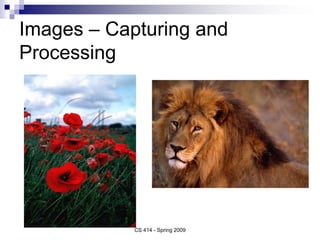
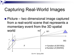
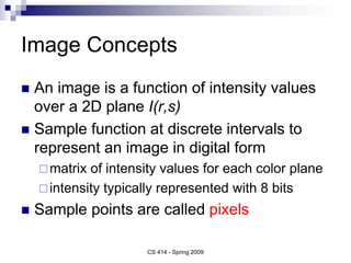
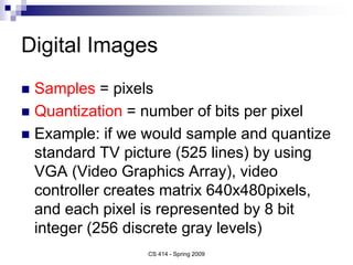
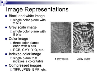
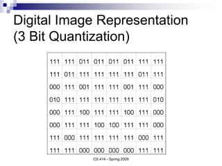
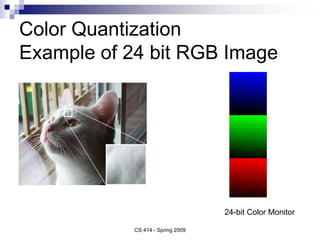
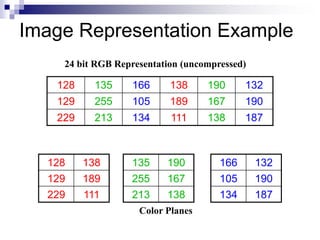
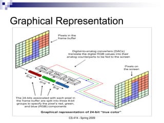
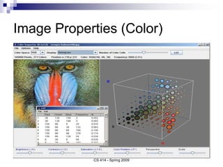
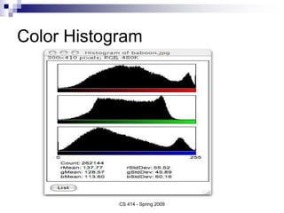
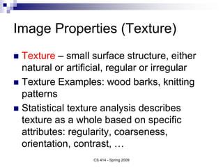
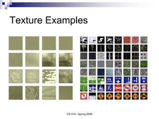
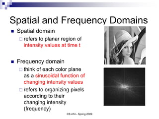
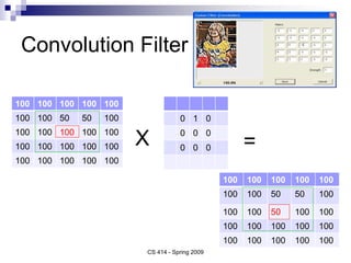
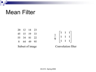
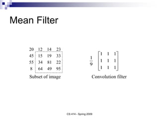
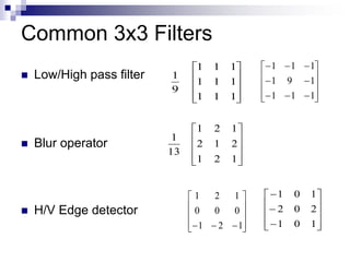
CS 414 - Spring 2009
CS 414 – Multimedia Systems Design
Lecture 4 – Digital Image
Representation
Klara Nahrstedt
Spring 2009
CS 414 - Spring 2009
Administrative
 Group Directories will be established
hopefully today (or latest by Friday)
 MP1 will be out on 1/28 (today)
 Start by reading the MP1 and organizing
yourself as a group this week, start to read
documentation, search for audio and video
files.
Images – Capturing and
Processing
CS 414 - Spring 2009
Capturing Real-World Images
 Picture – two dimensional image captured
from a real-world scene that represents a
momentary event from the 3D spatial
world
CS 414 - Spring 2009
W3
W1
W2
r
s
F r= function of (W1/W3);
s=function of (W2/W3)
Image Concepts
 An image is a function of intensity values
over a 2D plane I(r,s)
 Sample function at discrete intervals to
represent an image in digital form
matrix of intensity values for each color plane
intensity typically represented with 8 bits
 Sample points are called pixels
CS 414 - Spring 2009
Digital Images
 Samples = pixels
 Quantization = number of bits per pixel
 Example: if we would sample and quantize
standard TV picture (525 lines) by using
VGA (Video Graphics Array), video
controller creates matrix 640x480pixels,
and each pixel is represented by 8 bit
integer (256 discrete gray levels)
CS 414 - Spring 2009
Image Representations
 Black and white image
 single color plane with
2 bits
 Grey scale image
 single color plane with
8 bits
 Color image
 three color planes
each with 8 bits
 RGB, CMY, YIQ, etc.
 Indexed color image
 single plane that
indexes a color table
 Compressed images
 TIFF, JPEG, BMP, etc.
2gray levels
4 gray levels
Digital Image Representation
(3 Bit Quantization)
CS 414 - Spring 2009
Color Quantization
Example of 24 bit RGB Image
CS 414 - Spring 2009
24-bit Color Monitor
Image Representation Example
128 135 166 138 190 132
129 255 105 189 167 190
229 213 134 111 138 187
135 190
255 167
213 138
128 138
129 189
229 111
166 132
105 190
134 187
24 bit RGB Representation (uncompressed)
Color Planes
Graphical Representation
CS 414 - Spring 2009
Image Properties (Color)
CS 414 - Spring 2009
Color Histogram
CS 414 - Spring 2009
Image Properties (Texture)
 Texture – small surface structure, either
natural or artificial, regular or irregular
 Texture Examples: wood barks, knitting
patterns
 Statistical texture analysis describes
texture as a whole based on specific
attributes: regularity, coarseness,
orientation, contrast, …
CS 414 - Spring 2009
Texture Examples
CS 414 - Spring 2009
Spatial and Frequency Domains
 Spatial domain
 refers to planar region of
intensity values at time t
 Frequency domain
 think of each color plane
as a sinusoidal function of
changing intensity values
 refers to organizing pixels
according to their
changing intensity
(frequency)
CS 414 - Spring 2009
Image Processing Function: 1. Filtering
 Filter an image by replacing each pixel in the
source with a weighted sum of its neighbors
 Define the filter using a convolution mask, also
referred to as a kernel
 non-zero values in small neighborhood, typically
centered around a central pixel
 generally have odd number of rows/columns
CS 414 - Spring 2009
Convolution Filter
CS 414 - Spring 2009
100 100 100 100 100
100 100 50 50 100
100 100 100 100 100
100 100 100 100 100
100 100 100 100 100
0 1 0
0 0 0
0 0 0
100 100 100 100 100
100 100 50 50 100
100 100 50 100 100
100 100 100 100 100
100 100 100 100 100
X =
Mean Filter
Convolution filter
Subset of image
95
49
64
8
22
81
34
55
33
19
15
45
23
14
12
20










1
1
1
1
1
1
1
1
1
9
1
CS 414 - Spring 2009
Mean Filter
Convolution filter
Subset of image
95
49
64
8
22
81
34
55
33
19
15
45
23
14
12
20










1
1
1
1
1
1
1
1
1
9
1
CS 414 - Spring 2009
Common 3x3 Filters
 Low/High pass filter
 Blur operator
 H/V Edge detector










1
2
1
2
1
2
1
2
1
13
1


















1
1
1
1
9
1
1
1
1












 1
2
1
0
0
0
1
2
1













1
0
1
2
0
2
1
0
1










1
1
1
1
1
1
1
1
1
9
1
Example
CS 414 - Spring 2009
Image Function: 2. Edge Detection
 Identify areas of strong
intensity contrast
 filter useless data; preserve
important properties
 Fundamental technique
 e.g., use gestures as input
 identify shapes, match to
templates, invoke commands
Edge Detection
CS 414 - Spring 2009
Simple Edge Detection
 Example: Let assume single line of pixels
 Calculate 1st derivative (gradient) of the
intensity of the original data
 Using gradient, we can find peak pixels in image
 I(x) represents intensity of pixel x and
 I’(x) represents gradient (in 1D),
 Then the gradient can be calculated by convolving the
original data with a mask (-1/2 0 +1/2)
 I’(x) = -1/2 *I(x-1) + 0*I(x) + ½*I(x+1)
CS 414 - Spring 2008
5 7 6 4 152 148 149
Basic Method of Edge Detection
 Step 1: filter noise using mean filter
 Step 2: compute spatial gradient
 Step 3: mark points > threshold as edges
CS 414 - Spring 2009
Mark Edge Points
 Given gradient at each
pixel and threshold
 mark pixels where
gradient > threshold as
edges
CS 414 - Spring 2009
Compute Edge Direction
 Calculation of Rate of Change in
Intensity Gradient
 Use 2nd derivative
 Example: (5 7 6 4 152 148 149)
 Use convolution mask (+1 -2 +1)
 I’’(x) = 1*I(x-1) -2*I(x) + 1*I(x+1)
 Peak detection in 2nd derivate
is a method for line detection.
CS 414 - Spring 2009
Summary
 Other Important Image Processing Functions
 Image segmentation
 Image recognition
 Formatting
 Conditioning
 Marking
 Grouping
 Extraction
 Matching
 Image synthesis
CS 414 - Spring 2009

Digital Image Representation.ppt

  • 1.
    CS 414 -Spring 2009 CS 414 – Multimedia Systems Design Lecture 4 – Digital Image Representation Klara Nahrstedt Spring 2009
  • 2.
    CS 414 -Spring 2009 Administrative  Group Directories will be established hopefully today (or latest by Friday)  MP1 will be out on 1/28 (today)  Start by reading the MP1 and organizing yourself as a group this week, start to read documentation, search for audio and video files.
  • 3.
    Images – Capturingand Processing CS 414 - Spring 2009
  • 4.
    Capturing Real-World Images Picture – two dimensional image captured from a real-world scene that represents a momentary event from the 3D spatial world CS 414 - Spring 2009 W3 W1 W2 r s F r= function of (W1/W3); s=function of (W2/W3)
  • 5.
    Image Concepts  Animage is a function of intensity values over a 2D plane I(r,s)  Sample function at discrete intervals to represent an image in digital form matrix of intensity values for each color plane intensity typically represented with 8 bits  Sample points are called pixels CS 414 - Spring 2009
  • 6.
    Digital Images  Samples= pixels  Quantization = number of bits per pixel  Example: if we would sample and quantize standard TV picture (525 lines) by using VGA (Video Graphics Array), video controller creates matrix 640x480pixels, and each pixel is represented by 8 bit integer (256 discrete gray levels) CS 414 - Spring 2009
  • 7.
    Image Representations  Blackand white image  single color plane with 2 bits  Grey scale image  single color plane with 8 bits  Color image  three color planes each with 8 bits  RGB, CMY, YIQ, etc.  Indexed color image  single plane that indexes a color table  Compressed images  TIFF, JPEG, BMP, etc. 2gray levels 4 gray levels
  • 8.
    Digital Image Representation (3Bit Quantization) CS 414 - Spring 2009
  • 9.
    Color Quantization Example of24 bit RGB Image CS 414 - Spring 2009 24-bit Color Monitor
  • 10.
    Image Representation Example 128135 166 138 190 132 129 255 105 189 167 190 229 213 134 111 138 187 135 190 255 167 213 138 128 138 129 189 229 111 166 132 105 190 134 187 24 bit RGB Representation (uncompressed) Color Planes
  • 11.
  • 12.
    Image Properties (Color) CS414 - Spring 2009
  • 13.
  • 14.
    Image Properties (Texture) Texture – small surface structure, either natural or artificial, regular or irregular  Texture Examples: wood barks, knitting patterns  Statistical texture analysis describes texture as a whole based on specific attributes: regularity, coarseness, orientation, contrast, … CS 414 - Spring 2009
  • 15.
  • 16.
    Spatial and FrequencyDomains  Spatial domain  refers to planar region of intensity values at time t  Frequency domain  think of each color plane as a sinusoidal function of changing intensity values  refers to organizing pixels according to their changing intensity (frequency) CS 414 - Spring 2009
  • 17.
    Image Processing Function:1. Filtering  Filter an image by replacing each pixel in the source with a weighted sum of its neighbors  Define the filter using a convolution mask, also referred to as a kernel  non-zero values in small neighborhood, typically centered around a central pixel  generally have odd number of rows/columns CS 414 - Spring 2009
  • 18.
    Convolution Filter CS 414- Spring 2009 100 100 100 100 100 100 100 50 50 100 100 100 100 100 100 100 100 100 100 100 100 100 100 100 100 0 1 0 0 0 0 0 0 0 100 100 100 100 100 100 100 50 50 100 100 100 50 100 100 100 100 100 100 100 100 100 100 100 100 X =
  • 19.
    Mean Filter Convolution filter Subsetof image 95 49 64 8 22 81 34 55 33 19 15 45 23 14 12 20           1 1 1 1 1 1 1 1 1 9 1 CS 414 - Spring 2009
  • 20.
    Mean Filter Convolution filter Subsetof image 95 49 64 8 22 81 34 55 33 19 15 45 23 14 12 20           1 1 1 1 1 1 1 1 1 9 1 CS 414 - Spring 2009
  • 21.
    Common 3x3 Filters Low/High pass filter  Blur operator  H/V Edge detector           1 2 1 2 1 2 1 2 1 13 1                   1 1 1 1 9 1 1 1 1              1 2 1 0 0 0 1 2 1              1 0 1 2 0 2 1 0 1           1 1 1 1 1 1 1 1 1 9 1
  • 22.
    Example CS 414 -Spring 2009
  • 23.
    Image Function: 2.Edge Detection  Identify areas of strong intensity contrast  filter useless data; preserve important properties  Fundamental technique  e.g., use gestures as input  identify shapes, match to templates, invoke commands
  • 24.
    Edge Detection CS 414- Spring 2009
  • 25.
    Simple Edge Detection Example: Let assume single line of pixels  Calculate 1st derivative (gradient) of the intensity of the original data  Using gradient, we can find peak pixels in image  I(x) represents intensity of pixel x and  I’(x) represents gradient (in 1D),  Then the gradient can be calculated by convolving the original data with a mask (-1/2 0 +1/2)  I’(x) = -1/2 *I(x-1) + 0*I(x) + ½*I(x+1) CS 414 - Spring 2008 5 7 6 4 152 148 149
  • 26.
    Basic Method ofEdge Detection  Step 1: filter noise using mean filter  Step 2: compute spatial gradient  Step 3: mark points > threshold as edges CS 414 - Spring 2009
  • 27.
    Mark Edge Points Given gradient at each pixel and threshold  mark pixels where gradient > threshold as edges CS 414 - Spring 2009
  • 28.
    Compute Edge Direction Calculation of Rate of Change in Intensity Gradient  Use 2nd derivative  Example: (5 7 6 4 152 148 149)  Use convolution mask (+1 -2 +1)  I’’(x) = 1*I(x-1) -2*I(x) + 1*I(x+1)  Peak detection in 2nd derivate is a method for line detection. CS 414 - Spring 2009
  • 29.
    Summary  Other ImportantImage Processing Functions  Image segmentation  Image recognition  Formatting  Conditioning  Marking  Grouping  Extraction  Matching  Image synthesis CS 414 - Spring 2009