This document is a tutorial for using Theano, presented at the Moscow Data Fest, which covers basic functionalities, shared variables, logistic regression, and support vector machines (SVM). It includes code snippets that demonstrate how to implement these concepts, visualize results, and optimize models using gradient descent. Additionally, it provides links to access the tutorial code and the event details.

1. DataFest Theano tutorial
September 20, 2015
1 Introduction
This is a basic theano tutorial, presented at the Moscow Data Fest: http://www.meetup.com/Moscow-Data-
Fest/events/224856462/.
You can find the code here: https://github.com/dudevil/datafest-theano-tutorial/.
1.1 Baby steps
In [1]: import numpy as np
import theano
import theano.tensor as T
%pylab inline
figsize(8, 6)
Populating the interactive namespace from numpy and matplotlib
In [18]: # declare theano variable
a = theano.tensor.lscalar()
#a = theano.tensor.vector()
expression = 1 + 2 * a + a ** 2
f = theano.function(
[a],
expression)
In [7]: #f(0)
result = f(np.arange(-10, 10))
result
Out[7]: array([ 81., 64., 49., 36., 25., 16., 9., 4., 1.,
0., 1., 4., 9., 16., 25., 36., 49., 64.,
81., 100.])
In [8]: plot(np.arange(-10, 10), result, c=’m’, linewidth=2.)
grid()
1

2. In [9]: # shared variables represent internal state
state = theano.shared(0)
i = T.iscalar(’i’)
accumulator = theano.function([i],
state,
updates=[(state, state+i)])
In [14]: accumulator(5)
Out[14]: array(20)
In [15]: state.set_value(-15)
print state.get_value()
-15
In [19]: state.set_value(0)
f = theano.function(
[i],
expression,
updates=[(state, state+i)],
givens={
a : state
}
)
2

3. In [25]: f(1)
Out[25]: array(36)
1.2 Data
In [26]: x1 = np.linspace(-1, 1, 100)
x2 = 1.5 - x1 ** 2 + np.random.normal(scale=0.2, size=100)
x3 = np.random.normal(scale=0.3, size=100)
x4 = np.random.normal(scale=0.3, size=100)
permutation = np.random.permutation(np.arange(200))
x = np.hstack((
np.vstack((x1, x2)),
np.vstack((x3, x4)))).T[permutation]
y = np.concatenate((
np.zeros_like(x1),
np.ones_like(x3)))[permutation]
# needed for pictures later
xx, yy = np.mgrid[-2:2:.01, -2:2:.01]
grid_arr = np.c_[xx.ravel(), yy.ravel()]
def plot_decision(predicts):
probas = predicts.reshape(xx.shape)
contour = contourf(xx, yy, probas, 25, cmap="RdBu", vmin=0, vmax=1)
colorbar(contour)
scatter(x[:,0], x[:, 1], c=y, s=50,
cmap="RdBu", vmin=-.2, vmax=1.2,
edgecolor="white", linewidth=1)
title("Some cool decision boundary")
grid()
In [27]: scatter(x[:,0], x[:, 1], c=y, s=75,
cmap="RdBu", vmin=-.2, vmax=1.2,
edgecolor="white", linewidth=1)
title("Toy data")
grid()
3

4. 1.3 Logistic regression
In [29]: # allocate variables
W = theano.shared(
value=numpy.zeros((2, 1),dtype=theano.config.floatX),
name=’W’,
borrow=True)
b = theano.shared(
value=numpy.zeros((1,), dtype=theano.config.floatX),
name=’b’,
borrow=True)
X = T.matrix(’X’)
Y = T.imatrix(’Y’)
index = T.lscalar()
shared_x = theano.shared(x.astype(theano.config.floatX))
shared_y = theano.shared(y.astype(np.int32)[..., np.newaxis])
In [30]: # define model
linear = T.dot(X, W) + b
p_y_given_x = T.nnet.sigmoid(linear)
y_pred = p_y_given_x > 0.5
4

5. cost = T.nnet.binary_crossentropy(p_y_given_x, Y).mean()
In [32]: # give me the gradients
g_W = T.grad(cost, W)
g_b = T.grad(cost, b)
learning_rate = 0.4
In [33]: batch_size = 4
updates = [(W,W - learning_rate * g_W),
(b, b - 2 * learning_rate * g_b)]
train = theano.function(
[index],
[cost],
updates=updates,
givens={
X: shared_x[index * batch_size: (index + 1) * batch_size],
Y: shared_y[index * batch_size: (index + 1) * batch_size]
}
)
In [34]: ## SGD is love SGD is life
for epoch_ in xrange(150):
loss = []
for iter_ in xrange(100 // batch_size):
loss.append(train(iter_))
e_loss = np.mean(loss)
if not epoch_ % 10:
print e_loss
0.493502346255
0.147674447402
0.128282895388
0.121076048693
0.11739237421
0.115212956857
0.113809215835
0.112853422221
0.112176679133
0.111683459472
0.111315944784
0.111037287761
0.110823034929
0.110656420058
0.110525636027
In [35]: # p_y_given_x = T.nnet.sigmoid(T.dot(X, W) + b)
predict_proba = theano.function(
5

6. [X],
p_y_given_x
)
probas = predict_proba(grid_arr)
In [36]: plot_decision(probas)
1.4 SVM
In [66]: # reset parameters
W.set_value(numpy.zeros((2, 1),dtype=theano.config.floatX),
borrow=True)
b.set_value(numpy.zeros((1,), dtype=theano.config.floatX),
borrow=True)
In [67]: # this is the only change needed to switch to SVM
y[y == 0] = -1
6

7. linear = T.dot(X ** 51 + X ** 5 + X ** 2, W) + b
cost = T.maximum(0, 1 - linear * Y).mean() + 2e-3 * (W ** 2).sum()
In [71]: #learning_rate = 0.01
# this code was not changed from above!
shared_x = theano.shared(x.astype(theano.config.floatX))
shared_y = theano.shared(y.astype(np.int32)[..., np.newaxis])
g_W = T.grad(cost, W)
g_b = T.grad(cost, b)
updates = [(W,W - learning_rate * g_W),
(b, b - 2 * learning_rate * g_b)]
train = theano.function(
[index],
[cost],
updates=updates,
givens={
X: shared_x[index * batch_size: (index + 1) * batch_size],
Y: shared_y[index * batch_size: (index + 1) * batch_size]
}
)
for epoch_ in xrange(150):
loss = []
for iter_ in xrange(100 // batch_size):
loss.append(train(iter_))
e_loss = np.mean(loss)
if not epoch_ % 10:
print e_loss
8.07245149444
5.08135669324
2.72128208817
1.32891962237
0.694687232703
0.388649249613
0.235258656813
0.148592129988
0.165618868736
0.165583407441
0.165459371865
0.160225021915
0.160102481692
0.160319361948
0.165628919804
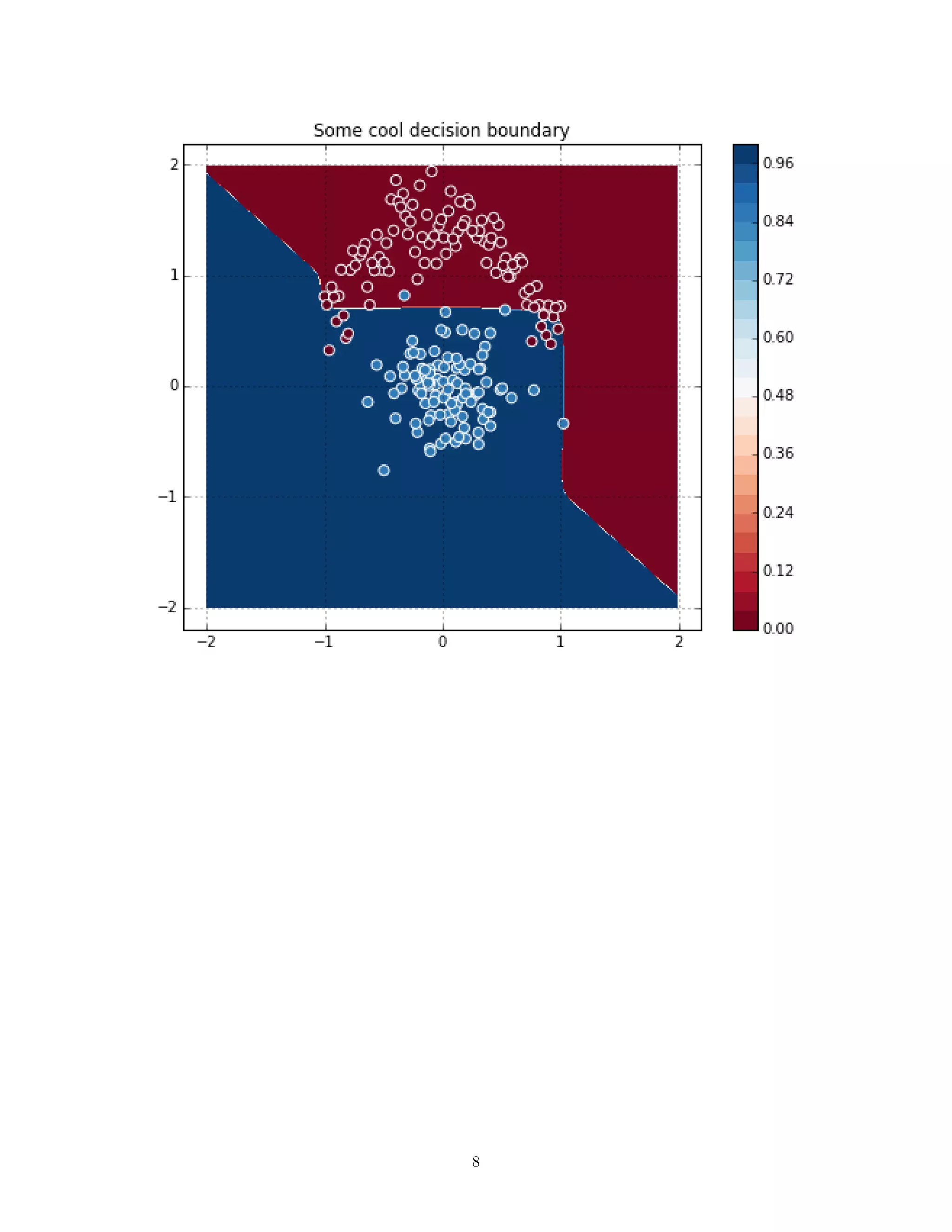
In [64]: predict = theano.function(
[X],
linear > 0
)
In [72]: preds = predict(grid_arr)
plot_decision(preds)
7

8. 8