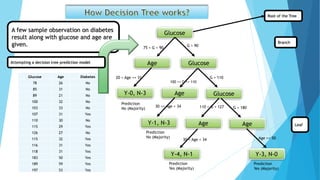
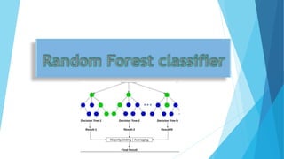
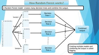
The document presents data on glucose levels, ages, and diabetes status for 15 individuals. It then shows how this data could be used to build a decision tree model to predict diabetes status based on glucose level and age ranges. The decision tree is split into branches and leaves based on thresholds for glucose and age. For example, one node examines individuals aged 30-34 and splits them based on glucose levels of 110-127 or greater than 180. The document also discusses concepts like information gain, entropy, and gini impurity that are used to determine the optimal splits in decision trees. It introduces the random forest technique of creating many decision trees and combining their predictions.

2. Glucose Age Diabetes
78 26 No
85 31 No
89 21 No
100 32 No
103 33 No
107 31 Yes
110 30 No
115 29 Yes
126 27 No
115 32 Yes
116 31 Yes
118 31 Yes
183 50 Yes
189 59 Yes
197 53 Yes
Glucose
Age Glucose
75 < G < 90
G > 90
20 < Age <= 31
Y-0, N-3
Prediction
No (Majority)
100 <= G <= 110
G > 110
Y-1, N-3
Prediction
No (Majority)
Age
30 <= Age < 34
Age
Glucose
110 < G < 127 G > 180
Age
Y-4, N-1
Prediction
Yes (Majority)
Age >= 50
Y-3, N-0
Prediction
Yes (Majority)
A few sample observation on diabetes
result along with glucose and age are
given.
Attempting a decision tree prediction model
30 < Age < 34
Root of the Tree
Branch
Leaf

3.  In the last slide example, the first split divided the into groups of 12 and 3.
 What if decision tree is creating a split for each sample?
 Then for the samples from train data, model can do accurate predictions.
 But for other data, model may perform worse.
 It is better to do the branch split with a minimum number of samples greater
than 1. (Default value is 2)
 We can control minimum sample split count of decision tree model with help
of “min_samples_split” argument.
Glucose
75 < G < 90
G > 90
No. of
samples = 3
No. of
samples = 12
 The samples count in last splits (leaf of decision tree) is also important for the
model
 Default value for minimum sample count in leaf of decision tree is 1.
 We can control the minimum count of samples in a decision tree model with
help of “min_samples_leaf” argument.

4.  Entropy is the measures of impurity, disorder or uncertainty in a bunch of
examples.
 In a decision tree it is the impurity in the split.
 Entropy value ranges from 0 to 1. Maximum impurity represents 1.
Entropy H(s) = -P(Yes) * log2(P(Yes)) -P(No) * log2(P(No))
Possible split with 6 samples (label “Yes” or “No”) with entropy in each split are shown below.
Entropy in case of more than 2 labels
Gini
Gini is another method of
impurity measure in the
decision tree split.
Gini = 1- (P(Yes)^2 + P(No)^2)
In case of more than 2 labels
Gini = 1 - ∑ (Pi)^2
No. of “Yes” No. of “No” P(Yes) P(No) Entropy Notes
0 6 0 1 0 pure split
1 5 0.17 0.83 0.65
2 4 0.33 0.67 0.92
3 3 0.5 0.5 1 maximum imprity
4 2 0.67 0.33 0.92
5 1 0.83 0.17 0.65
6 0 1 0 0 pure split
Gini
0
0.28
0.44
0.50
0.44
0.28
0

5. Information Gain helps to measure the reduction in entropy or surprise by splitting a dataset according to a given value of a random variable.
Information Gain IG(S, a) = H(S) – H(S | a)
IG(S, a) = information for the dataset S for the variable a
H(S) = the entropy for the dataset before any change
H(S | a) is the conditional entropy for the dataset given the variable a.
A larger information gain suggests a lower entropy group or groups of samples.
Overall Entropy = -(8/15)*log2(8/15) – (7/15) * log2(7/15) = 0.996
Feature - Gender:
Entropy of ‘Male’ = -(4/8)*log2(4/8)-(4/8)*log2(4/8) = 1
Entropy of ‘Female’ = -(4/7)*log2(4/7)-(3/7)*log2(3/7) = 0.985
Weighted entropy = (8/15)*1 + (7/15)*0.985 = 0.993
Information Gain for gender feature = 0.996 – 0.993 = 0.003
Information Gain for exercise feature = 0.996 – 0.884 = 0.112
Gender Exercise Diabetes
Male Regular No
Female Irregular No
Male Regular No
Male Regular No
Female No No
Male Irregular Yes
Female No No
Female Regular Yes
Male Regular No
Female Regular Yes
Female Regular Yes
Female Irregular Yes
Male Irregular Yes
Male No Yes
Male Irregular Yes

7. A Random Forest model creates many decision trees and combine the output.
x1 x2 x3 x4 x5 y
1
2
3
4
5
6
7
8
9
10
11
12
13
14
15
16
17
x1 x2 x3
1
2
3
4
x4 x5 y
13
14
15
16
17
x3 x4 x5 y
1
9
10
11
12
13
x1 x2 x3 y
1
2
3
4
Sample-1
Sample-2
Sample-3
Sample-n
Decision
Tree-1
Decision
Tree-2
Decision
Tree-3
Decision
Tree-n
Combined
output
M
A
J
O
R
I
T
Y
Creating multiple models and
combining the output is called
Bagging.

8. Number of trees in Random Forest can be managed by “n_estimators” argument.
Default number of trees is 100.
Random Forest reduces overfitting in decision trees and helps to improve the
accuracy.