Hypothesis testing for parametric data (1)

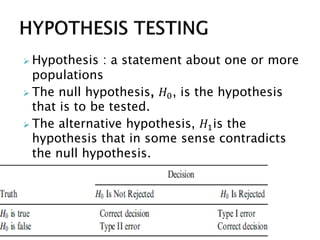
1.  Hypothesis : a statement about one or more
populations
 The null hypothesis, 𝐻0, is the hypothesis
that is to be tested.
 The alternative hypothesis, 𝐻1is the
hypothesis that in some sense contradicts
the null hypothesis.

2.  Variable :characteristic that we would like to
measure on individuals.
 Data :measurements recorded on individuals
 Dependent: outcome
 Independent : influence on the outcome

4. Steps in hypothesis testing
1.State the null &alternative hypothesis
2.Decide one or two sides test
3.Select the test statistic
4.Select the confidence level, establish
cut-off level and draw the acceptance
and rejection region
5.Compute the test statistic
6.Plot the test statistic in the curve and
make the conclusions

5. Using P-value to make a decision about whether to
reject, or not reject, your null hypothesis

6. Example: Interpreting a p-value – blood pressure
before and after exercise
In the example of examining change in blood pressure
before and after exercise in 16 men the p-value was
less than 0.001.
What does p < 0.001 mean?
Your results are unlikely when the null hypothesis is
true. Is this result statistically significant?
The result is statistically significant because the p-
value is less than the significance level α set at 5% or
0.05.
You decide?
That there is sufficient evidence to reject the null
hypothesis and accept the alternative hypothesis that
there is a difference (a rise) in the mean blood pressure
of middle-aged men before and after exercise.

7. Preparing for statistical testing
1) Identify type of data
2) Identify number of groups studied

9. One Group: Comparison of one sample mean with mean of
reference population
Z=
𝑿−𝝁
𝝈/ 𝒏
T=
𝑿−𝝁
𝑺/ 𝒏
X: sampe mean
s:estimated standard deviation
n: sample size
μ:hypothesized mean
Z or T test are basically the same
T test:
- If a sample is small (n< 30)
- If we do know the population standard deviation

10. Boys of a certain age have a mean weight of 8.5
Kg. An observation was made that in a city
neighborhood, children were underfed. As
evidence, all 25 boys in the neighborhood of
that age were weighed and found to have a
mean 𝑥 of 8.9 and a standard deviation s of 1.16
Kg . An application of the procedure above
yields
SE(𝑥)=
𝑆
𝑛
=
1.16
25
=0.232
t=
8.9−8.5
0.232
=1.724

11. The underfeeding complaint corresponds to the
one-sided alternative 𝐻𝐴: μ< 8.5so that we would
reject the null hypothesis if t ≤ tabulated value.
From Appendix C and with 24 degrees of freedom
(n-1) , we find that tabulated value= 1.71 under
the column corresponding to a 0.05 upper tail
area; the null hypothesis is rejected at the 0.05
level. In other words, there is enough evidence to
support the underfeeding complaint.

12. Comparing means two independent groups

13. This test is referred to as a two-sample t test
and its rejection region is determined using t
distribution at 𝑛1 + 𝑛2 − 2 degrees of freedom:
 For a one-tailed test, use the column
corresponding to an upper tail area of 0.05
and 𝐻0 is rejected if t≤ tatabulated value for
𝐻𝐴:μ1<μ2ort ≥tabulated value for 𝐻𝐴:μ1 > μ2
 For a two-tailed test or 𝐻𝐴 :μ1#μ2 , use the
column corresponding to an upper tail area of
0.025 and 𝐻0 is rejected if t ≤ tabulated value

14. In an attempt to assess the physical condition of joggers, a
sample of 𝑛1 =25 joggers was selected and their maximum
volume of oxygen uptake (V𝑂2) was measured with the
following results:
𝑥1=47.5 mL/kg 𝑠1= 4.8 mL/kg
Results for a sample of 𝑛2 =26 nonjoggers were
𝑥2= 37.5 mL/kg 𝑠2= 5.1 mL/kg
To proceed with the two-tailed, two-sample t test, we have

15. indicating a significant difference between
joggers and nonjoggers (at 49 degrees of
freedom , the tabulated t value, with an upper
tail area of 0.025, is about 2.0).

16. comparing means two dependent groups
It is applied to cases where each subject or
member of a group is observed twice (e.g., before
and after certain interventions),or matched pairs
are measured for the same continuous
characteristic.
What we really want to do is to compare the
means, before versus after or cases versus
controls, and use of the sample of differences
( 𝑑𝑖 , one for each subject, helps to achieve that.

17. The systolic blood pressures of n=12 women between the
ages of 20 and 35 were measured before and after
administration of a newly developed oral contraceptive:
SubjectBefore After Differences (𝑑𝑖) 𝑑𝑖
2
1 122 127 5 25
2 126 128 2 4
3 132 140 8 64
4 120 119 -1 1
5 142 145 3 9
6 130 130 0 0
7 142 148 6 36
8 137 135 -2 4
9 128 129 1 1
10 132 137 5 25
11 128 128 0 0
12 129 133 4 16
31 185

18. 𝑑=
31
12
=2.58 mm Hg
=
𝑑2 − 𝑑 2/𝑛
𝑛−1
=
185− 31 2/12
11
=9.54
𝒔𝒅=3.09
SE(𝑑)=
3.09
12
= 0.89 t=
2.58
0.89
=2.90
Degree of freedom=n-1 =12-1=11
Using the column corresponding to the upper tail area of
0.05 in Appendix C, we have a tabulated value of 1.796 for
11 df. Since t= 2.90 >1.796 we conclude that the null
hypothesis of no blood pressure change should be rejected
at the 0.05 level; there is enough evidence to support the
hypothesis of increased systolic blood pressure (one-sided
alternative).

20. Exercise : Vision, especially visual acuity, depends on a number of
factors. A study was undertaken in to determine the effect of
one of these factors: racial variation. Visual acuity of recognition
as assessed in clinical practice has a defined normal value of
20/20 (or zero on the log scale). The following summarize the
data on monocular visual acuity (expressed on a log scale).