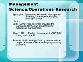
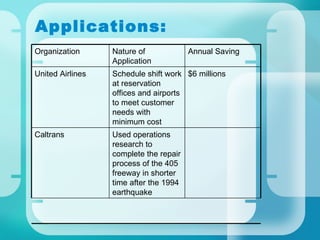
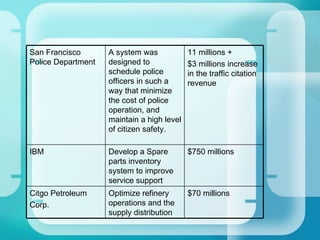
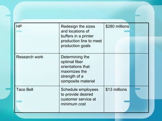
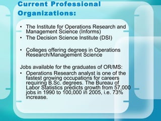
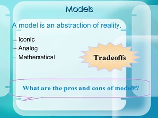
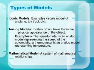
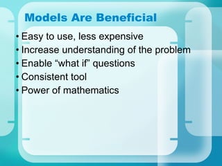
The document provides an overview of management science/operations research including: - A brief history noting early developments and contributors. - Applications across various industries showing cost savings and increased revenues. - Current professional organizations and typical jobs for graduates. - How management science techniques can help with system design, operation, and decision making. - The benefits and tradeoffs of different model types like iconic, analog, and mathematical models.

1. Management Science Introduction

2. Management Science/Operations Research Synonyms: Operations Research, Management Science, Quantitative Analysis, Decision Science History: Early 1900s:Frederic Taylor provided the foundation for the use of quantitative methods in management. About 1947: Modern development of OR/MS during world war II Summer 1947: George Dantzig developed the simplex method to solve linear programming problems.

3. First conference on linear programming First book of operations research Management Science: is a scientific approach for solving management problems.

4. Applications: Used operations research to complete the repair process of the 405 freeway in shorter time after the 1994 earthquake Caltrans $6 millions Schedule shift work at reservation offices and airports to meet customer needs with minimum cost United Airlines Annual Saving Nature of Application Organization

5. 11 millions + $3 millions increase in the traffic citation revenue A system was designed to schedule police officers in such a way that minimize the cost of police operation, and maintain a high level of citizen safety. San Francisco Police Department $70 millions Optimize refinery operations and the supply distribution Citgo Petroleum Corp. $750 millions Develop a Spare parts inventory system to improve service support IBM

6. $13 millions Schedule employees to provide desired customer service at minimum cost Taco Bell Determining the optimal fiber orientations that maximizes the strength of a composite material Research work $280 millions Redesign the sizes and locations of buffers in a printer production line to meet production goals HP

7. Current Professional Organizations: The Institute for Operations Research and Management Science (Informs) The Decision Science Institute (DSI) Colleges offering degrees in Operations Research/Management Science Jobs available for the graduates of OR/MS: Operations Research analyst is one of the fastest growing occupations for careers requiring B.Sc. degrees. The Bureau of Labor Statistics predicts growth from 57,000 jobs in 1990 to 100,000 in 2005, i.e. 73% increase.

8. What can management Science Techniques do? 1. System Design – capacity – location – arrangement of departments – product and service planning – acquisition and placement of equipment

9. Decision Making 2. System operation – personnel – Inventory – Scheduling – Project management Quality assurance –

10. Models A model is an abstraction of reality. What are the pros and cons of models? Tradeoffs – Iconic – Analog – Mathematical

11. Types of Models Iconic Models: Examples - scale model of airplane, toy truck etc. Analog Models : models do not have the same physical appearance of the object. Examples – The speedometer is an analog model representing the speed of the automobile, a thermometer is an analog model representing temperature. Mathematical Model : A system of mathematical relationships.

12. Models Are Beneficial Easy to use, less expensive Increase understanding of the problem Enable “what if” questions Consistent tool Power of mathematics

13. Quantitative Approaches Linear programming Integer programming Nonlinear programming Goal programming Queuing Techniques Project models Statistical models

14. Systems Approach “ The whole is greater than the sum of the parts .” Suboptimization

15. Pareto Phenomenon A few factors account for a high percentage of the occurrence of some event(s). 80/20 Rule - 80% of problems are caused by 20% of the activities. How do we identify the vital few?

16. Quantitative Analysis Approach Identify Problem Problem definition/Problem Statement Model development (Problem Formulation) Model Solution 5. Data Preparation

17. Quantitative Analysis Approach (continued) 6. Model Solution -Graphical Approach -Computer Approach 7. Report Generation 8. Result implementation

18. Mathematical Model Development: Step 1: Understand the problem. Step 2: Define the controllable inputs (decision variables) Step 3: Identify and model the Criterion (objective function) Step 4: Identify and model the restrictions (constraints) Step 5: Identify the upper/lower bounds.

19. Product Mix Example- Problem # 13- Pg. 41 The Electrotech Corporation manufactures twoindustrial-sized electrical devices: generators and alternators. Both of the products require wiring and testing during the assembly process. Each generator requires 2 hours of wiring and 1 hour of testing and can be sold for a $250 profit. Each alternator requires 3 hours of wiring and 2 hours of testing and can be sold for a $150 profit. There are 260 hours of wiring time and 140 hours of testing time available in the next production period and Electrotech would like to maximize profit. a) Formulate an LP model for this problem. b) Sketch the feasible region for this problem. c) Determine the optimal solution to this problem.

20. Example – 2.5 – Pg. 20 Blue Ridge Hot Tubs manufactures and sells two models of hot tubs: the Aqua-Spa and the Hydro-Lux. Howie Jones, the owner and manager of the company, needs to decide how many of each type of hot tub to produce during his next production cycle. Howie buys prefabricated fiberglass hot tub shells form a local supplier and adds the pump and tubing to the shells to create his hot tubs. (This supplier has the capacity to deliver as many hot tub shells as Howie needs.) Howie installs the same type of pump into both hot tubs. He will have only 200 pumps available during his next production cycle. From a manufacturing standpoint, the main difference between two models of hot tubs is the amount of tubing and labor required. Each Hydro-Lux requires 6 hours of labor and 16 feet of tubing available during the next production cycle. Howie earns a profit of $350 on each Aqua-Spa he sells and $350 on each Aqua-Spa he sells and $300 on each Hydro-Luxes should Howie produces if he wants to maximize his profits during the next production cycle?

21. Example 3-1/Practical MSCI The Monet Company produces four type of picture frames, which we label 1, 2, 3, 4. The four types of frames differ with respect to size, shape and materials used. Each type requires a certain amount of skilled labor, metal, and glass as shown in this table. The table lists the unit selling price Monet charges for each type of frame.

22. Example 3-1/Practical MSCI 21.50 2 2 2 Frame 4 29.25 1 1 3 Frame 3 12.50 2 2 1 Frame 2 28.50 6 4 2 Frame 1 Sale Price Glass Ounces Metal ounces Labor hr

23. Example 3-1/Practical MSCI During the coming week Monet can purchase up to 4000 hours of skilled labor, 6000 ounces of metal, and 10,000 ounces of glass. The unit costs are $8.00 per labor hour, $0.50 per ounce of metal, and $0.75 per ounce of glass. Also, market constraints are such that it is impossible to sell more than 1000 type 1 frames, 2000 type 2, frames, 500 type 3 frames, and 1000 type 4 frames. The company wants to maximize its weekly profit.

24. Example 3-1/Practical MSCI In the traditional algebraic solution method we first identify the decision variables. In this problem they are the number of frames of type 1, 2, 3, and 4 to produce. We label these x 1 , x 2 , x 3 , x 4 . Next we write total profit and the constraints in terms of the x ’s. Finally, since only nonnegative amounts can be produced, we add explicit constraints to ensure that the x ’s are nonnegative.

25. Example 3-1/Practical MSCI The resulting algebraic formulation is shown below: Maximize 6 x 1 + 2 x 2 + 4 x 3 + 3 x 4 (profit objective) Subject to 2 x 1 + x 2 + 3 x 3 + 2 x 4  4000 (labor constraint) 4 x 1 + 2 x 2 + x 3 + 2 x 4  10,000 (glass constraint) x 1  1000 (frame 1 sales constraints) x 2  2000 (frame 2 sales constraints) x 3  500 (frame 3 sales constraints) x 4  1000 (frame 4 sales constraints) x 1 , x 2 , x 3 , x 4  0 (nonnegativity constraint)

26. A Multiperiod Production Problem Example 3.3 Winston/Albright Page 91 The Pigskin Company produces footballs. Pigskin must decide how many footballs to produce each month. It has decided to use a 6-month planning horizon. The forecasted demands for the next 6 months are 10,000, 15,000, 30,000, 35,000, 25,000 and 10,000. Pigskin wants to meet these demands on time, knowing that it currently has 5000 footballs in inventory and that it can use a given month’s production to help meet the demand for that month.

27. Example 3.3 During each month there is enough production capacity to produce up to 30,000 footballs, and there is enough storage capacity to store up to 10,000 footballs at the end of the month, after demand has occurred. The forecasted production costs per football for the next 6 months are $12.50, $12.55, $12.70, $12.80, $12.85, and $12.95, respectively. The holding cost per football held in inventory at the end of the month is figured at 5% of the production cost for that month.

28. Example 3.3 In the traditional algebraic formulation, the decision variables are the production quantities for the 6 months, labeled P 1 through P 6 . It is convenient to let I 1 through I 6 be the corresponding end-of-month inventories (after the demand has occurred). For example, I 3 is the number of footballs left over at then end of month 3. Therefore, the obvious constraints are on production and inventory storage capacities: P j  300 and I j  100 for each month j , 1  j  6.

29. Example 3.3 In addition to these constraints, we need balance constraints that relate the P ’s and I ’s. In any month the inventory from the previous month plus the current production must equal the current demand plus leftover inventory. If D j is the forecasted demand for month j , then the balance equation for month j is I j - 1 + P j = D j + I j .

30. Example 3.3 The first of these constraints, for month j = 1, uses the known beginning inventory, 50, for the previous inventory (the I j -1 term) By putting all variables ( P ’s and I ’s) on the left and all known values on the right (a standard LP convention), these balance constraints become P 1 – I 1 = 100-50 I 1 + P 2 – I 2 = 150 I 2 + P 3 – I 3 = 300 I 3 + P 4 – I 4 = 350 I 4 + P 5 – I 5 = 250 I 5 + P 6 – I 6 = 100

31. Employee Scheduling Example 4.1 Winston/Albright A post office requires different numbers of full-time employees on different days of the week. The number of full-time employees required each day is given in this table. Employee Requirements for Post Office Monday 17 Tuesday 13 Wednesday 15 Thursday 19 Friday 14 Saturday 16 Sunday 11

32. Example 4.1 Winston/Albright Union rules state that each full-time employee must work 5 consecutive days and then receive 2 days off. For example, an employee who works Monday to Friday must be off Saturday and Sunday. The post office wants to meet its daily requirements using only full-time employees. Its objective is to minimize the number of full-time employees that must be hired.

33. To model the Post Office problem with a spreadsheet, we must keep track of the following: Number of employees starting work on each day of the week Number of employees working each day Total number of employees It is important to keep track of the number of employees starting work each day, because this is the only way to incorporate the fact that workers work 5 consecutive days.

34. Aggregate Planning Models Example 4.2 Winston/Albright During the next four months the SureStep Company must meet (on time) the following demands for pairs of shoes: 3,000 in month 1; 5,000 in month 2; 2,000 in month 3; and 1,000 in month 4. At the beginning of month 1, 500 pairs of shoes are on hand, and SureStep has 100 workers. A worker is paid $1,500 per month. Each worker can work up to 160 hours a month before he or she receives overtime. A worker is forced to work 20 hours of overtime per month and is paid $13 per hour for overtime labor.

35. Example 4.2 Winston/Albright It takes 4 hours of labor and $15 of raw material to produce a pair of shoes. At the beginning of each month workers can be hired or fired. Each hired worker costs $1600, and each fired worker cost $2000. At the end of each month, a holding cost of $3 per pair of shoes left in inventory is incurred.Production in a given month can be used to meet that month’s demand. SureStep wants to us LP to determine its optimal production schedule and labor policy.

36. Example 4.2 Winston/Albright To model SureStep’s problem with a spreadsheet, we must keep track of the following: Number of workers hired, fired, and available during each month. Number of pairs of shoes produced each month with regular time and overtime labor Number of overtime hours used each month Beginning and ending inventory of shoes each month Monthly costs and the total costs