INTRODUCTION
LEARNING OUTCOMES
CONTENT
❑ Definitionof Operation Research
❑ The Applications of Operation Research
❑ Problem Solving & Decision Making & Quantitative analysis
❑ Management Science Techniques
3.
DEFINITION
Operations Research (OR)is the methodology to allocate the available resources to the various
activities in a way that is most effective for the organization as a whole.
It is “applied to problems that concern how to conduct and coordinate the operations within an
organization.” By doing OR studies, we generate some suggestions for decision-makers.
Names of similar subjects/ideas:
Management science | Decision science | Optimization method/algorithm | Mathematical programming
INTRODUCTION
4.
From the early1900s: The use of quantitative methods in management (The scientific
management revolution - Frederic Winslow Taylor).
The World War II (01/09/1939–02/09/1945): deal with strategic and tactical problems faced by
the military.
The Post-World War II period: use of management science in nonmilitary application
+ Simplex method for solving linear programming problems - 1947 - George Dantzig
More recently: Data Science, Big Data, Machine Learning
INTRODUCTION
DEVELOPMENT HISTORY
5.
Today, everybody talksabout Business Analytics.
Master of Business Administration (MBA) becomes Master of Business Analytics
INTRODUCTION
BUSINESS ANALYTICS
6.
Two people aregoing to hold an event, and they need to complete some tasks.
One task must be assigned to exactly one person; one person can work on one task at a time.
How to assign the tasks so that they can complete all tasks the fastest?
What are the resources? What is the objective?
INTRODUCTION
EXAMPLE: JOB ALLOCATION
7.
n workers aregoing to complete m jobs in a project.
✔ Some jobs must be processed with precedence rules.
✔ Some jobs cannot be done by certain workers.
✔ Some jobs can be split and allocated to several workers.
✔ Some jobs require different processing time if allocated to different workers.
How many days does it take to complete this project?
INTRODUCTION
EXAMPLE: PROJECT MANAGEMENT
8.
How to setthe inventory level of product to maximize the total expected profit?
Suppose that there is ONLY ONE PRODUCT.
Prevent Understocking or Overstocking.
Data analysis: Estimate the random amount of demand during one order cycle time.
Operations research: According to the random amount of demand,
Find the inventory level to maximize the expected profit.
INTRODUCTION
EXAMPLE: PRODUCT INVENTORY
9.
How to setthe inventory levels of multiple products to maximize the total expected profit?
When we have MULTIPLE PRODUCTS.
Demand substitution: “There is no more Coke. How about Pepsi?”
Data analysis is difficult. Estimate the probability of demand substitution between A and B, which is the
probability for one to purchase B when A is sold out (or purchase A when B is sold out).
Operations research is also difficult. Given the substitution probabilities, find the best inventory levels of
all products.
INTRODUCTION
EXAMPLE: MULTI-PRODUCT INVENTORY
10.
You preparing forhiking. There are some useful items, but your backpack can only carry 5 kilograms.
An item cannot be split: Each item should be either chosen or discarded.
Which items should you bring to maximize the total value?
INTRODUCTION
EXAMPLE: KNAPSACK PROBLEM
11.
Key decisions:
✔ Howto deliver 6.5 millions items to more than 220 countries each day?
✔ In each region, where to build distribution hubs?
✔ In each distribution hub, how to classify and sort items?
✔ In each city, how to choose routes?
What do you need?
✔ Well-designed information systems.
✔ Operations Research!
INTRODUCTION
EXAMPLE: INDUSTRY APPLICATION
12.
Key decisions:
✔ Howto determine the cities to connect?
✔ How to schedule more than 2000 flights per day?
✔ How to assign crews to flights?
✔ How to reassign crews immediately when there is an emergency?
What do you need?
✔ Well-designed information systems.
✔ Operations Research!
INTRODUCTION
EXAMPLE: INDUSTRY APPLICATION
13.
Problem-solving: The processof identifying a difference between the actual and the desired state of
affairs and then taking action to resolve the difference.
Problem-solving process involves the following 7 steps:
1. Identify and define the problem.
2. Determine the set of alternative solutions.
3. Determine the criterion or criteria that will be used to evaluate the alternatives.
4. Evaluate the alternatives.
5. Choose an alternative (MAKE THE DECISION)
6. Implement the selected alternative.
7. Evaluate the results to determine whether a satisfactory solution has been obtained.
Decision making is the term generally associated with the first 5 steps of the problem-solving process.
INTRODUCTION
PROBLEM SOLVING AND DECISION MAKING
QUANTITATIVE ANALYSIS mightbe used when the problem is:
COMPLEX | IMPORTANT | NEW | REPETITIVE
INTRODUCTION
QUANTITATIVE ANALYSIS AND DECISION MAKING
16.
QUANTITATIVE ANALYSIS: Concentrateon the quantitative facts or data associated
with the problem and develop MATHEMATICAL EXPRESSIONS that describe the
objectives, constraints, and other relationships that exist in the problem.
Let x indicate the number of units produced each week: VARIABLE
The profit equation P = 10x: OBJECTIVE FUNCTION for a firm attempting to maximize profit.
A production capacity CONSTRAINT: 5 hours are required to produce each unit and only 40 hours
of production time are available per week.
INTRODUCTION
QUANTITATIVE ANALYSIS: MODEL DEVELOPMENT
LINEAR PROGRAMMING isa problem-solving approach developed for situations involving maximizing or minimizing a linear
function subject to linear constraints that limit the degree to which the objective can be pursued.
INTEGER LINEAR PROGRAMMING is an approach used for problems that can be set up as linear programs, with the additional
requirement that some or all of the decision variables be integer values.
DISTRIBUTION AND NETWORK MODELS A network is a graphical description of a problem consisting of circles called nodes
that are interconnected by lines called arcs (supply chain design, information system design, and project scheduling…).
NONLINEAR PROGRAMMING is a technique for maximizing or minimizing a nonlinear function subject to nonlinear
constraints.
PROJECT SCHEDULING: In many situations, managers are responsible for planning, scheduling, and controlling projects that
consist of numerous separate jobs or tasks performed by a variety of departments, individuals, and so forth. The PERT (Program
Evaluation and Review Technique) and CPM (Critical Path Method) techniques help managers carry out their project scheduling
responsibilities.
INVENTORY MODELS are used by managers faced with the dual problems of maintaining sufficient inventories to meet demand
for goods and, at the same time, incurring the lowest possible inventory holding costs.
WAITING-LINE | QUEUEING MODELS have been developed to help managers understand and make better decisions concerning
the operation of systems involving waiting lines.
SIMULATION is a technique used to model the operation of a system. This technique employs a computer program to model the
operation and perform simulation computations.
DECISION ANALYSIS can be used to determine optimal strategies in situations involving several decision alternatives and an
uncertain or risk-filled pattern of events.
GOAL PROGRAMMING is a technique for solving multicriteria decision problems, usually within the framework of linear
programming.
ANALYTIC HIERARCHY PROCESS This multicriteria decision-making technique permits the inclusion of subjective factors in
arriving at a recommended decision.
FORECASTING are techniques that can be used to predict future aspects of a business operation.
MARKOV PROCESS MODELS are useful in studying the evolution of certain systems over repeated trials. Markov processes have
been used to describe the probability that a machine, functioning in one period, will function or break down in another period.
INTRODUCTION
MANAGEMENT SCIENCE TECHNIQUES
20.
PART 2: LINEARPROGRAMMING
OPERATIONS RESEARCH
TRUNG-HIEP BUI
scv.udn.vn/buitrunghiep | hiepbt@due.udn.vn | 0935-743-555
21.
LINEAR
PROGRAMMING
CONTENT
LEARNING OUTCOMES
❑ Introductionto Linear Programming
❑ General Linear Programming Notations
❑ A Simple Maximization Problem
❑ Graphical Solution Procedure
❑ Extreme Points and the Optimal Solutions
❑ Computer application for solving Linear problems
22.
LINEAR
PROGRAMMING
1. A manufacturerwants to develop a production schedule and an inventory policy that will satisfy sales
demand in future periods. Ideally, the schedule and policy will enable the company to satisfy demand and at the
same time minimize the total production and inventory costs.
2. A financial analyst must select an investment portfolio from a variety of stock and bond investment
alternatives. The analyst would like to establish a portfolio that maximizes the return on investment.
3. A marketing manager wants to determine how best to allocate a fixed advertising budget among
alternative advertising media such as radio, television, online, and magazines. The manager would like to
determine the media mix that maximizes advertising effectiveness.
4. A company has warehouses in a number of locations. For a set of customer demands, the company would
like to determine how much each warehouse should ship to each customer so that total transportation costs are
minimized.
SOME LINEAR PROGRAMMING PROBLEMS
23.
LINEAR
PROGRAMMING
A manufacturer ofgolf equipment produces 02 types of golf bag (Standard | Deluxe).
A profit contribution of $10 for every standard bag and $9 for every deluxe bag produced.
A SIMPLE MAXIMIZATION PROBLEM
CONSTRAINTS
Nonnegativity constraints: nonnegative values for the decision variables.
24.
LINEAR
PROGRAMMING
A manufacturer ofgolf equipment produces 02 types of golf bag (Standard | Deluxe).
A profit contribution of $10 for every standard bag and $9 for every deluxe bag produced.
A SIMPLE MAXIMIZATION PROBLEM: PROBLEM FORMULATION
Define the Decision Variables
LINEAR
PROGRAMMING
The Cutting andDyeing Constraint Line
A SIMPLE MAXIMIZATION PROBLEM: GRAPHICAL SOLUTION PROCEDURE
Infeasible solution
Feasible solution
Feasible region
Infeasible region
LINEAR
PROGRAMMING
1800$ | 3600$| 5400$ Profit Lines
A SIMPLE MAXIMIZATION PROBLEM: GRAPHICAL SOLUTION PROCEDURE
Let P represent Total Profit Contribution
The slope-intercept form
of the linear equation relating S and D.
32.
LINEAR
PROGRAMMING
Optimal Solution
A SIMPLEMAXIMIZATION PROBLEM: GRAPHICAL SOLUTION PROCEDURE
Optimal solution point is on both:
The Cutting and Dying constraint line
The Finishing constraint line
The slope-intercept form
of the linear equation relating S and D.
33.
LINEAR
PROGRAMMING
SLACK VARIABLE
Optimal Solution:S = 540 and D =252
The 120 hours of unused sewing time and 18 hours of unused inspection and packaging time
are referred to as slack for the two departments.
34.
LINEAR
PROGRAMMING
SLACK VARIABLE
Whenever alinear program is written in a form with all constraints expressed as equalities,
it is said to be written in STANDARD FORM.
SLACK VARIABLES are added to the formulation of a linear
programming problem to represent the slack, or idle capacity.
Unused ((idle) capacity makes no contribution to profit;
thus, slack variables have coefficients of zero in the objective function.
Adding 4 slack variables, denoted as S1, S2, S3, and S4.
Binding constraint
Non-binding constraint
35.
LINEAR
PROGRAMMING
EXTREME POINTS ANDTHE OPTIMAL SOLUTION
Suppose that the profit contribution for standard golf bag is reduced from $10 to $5 per bag,
while the profit contribution for the deluxe golf bag and all the constraints remain unchanged.
The revised objective function: Max (5S + 9D)
Without any change in the constraints, the feasible region does not change.
However, the profit lines have been altered to reflect the new objective function.
The reduced profit contribution
for the standard bag caused a
change in the optimal solution.
36.
LINEAR
PROGRAMMING
EXTREME POINTS ANDTHE OPTIMAL SOLUTION
The optimal solution to a linear program can be found at an extreme point of the feasible region.
We can find the optimal solution by evaluating the 5 extreme-point solutions
and selecting the one that provides the largest profit contribution.
LINEAR
PROGRAMMING
A manufacturer needs02 types of products (A | B).
A SIMPLE MINIMIZATION PROBLEM
VARIABLES
Demand Processing time
per gallon
Production cost
per gallons
Product A ≥ 125 gallons 2 hours 2 $
Product B 1 hours 3 $
Total ≥ 350 gallons ≤ 600 hours
MATHEMATICAL MODEL
LINEAR
PROGRAMMING
SURPLUS VARIABLE
Optimal Solution:A = 250 and B = 100
The production of product A exceeds its minimum level by 250 - 125 = 125 gallons.
This excess production for product A is referred to as SURPLUS.
In linear programming terminology, any excess quantity corresponding to
a ≥ constraint is referred to as SURPLUS.
45.
LINEAR
PROGRAMMING
SLACK VARIABLE &SURPLUS VARIABLE
With a ≤ constraint,
a SLACK variable can be added to the left-hand side of the inequality
to convert the constraint to equality form.
With a ≥ constraint,
a SURPLUS variable can be subtracted from the left-hand side of the inequality
to convert the constraint to equality form.
46.
LINEAR
PROGRAMMING
SLACK VARIABLE &SURPLUS VARIABLE
✔ SURPLUS variables are given a coefficient of zero in the objective function because they have no effect on its value.
✔ Adding 02 SURPLUS variables, denoted as S1, S2 (≥ constraint) and 01 SLACK variable, denoted as S3 (≤ constraint)
✔ Whenever a linear program is written in a form with all constraints expressed as equalities, it has STANDARD FORM.
Remind: Optimal solution:S = 540 standard bags and D = 252 deluxe bags,
was based on profit contribution figures of $10 per standard bag and $9 per deluxe bag
SENSITIVITY ANALYSIS
Sensitivity analysis is the study of how the changes in the coefficients of an optimization model
affect the optimal solution. Using sensitivity analysis, we can answer questions such as the following:
1. How will a change in the coefficient of the objective function affect the optimal solution?
2. How will a change in the right-hand-side value for a constraint affect the optimal solution?
DEFINITION & PROPERTIES
54.
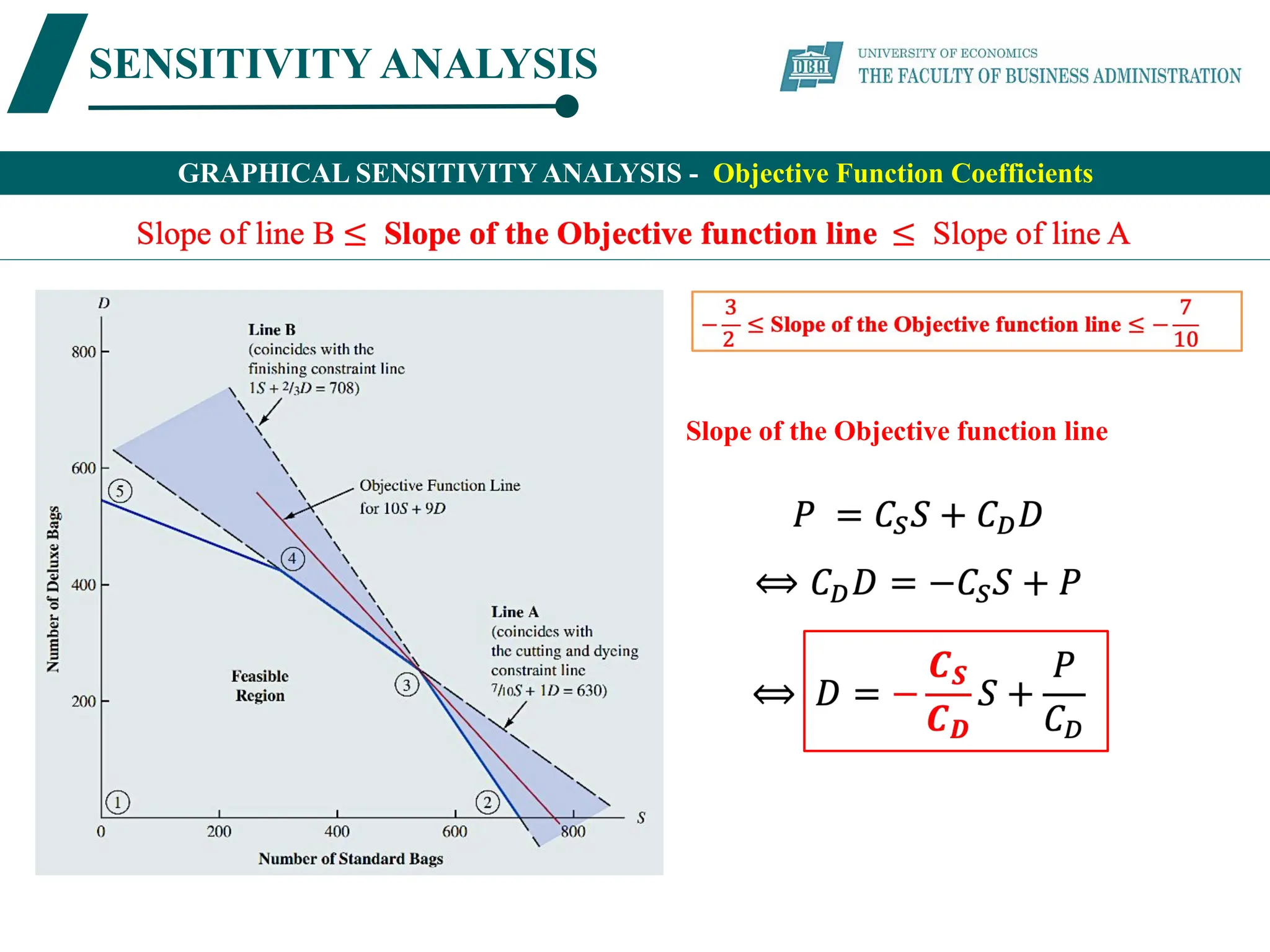
SENSITIVITY ANALYSIS
The rangeof optimality for each objective function coefficient provides the range
of values over which the current solution will remain optimal.
Extreme point (3) will be the optimal solution as long as:
GRAPHICAL SENSITIVITY ANALYSIS - Objective Function Coefficients
SENSITIVITY ANALYSIS
Sensitivity analysisis the study of how the changes in the coefficients of an optimization model
affect the optimal solution. Using sensitivity analysis, we can answer questions such as the following:
1. How will a change in the coefficient of the objective function affect the optimal solution?
2. How will a change in the right-hand-side value for a constraint affect the optimal solution?
SENSITIVITY ANALYSIS - Right-Hand Side
Optimal solution: S = 540 standard bags and D = 252 deluxe bags,
was based on profit contribution figures of $10 per standard bag and $9 per deluxe bag
63.
SENSITIVITY ANALYSIS
The RHSof the “Cutting and Dyeing constraint” is changed from 630 to 640
GRAPHICAL SENSITIVITY ANALYSIS - Right-Hand Side
64.
SENSITIVITY ANALYSIS
The RHSof the “Cutting and Dyeing constraint” is changed from 630 to 640
GRAPHICAL SENSITIVITY ANALYSIS - Right-Hand Side – Dual value
SENSITIVITY ANALYSIS
The reducedcost of a variable is equal to the dual value for the nonnegativity constraint
associated with that variable.
SENSITIVITY ANALYSIS - Right-Hand Side – Reduced Cost
67.
SENSITIVITY ANALYSIS
S (currentprofit coefficient of 10), has an Allowable increase of 3.5 and an Allowable decrease of 3.7.
If the profit contribution of the Standard bag is between 10 - 3.7 = $ 6.3 and 10 + 3.5 = $ 13.5,
the production of (S= 540; D= 252) will remain the optimal solution.
SENSITIVITY ANALYSIS -
Ranges for Objective Function Coefficients and the RHS of the constraints
68.
SENSITIVITY ANALYSIS
If theconstraint RHS is not increased (decreased) by more than the Allowable increase (decrease),
the associated dual value gives the exact change in the value of the Optimal solution per unit increase
in the RHS.
SENSITIVITY ANALYSIS -
Ranges for Objective Function Coefficients and the RHS of the constraints
69.
SENSITIVITY ANALYSIS
Constraint 1:Dual value 4.375 is valid for RHS values within the range [495.6 ; 682.36364]
(630 – 134.4 = 495.6 ; 630 + 52.36364 = 682.36364)
SENSITIVITY ANALYSIS -
Ranges for Objective Function Coefficients and the RHS of the constraints
PART 4: DISTRIBUTIONAND NETWORK MODELS
OPERATIONS
RESEARCH
TRUNG-HIEP BUI
scv.udn.vn/buitrunghiep | hiepbt@due.udn.vn | 0935-743-555
75.
CONTENT
❑ Supply ChainModels
❑ Assignment Problem
❑ Shortest-Route Problem
❑ Maximal Flow Problem
❑ A Production and Inventory Application
DISTRIBUTION AND NETWORK MODELS
LEARNING OUTCOMES
76.
TRANSPORTATION PROBLEM
✔ Arisesfrequently in planning for the distribution
of goods/services from several supply locations
to several demand locations.
✔ The quantity of goods available at each supply
locations (origin) is limited.
✔ The quantity of goods needed at each of demand
locations (destinations) is known.
✔ The usual objective is to minimize the cost of
shipping goods from the origins to the
destinations.
DISTRIBUTION AND NETWORK MODELS
SUPPLY DEMAND
ORIGIN DESTINATION
SUPPLY CHAIN MODELS
77.
TRANSSHIPMENT PROBLEM
✔ Isan extension of the transportation problem.
✔ Add intermediate nodes (transhipment nodes).
✔ Shipments may be made between any pair of the
three general types of nodes.
✔ The supply available at each origin is limited.
✔ The demand at each destination is specified.
✔ The objective is to determine how many units
should be shipped over each arc in the network
so that all destination demands are satisfied with
the minimum possible transportation cost.
DISTRIBUTION AND NETWORK MODELS
SUPPLY DEMAND
ORIGIN TRANSSHIPMENT DESTINATION
SUPPLY CHAIN MODELS
78.
ASSIGNMENT PROBLEM
✔ Isan extension of the transportation problem.
✔ One agent is assigned to one and only one task.
✔ The objective is to set of assignments that will
optimize a stated objective, such as minimize
cost, minimize time, or maximize profits.
DISTRIBUTION AND NETWORK MODELS
SUPPLY CHAIN MODELS
79.
SUPPLY CHAIN MODELS
SHORTEST-ROUTEPROBLEM
✔ The objective is to determine the shortest route,
or path, between two nodes in a network
DISTRIBUTION AND NETWORK MODELS
MAXIMAL FLOW PROBLEM
✔ The objective is to determine the maximum
amount of flow (vehicles, messages, fluid, etc.)
that can enter and exit a network system in a
given period of time.
✔ Attempt to transmit flow through all arcs of the
network as efficiently as possible.
✔ The amount of flow is limited due to capacity
restrictions (flow capacity) on the various arcs
of the network.
80.
Proctor & Gamblemakes and markets over 300 brands of consumer goods worldwide.
The company had hundreds of suppliers, over 60 plants, 15 distributing centers, and over 1000
consumer zones. Managing item flows over the huge supply network is challenging!
✔ An LP/IP model helps.
✔ The special structure of network transportation must also be utilized.
200 million dollars are saved after an OR study! (https://doi.org/10.1287/inte.27.1.128)
DISTRIBUTION AND NETWORK MODELS
SUPPLY CHAIN MODELS
81.
A lot ofoperations are to transport items on a network.
Moving materials from suppliers to factories.
Moving goods from factories to distributing centers.
Moving goods from distributing centers to retail stores.
Sending passengers through railroads or by flights.
Sending data packets on the Internet.
Sending water through pipelines.
And many more.
A unified model, the minimum cost network flow (MCNF) model, covers many network operations.
It has some very nice theoretical properties.
It can also be used for making decisions regarding inventory, project management, job assignment,
facility location, etc.
DISTRIBUTION AND NETWORK MODELS
SUPPLY CHAIN MODELS
TRANSPORTATION PROBLEM
✔ Arisesfrequently in planning for the distribution
of goods/services from several supply locations
to several demand locations.
✔ The quantity of goods available at each supply
locations (origin) is limited.
✔ The quantity of goods needed at each of demand
locations (destinations) is known.
✔ The usual objective is to minimize the cost of
shipping goods from the origins to the
destinations.
DISTRIBUTION AND NETWORK MODELS
SUPPLY DEMAND
ORIGIN DESTINATION
SUPPLY CHAIN MODELS - TRANSPORTATION PROBLEM
84.
DISTRIBUTION AND NETWORKMODELS
SUPPLY CHAIN MODEL – TRANSPORTATION MODEL
Transportation Cost per Unit
85.
DISTRIBUTION AND NETWORKMODELS
SUPPLY CHAIN MODEL – TRANSPORTATION MODEL
The decision variables for a transportation problem having m origins
and n destinations are written as:
xij
: number of units shipped from origin i to destination j
(where i=1, 2, . . . , m and j= 1, 2, . . . , n)
DISTRIBUTION AND NETWORKMODELS
SUPPLY CHAIN MODEL – VARIATION OF BASIC TRANSPORTATION MODEL
• TOTAL SUPPLY not equal to TOTAL DEMAND
TOTAL SUPPLY > TOTAL DEMAND
• No modification in the LP formulation is
necessary.
• Excess supply will appear as SLACK in the
linear programming solution.
• SLACK for any particular origin can be
interpreted as the unused supply or amount not
shipped from the origin.
TOTAL SUPPLY < TOTAL DEMAND
• Add a dummy origin with a supply equal to the
difference between the total demand and the total
supply.
• Add an arc from the dummy origin to each destination.
• Assign a zero cost per unit to each arc leaving the
dummy origin (no shipments actually will be made
from the dummy origin).
• When the optimal solution is implemented, the
destinations showing shipments being received from the
dummy origin will be the shortfall or unsatisfied
demand of the destinations.
88.
DISTRIBUTION AND NETWORKMODELS
SUPPLY CHAIN MODEL – GENERAL LINEAR PROGRAMMING MODEL
• Route capacities or Route minimums or Unacceptable routes
89.
TRANSSHIPMENT PROBLEM
✔ Isan extension of the transportation problem.
✔ Add intermediate nodes (transhipment nodes).
✔ Shipments may be made between any pair of the
three general types of nodes.
✔ The supply available at each origin is limited.
✔ The demand at each destination is specified.
✔ The objective is to determine how many units
should be shipped over each arc in the network
so that all destination demands are satisfied with
the minimum possible transportation cost.
DISTRIBUTION AND NETWORK MODELS
SUPPLY DEMAND
ORIGIN TRANSSHIPMENT DESTINATION
SUPPLY CHAIN MODELS - TRANSSHIPMENT PROBLEM
90.
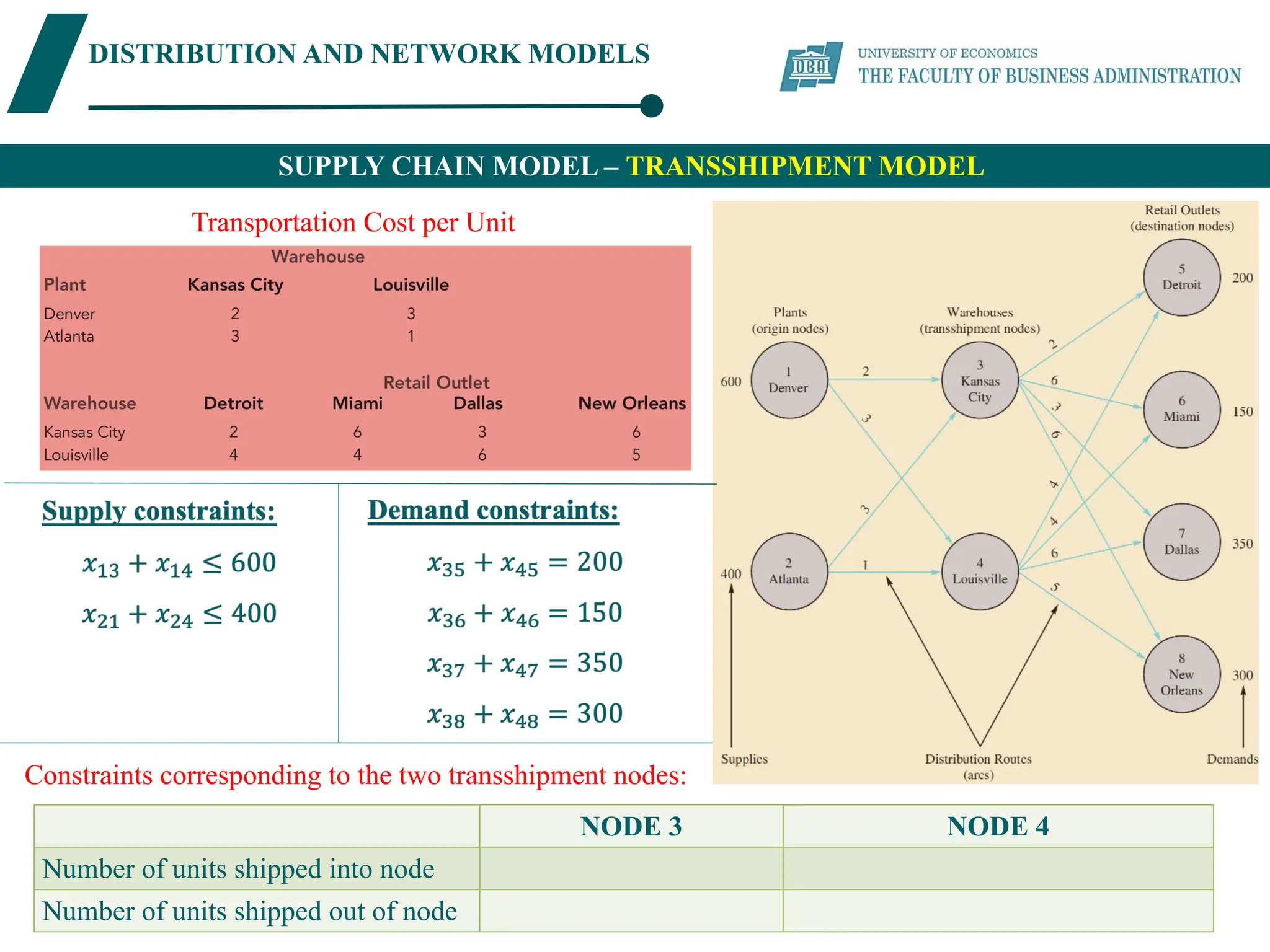
DISTRIBUTION AND NETWORKMODELS
SUPPLY CHAIN MODEL – TRANSSHIPMENT MODEL
Transportation Cost per Unit
Constraints corresponding to the two transshipment nodes:
NODE 3 NODE 4
Number of units shipped into node
Number of units shipped out of node
91.
DISTRIBUTION AND NETWORKMODELS
SUPPLY CHAIN MODEL – TRANSSHIPMENT MODEL
The objective function reflects the total shipping cost over the 12 shipping routes.
Combining the Objective function and Constraints leads to a 12-variable, 8-constraint LP model
of the transshipment problem.
92.
DISTRIBUTION AND NETWORKMODELS
SUPPLY CHAIN MODEL – TRANSSHIPMENT MODEL
550
50
400
200
150
350
300
93.
DISTRIBUTION AND NETWORKMODELS
SUPPLY CHAIN MODEL – VARIATION OF BASIC TRANSSHIPMENT MODEL
Suppose that it is possible to ship directly:
- from Atlanta to New Orleans at $4 / unit
- from Dallas to New Orleans at $1/ unit
ASSIGNMENT PROBLEM
✔ Isan extension of the transportation problem.
✔ One agent is assigned to one and only one task.
✔ The objective is to set of assignments that will
optimize a stated objective, such as minimize
cost, minimize time, or maximize profits.
DISTRIBUTION AND NETWORK MODELS
SUPPLY CHAIN MODELS - ASSIGNMENT PROBLEM
DISTRIBUTION AND NETWORKMODELS
SUPPLY CHAIN MODEL – ASSIGNMENT MODEL
SOLUTION
If ai
denotes the upper limit for the number of tasks
to which agent i can be assigned
A GENERAL LINEAR PROGRAMMING MODEL
99.
DISTRIBUTION AND NETWORKMODELS
SUPPLY CHAIN MODEL – SHORTEST-ROUTE PROBLEM
The shortest-route problem can be viewed as a transshipment problem
with one origin node (node 1), one destination node (node 6),
and four transshipment nodes (nodes 2, 3, 4, and 5).
100.
DISTRIBUTION AND NETWORKMODELS
SUPPLY CHAIN MODEL – SHORTEST-ROUTE PROBLEM
Origin node (node 1): Has a supply of 1 unit; Connected arc always go out.
Destination node (node 6): Has a demand of 1 unit; Connected arc always go into.
Four transshipment nodes (nodes 2, 3, 4, and 5): Two directed arcs connect between the pairs of transshipment nodes.
DISTRIBUTION AND NETWORKMODELS
SUPPLY CHAIN MODEL – SHORTEST-ROUTE PROBLEM - Constraints
The constraint for Node 1: x12
+ x13
= 1
The constraint for Node 6: x26
+ x46
+ x56
= 1
SUPPLY CHAIN MODELS- MAXIMAL FLOW PROBLEM
DISTRIBUTION AND NETWORK MODELS
MAXIMAL FLOW PROBLEM
✔ The objective is to determine the maximum
amount of flow (vehicles, messages, fluid, etc.)
that can enter and exit a network system in a
given period of time.
✔ Attempt to transmit flow through all arcs of the
network as efficiently as possible.
✔ The amount of flow is limited due to capacity
restrictions (flow capacity) on the various arcs
of the network.
107.
DISTRIBUTION AND NETWORKMODELS
SUPPLY CHAIN MODEL – MAXIMAL FLOW PROBLEM
Each arc’s flow direction is indicated, and the arc capacity (1.000 vehicles/hour) is shown next to each arc.
NORTH-SOUTH VEHICLE FLOW: 15.000 vehicles/hour
The maximum flow problem can be viewed as a capacitated transshipment model.
108.
DISTRIBUTION AND NETWORKMODELS
SUPPLY CHAIN MODEL – MAXIMAL FLOW PROBLEM
NORTH-SOUTH VEHICLE FLOW: 15.000 vehicles/hour
109.
DISTRIBUTION AND NETWORKMODELS
SUPPLY CHAIN MODEL – MAXIMAL FLOW PROBLEM
xij
: Amount of traffic from Node i to Node j.
NORTH-SOUTH VEHICLE FLOW: 15.000 vehicles/hour
The flow OUT for Node 1: x12
+ x13
+ x14
The flow IN for Node 1: x71
=> The constraint: x12
+ x13
+ x14
- x71
= 0
The objective function that maximizes the flow over the highway system is: Max x71
“Capacity on the arc” constraints:
110.
DISTRIBUTION AND NETWORKMODELS
SUPPLY CHAIN MODEL – MAXIMAL FLOW PROBLEM
NORTH-SOUTH VEHICLE FLOW: 15.000 vehicles/hour
111.
SUPPLY CHAIN MODELS– A PRODUCTION AND INVENTORY APPLICATION
DISTRIBUTION AND NETWORK MODELS
Determine how many products (yards of carpeting) to manufacture each quarter
to minimize the total production and inventory cost for the four-quarter period?
112.
SUPPLY CHAIN MODELS– A PRODUCTION AND INVENTORY APPLICATION
DISTRIBUTION AND NETWORK MODELS
We begin by developing a network representation of the problem.
Create 04 nodes corresponding to the production in each quarter.
For each production node: an outgoing arc to the demand node for the same period.
The flow on the arc represents the number of square yards of carpet manufactured for the period.
Create four nodes corresponding to the demand in each quarter
For each demand node: an outgoing arc represents the amount of inventory (square yards of carpet)
carried over to the demand node for the next period.
113.
SUPPLY CHAIN MODELS– A PRODUCTION AND INVENTORY APPLICATION
DISTRIBUTION AND NETWORK MODELS
The objective is to determine a production
scheduling and inventory policy that minimizes the
total production and inventory cost for the 4 quarters.
Min
2x15
+ 5x26
+ 3x37
+ 3x48
+ 0.25x56
+ 0.25x67
+ 0.25x78
114.
SUPPLY CHAIN MODELS– A PRODUCTION AND INVENTORY APPLICATION
DISTRIBUTION AND NETWORK MODELS
115.
PART 5: INTEGERLINEAR PROGRAMMING
OPERATIONS
RESEARCH
TRUNG-HIEP BUI
scv.udn.vn/buitrunghiep | hiepbt@due.udn.vn | 0935-743-555
116.
CONTENT
❑ Types ofInteger Linear Programming Models
❑ Graphical and Computer Solutions for an All-integer LP
❑ Application involving 0-1 Variables
❑ Modeling Flexibility Provided by 0-1 Integer Variables
DISTRIBUTION AND NETWORK MODELS
LEARNING OUTCOMES
117.
TYPES OF INTEGERLINEAR PROGRAMMING MODELS
DISTRIBUTION AND NETWORK MODELS
All-integer linear program LP RELAXATION Mixed-integer linear program
0-1 linear integer program
118.
GRAPHICAL AND COMPUTERSOLUTIONS FOR AN ALL-INTEGER LP
DISTRIBUTION AND NETWORK MODELS
BT has $2 million to purchase rental property (townhouse and apartment buildings).
- Each townhouse can be purchased for $282,000 and 05 townhouses are available.
- Each apartment building can be purchased for $400,000 and the is no limit quantity of apartments.
BT can devote up to 140 hours per month to managing these new properties.
- Each townhouse requires 4 hours per month.
- Each apartment building requires 40 hours per month.
The annual cash flow is estimated at $10,000 per townhouse and $15,000 per apartment.
BT would like to determine the number of townhouses (T) and the number of apartment buildings
(A) to purchase to maximise annual cash flow.
GRAPHICAL AND COMPUTERSOLUTIONS FOR AN ALL-INTEGER LP
DISTRIBUTION AND NETWORK MODELS
T = 2.479 ; A = 3.252
10(2.479) + 15(3.252) = 73.574 (k$)
Round the solution:
T = 2.479 ≈ 2; A = 3.252 ≈ 3
10(2) + 15(3) = 65 (k$)
(T = 3; A = 3): Infeasible solution
282(3) + 400(3) = 2046 (k$) > 2.000 (k$)
122.
GRAPHICAL AND COMPUTERSOLUTIONS FOR AN ALL-INTEGER LP
DISTRIBUTION AND NETWORK MODELS
T = 2.479 ≈ 2; A = 3.252 ≈3
10(2.479) + 15(3.252) = 73.574 (k$)
Round the solution:
T = 2.479 ≈ 2; A = 3.252 ≈3
10(2) + 15(3) = 65 (k$)
Optimal Integer solution:
(T = 4; A = 2):
10(4) + 15(2) = 70 (k$)
123.
GRAPHICAL AND COMPUTERSOLUTIONS FOR AN ALL-INTEGER LP
DISTRIBUTION AND NETWORK MODELS
T = 2.479 ≈ 2; A = 3.252 ≈3
10(2.479) + 15(3.252) = 73.574 (k$)
Round the solution:
T = 2.479 ≈ 2; A = 3.252 ≈3
10(2) + 15(3) = 65 (k$)
Optimal Integer solution:
(T = 4; A = 2):
10(4) + 15(2) = 70 (k$)
124.
APPLICATIONS INVOLVING 0-1VARIABLES – CAPITAL BUDGETING
DISTRIBUTION AND NETWORK MODELS
Faced with limited capital for the next 04 years, company needs to select the most profitable projects.
Present value*: The estimated net present value is the net cash flow discounted back to the beginning of year 1
The four 0-1 decision variables are:
P = 1 if the Plant expansion project is accepted; 0 if rejected
W = 1 if the Warehouse expansion project is accepted; 0 if rejected
M = 1 if the New machinery project is accepted; 0 if rejected
R = 1 if the New product research project is accepted; 0 if rejected
APPLICATIONS INVOLVING 0-1VARIABLES – FIXED COST PROBLEM
DISTRIBUTION AND NETWORK MODELS
03 materials are used to produce 03 products: Fuel additive, Solvent base, and Carpet cleaning fluid.
The following decision variables are used:
F = tons of fuel additive produced
S = tons of solvent base produced
C = tons of carpet cleaning fluid produced
PRODUCT
Profit
per ton of product
Quantity of material to produce a ton of product
Material 1 Material 2 Material 3
Fuel additive 40 0.4 0.6
Solvent base 30 0.5 0.2 0.3
Carpet cleaning fluid 50 0.6 0.1 0.3
Maximum available material
128.
APPLICATIONS INVOLVING 0-1VARIABLES – FIXED COST PROBLEM
DISTRIBUTION AND NETWORK MODELS
03 materials are used to produce 03 products: Fuel additive, Solvent base, and Carpet cleaning fluid.
PRODUCT
Profit
per ton of product
Quantity of material to produce a ton of product
Material 1 Material 2 Material 3
Fuel additive 40 0.4 0.6
Solvent base 30 0.5 0.2 0.3
Carpet cleaning fluid 50 0.6 0.1 0.3
Maximum available material
This LP formulation does not include a fixed cost for production setup of the products.
129.
APPLICATIONS INVOLVING 0-1VARIABLES – FIXED COST PROBLEM
DISTRIBUTION AND NETWORK MODELS
03 materials are used to produce 03 products: Fuel additive, Solvent base, and Carpet cleaning fluid.
PRODUCT
Profit
per ton of
product
Quantity of material
to produce a ton of product Setup
cost
Maximum
production
(tons)
Material 1 Material 2 Material 3
Fuel additive 40 0.4 0.6 200 50
Solvent base 30 0.5 0.2 0.3 50 25
Carpet cleaning fluid 50 0.6 0.1 0.3 400 40
Maximum available
material
The 0-1 variables can be used to incorporate the fixed setup costs into the production model.
SF = 1 if the fuel additive is produced; 0 if not
SS = 1 if the solvent base is produced; 0 if not
SC = 1 if the carpet cleaning fluid is produced; 0 if not
Using these setup variables, the total setup cost is: 200.SF + 50.SS + 400.SC
The objective function to include the setup cost: Max (40.F + 30.S + 50.C – 200.SF - 50.SS – 400.SC)
130.
APPLICATIONS INVOLVING 0-1VARIABLES – FIXED COST PROBLEM
DISTRIBUTION AND NETWORK MODELS
03 materials are used to produce 03 products: Fuel additive, Solvent base, and Carpet cleaning fluid.
PRODUCT
Profit
per ton of
product
Quantity of material
to produce a ton of product Setup
cost
Maximum
production
(tons)
Material 1 Material 2 Material 3
Fuel additive 40 0.4 0.6 200 50
Solvent base 30 0.5 0.2 0.3 50 25
Carpet cleaning fluid 50 0.6 0.1 0.3 400 40
Maximum available material
Using these setup variables, the total setup cost is: 200.SF + 50.SS + 400.SC
The objective function to include the setup cost: Max (40.F + 30.S + 50.C – 200.SF - 50.SS – 400.SC)
The constraints:
F ≤ 50.SF S ≤ 25.SS C ≤ 40.SC
SF, SS, SC = 0 or 1
131.
APPLICATIONS INVOLVING 0-1VARIABLES – FIXED COST PROBLEM
DISTRIBUTION AND NETWORK MODELS
PRODUCT
Profit
per ton of
product
Quantity of material
to produce a ton of product Setup
cost
Maximum
production
(tons)
Material 1 Material 2 Material 3
Fuel additive 40 0.4 0.6 200 50
Solvent base 30 0.5 0.2 0.3 50 25
Carpet cleaning fluid 50 0.6 0.1 0.3 400 40
Maximum available material
APPLICATIONS INVOLVING 0-1VARIABLES – DISTRIBUTION SYSTEM DESIGN
DISTRIBUTION AND NETWORK MODELS
Proposed plant
Annual fixed cost
($)
Annual capacity
(unit)
Shipping cost per unit ($)
from Plant to Distribution center
Boston Atlanta Houston
Detroit 175.000 10.000 5 2 3
Toledo 300.000 20.000 4 3 4
Denver 375.000 30.000 9 7 5
Kansas city 500.000 40.000 10 4 2
Current plant
ST. Louis 30.000 8 4 3
30.000 20.000 20.000
Annual
Demand
134.
APPLICATIONS INVOLVING 0-1VARIABLES – DISTRIBUTION SYSTEM DESIGN
DISTRIBUTION AND NETWORK MODELS
0-1 variables can be used in this distribution system
design problem to develop a model for choosing the best
plant locations and for determining how much to ship
from each plant to each distribution center.
135.
APPLICATIONS INVOLVING 0-1VARIABLES – DISTRIBUTION SYSTEM DESIGN
DISTRIBUTION AND NETWORK MODELS
x ij
= the units shipped from Plant i to Distribution center j
(i = 1, 2, 3, 4, 5 and j = 1, 2, 3) *unit in thousand
The annual fixed cost of operating the new plants (k$)
175 y1
+ 300 y2
+ 375 y3
+ 500 y4
The annual transportation cost (k$)
(5x11
+ 2x12
+ 3x13
) + (4x21
+ 3x22
+ 4x23
) +
(9x31
+ 7x32
+ 5x33
) + (10x41
+ 4x42
+ 2x43
)+
(8x51
+ 4x52
+ 3x53
)
136.
APPLICATIONS INVOLVING 0-1VARIABLES – DISTRIBUTION SYSTEM DESIGN
DISTRIBUTION AND NETWORK MODELS
Capacity constraints:
x11
+ x12
+ x13
≤ 10y1
Detroit capacity
x21
+ x22
+ x23
≤ 20y2
Toledo capacity
x31
+ x32
+ x33
≤ 30y3
Denver capacity
x41
+ x42
+ x43
≤ 40y4
Kansas city capacity
x51
+ x52
+ x53
≤ 30 St. Louis capacity
Demand constraints:
x11
+ x21
+ x31
+ x41
+ x51
= 30 Boston demand
x12
+ x22
+ x32
+ x42
+ x52
= 20 Toledo demand
x13
+ x23
+ x33
+ x43
+ x53
= 20 Houston demand
Variable constraints:
xij
≥ 0 for all i, j;
y1
, y2
, y3
, y4
=0; 1
APPLICATIONS 0-1 VARIABLES– PRODUCT DESIGN & MARKET SHARE OPTIMIZATION
DISTRIBUTION AND NETWORK MODELS
CONJOINT ANALYSIS is a market research technique that can be used to learn how prospective
buyers of a product value the product’s attributes.
146.
APPLICATIONS 0-1 VARIABLES– PRODUCT DESIGN & MARKET SHARE OPTIMIZATION
DISTRIBUTION AND NETWORK MODELS
CONJOINT ANALYSIS
PIZZA’S 4 FOUR MOST IMPORTANT ATTRIBUTES LEVEL
Crust (Vỏ) Thin / Thick
Cheese (Phô mai) Mozzarella / Blend
Sauce (Nước sốt) Smooth / Chunky
Sausage flavor (Hương vị xúc xích) Mild / Medium / Hot
In a typical Conjoint Analysis, a sample of consumers are asked to
express their preference for specially prepared pizzas with chosen levels
for the attributes.
Then regression analysis is used to determine the part-worth for each of
the attribute levels. In essence, the part-worth is the utility value that a
consumer attaches to each level of each attribute.
147.
APPLICATIONS 0-1 VARIABLES– PRODUCT DESIGN & MARKET SHARE OPTIMIZATION
DISTRIBUTION AND NETWORK MODELS
CONJOINT ANALYSIS
Salem Foods is planning to enter the pizza market, where 02 existing brands, Antonio and King,
have the major share of the market.
Salem Foods
148.
APPLICATIONS 0-1 VARIABLES– PRODUCT DESIGN & MARKET SHARE OPTIMIZATION
DISTRIBUTION AND NETWORK MODELS
CONJOINT ANALYSIS
Salem Foods is planning to enter the pizza market, where 02 existing brands, Antonio and King,
have the major share of the market.
Salem Foods
Consumer 1’s current favorite pizza is the Antonio’s brand,
which has a thick crust, mozzarella cheese, chunky sauce, and medium-flavored sausage
=> Consumer 1’s utility for the Antonio’s brand pizza is: 2 + 6 + 17 + 27 = 52
149.
APPLICATIONS 0-1 VARIABLES– PRODUCT DESIGN & MARKET SHARE OPTIMIZATION
DISTRIBUTION AND NETWORK MODELS
CONJOINT ANALYSIS
Salem Foods is planning to enter the pizza market, where 02 existing brands, Antonio and King,
have the major share of the market.
Salem Foods
King’s pizza
which has a thin crust, a cheese blend, smooth sauce, and mild-flavored sausage
=> Consumer 1’s utility for the King’s brand pizza is: 11 + 7 + 3 + 26 = 47
150.
APPLICATIONS 0-1 VARIABLES– PRODUCT DESIGN & MARKET SHARE OPTIMIZATION
DISTRIBUTION AND NETWORK MODELS
Assuming the 8 consumers in the current study is representative of the marketplace for pizza,
we create an integer programming model that helps Salem design a pizza,
which have the highest utility for enough people.
* In Marketing literature, the problem being solved is called the share of choice problem.
The decision variables are defined as follows:
lij
= 1 if Salem Foods chooses level i for attribute j; 0 otherwise
yk
= 1 if consumer k chooses the Salem Foods pizza; 0 otherwise
The number of customers preferring the Salem brand pizza is just the sum of the yk
variables,
=> The objective function is: Max (y1
+ y2
+ . . . + y8
)
151.
APPLICATIONS 0-1 VARIABLES– PRODUCT DESIGN & MARKET SHARE OPTIMIZATION
DISTRIBUTION AND NETWORK MODELS
lij
= 1 if Salem Foods chooses level i for attribute j; 0 otherwise
yk
= 1 if consumer k chooses the Salem Foods pizza; 0 otherwise
The objective function is: Max (y1
+ y2
+ . . . + y8
)
To succeed with its brand, Salem Foods realizes that it must entice consumers in the marketplace to
switch from their current favourite brand of pizza to the Salem Foods product.
Consumer 1 only purchases the Salem instead of Antonio’s brand pizza if the levels of the attributes for
the Salem are chosen such that:
Utility for 1st
consumer = (11.l11
+ 2.l21
) + (6.l12
+ 7.l22
) + (3.l13
+ 17.l23
) + (26.l14
+ 27.l24
+ 8.l34
) > 52
(Consumer 1’s utility for his current favourite Antonio’s brand pizza is: 2 + 6 + 17 + 27 = 52)
The 1st
consumer’s utility of a particular type of pizza:
Utility for 1st
consumer = (11.l11
+ 2.l21
) + (6.l12
+ 7.l22
) + (3.l13
+ 17.l23
) + (26.l14
+ 27.l24
+ 8.l34
)
152.
APPLICATIONS 0-1 VARIABLES– PRODUCT DESIGN & MARKET SHARE OPTIMIZATION
DISTRIBUTION AND NETWORK MODELS
For instance, y1
= 1 when the 1st
consumer prefers the Salem pizza and y1
= 0 otherwise.
Thus, the constraint for 1st
consumer:
(11.l11
+ 2.l21
) + (6.l12
+ 7.l22
) + (3.l13
+ 17.l23
) + (26.l14
+ 27.l24
+ 8.l34
) ≥ 1 + 52.y1
Four more constraints must be added, one for each attribute.
l11
+ l21
= 1 l12
+ l22
= 1 l13
+ l23
= 1 l14
+ l24
+ l34
= 1
lij
= 1 if Salem Foods chooses level i for attribute j; 0 otherwise
yk
= 1 if consumer k chooses the Salem Foods pizza; 0 otherwise
The objective function is: Max (y1
+ y2
+ . . . + y8
)
153.
APPLICATIONS 0-1 VARIABLES– PRODUCT DESIGN & MARKET SHARE OPTIMIZATION
DISTRIBUTION AND NETWORK MODELS
Salem Foods
Salem Food’s pizza
which has a thin crust, a cheese blend, chunky sauce, and mild-flavored sausage
The Optimal solution to this ILP:
l11
= 1 l22
= 1 l23
= 1 l14
= 1
y1
= 1 y2
= 1 y6
= 1 y7
= 1
154.
MODELING FLEXIBILITY –MULTIPLE-CHOICE
DISTRIBUTION AND NETWORK MODELS
Faced with limited capital for the next 04 years, company needs to select the most profitable projects.
Present value*: The estimated net present value is the net cash flow discounted back to the beginning of year 1
The four 0-1 decision variables are:
P = 1 if the Plant expansion project is accepted; 0 if rejected
W = 1 if the Warehouse expansion project is accepted; 0 if rejected
M = 1 if the New machinery project is accepted; 0 if rejected
R = 1 if the New product research project is accepted; 0 if rejected
155.
MODELING FLEXIBILITY –MULTIPLE-CHOICE CONSTRAINT
DISTRIBUTION AND NETWORK MODELS
If the company actually has 3 warehouses and it just
wants to expand only one warehouse.
Newly defined variables:
W1
= 1 if the 1st
warehouse is chosen; 0 if rejected;
W2
= 1 if the 2nd
warehouse is chosen; 0 if rejected;
W3
= 1 if the 3rd
warehouse is chosen; 0 if rejected.
Multiple-choice constraint reflects the
requirement that exactly 01 of these
warehouses be selected: W1
+ W2
+ W3
= 1
MODELING FLEXIBILITY –k OUT OF n ALTERNATIVES CONSTRAINT
DISTRIBUTION AND NETWORK MODELS
158.
MODELING FLEXIBILITY –CONDITIONAL CONSTRAINT
DISTRIBUTION AND NETWORK MODELS
Conditional constraint: The acceptance of one option is conditional on the acceptance of another.
For instance: the Warehouse expansion project was conditional on the Plant expansion project
FEASIBILITY
TABLE
159.
MODELING FLEXIBILITY –COREQUISITE CONSTRAINT
DISTRIBUTION AND NETWORK MODELS
Corequisite constraint: Two options are dependent on each other.
For instance: the warehouse expansion project had to be accepted whenever the plant expansion
project was accepted, and vice versa
FEASIBILITY
TABLE
160.
PART 6: TIMESERIES ANALYSIS & FORECASTING
OPERATIONS RESEARCH
TRUNG-HIEP BUI
scv.udn.vn/buitrunghiep | hiepbt@due.udn.vn | 0935-743-555
161.
CONTENT
❑ Time SeriesPatterns
❑ Forecast Accuracy
❑ Moving Averages and Exponential Smoothing
❑ Linear Trend Projection
❑ Seasonality
TIME SERIES ANALYSIS & FORECASTING
LEARNING OUTCOMES
162.
INTRODUCTION
TIME SERIES ANALYSIS& FORECASTING
❑ Forecasts are a basic input in the decision processes of MS
because they provide information on future demand.
❑ The primary goal of MS is to match supply to demand.
❑ Two important aspects of forecasts:
• The expected level of demand (trend, seasonal variation)
• The degree of forecasting accuracy
FORECASTING
Budgeting
Planning capacity
Sales
Production & Inventory
Personnel
Purchasing
etc.
163.
INTRODUCTION
TIME SERIES ANALYSIS& FORECASTING
❑ Forecasts affect decisions and activities throughout an organization
FORECASTING
OPERATIONS. Schedules, capacity planning, work assignments and workloads,
inventory planning, make-or-buy decisions, outsourcing, project management.
PRODUCT / SERVICE DESIGN
Revision of current features, design of new products or services.
ACCOUNTING
New product/process cost estimates, profit projections, cash management.
FINANCE
Equipment/Replacement needs, timing and amount of funding/borrowing needs.
HUMAN RESOURCES
Hiring activities; layoff planning, including outplacement counseling
MARKETING
Pricing and promotion, e-business strategies, global competition strategies.
MIS
New/revised information systems, Internet services.
164.
INTRODUCTION
TIME SERIES ANALYSIS& FORECASTING
❑ Forecasting methods can be classified as qualitative or quantitative.
❑ Qualitative forecasting methods generally involve the use of expert judgment.
❑ Quantitative forecasting methods can be used when:
(1) past information about the variable being forecast is available,
(2) the information can be quantified,
(3) it is reasonable to assume that the past is prologue.
165.
TIME SERIES ANALYSIS- A Horizontal Pattern
TIME SERIES ANALYSIS & FORECASTING
❑ Changes in business conditions often result in a time series with a horizontal pattern that shifts
to a new level at some point in time.
Changes in business conditions
166.
TIME SERIES ANALYSIS– Trend Pattern
TIME SERIES ANALYSIS & FORECASTING
❑ A time series shows gradual movements to relatively higher or lower values over a longer period.
❑ A trend is usually the result of long-term factors (population increases/decreases, shifting
demographic characteristics of the population, improving technology, and/or changes in
consumer preferences…).
A TIME SERIES WITH A LINEAR TREND PATTERN:
Time series seems to have a systematically increasing or upward trend
167.
TIME SERIES ANALYSIS– Trend Pattern
TIME SERIES ANALYSIS & FORECASTING
❑ A time series shows gradual movements to relatively higher or lower values over a longer period.
❑ A trend is usually the result of long-term factors.
A TIME SERIES WITH A NON-LINEAR TREND PATTERN:
When the percentage change from one period to the next is relatively constant
168.
TIME SERIES ANALYSIS– Seasonal Pattern
TIME SERIES ANALYSIS & FORECASTING
❑ Seasonal patterns are recognized by observing recurring patterns over successive periods.
169.
TIME SERIES ANALYSIS– Seasonal Pattern
TIME SERIES ANALYSIS & FORECASTING
❑ Seasonal patterns are recognized by observing recurring patterns over successive periods.
170.
TIME SERIES ANALYSIS– Trend and Seasonal Pattern
TIME SERIES ANALYSIS & FORECASTING
❑ Some time series include both a trend and a seasonal pattern.
171.
TIME SERIES ANALYSIS– Trend and Seasonal Pattern
TIME SERIES ANALYSIS & FORECASTING
❑ Some time series include both a trend and a seasonal pattern.
172.
TIME SERIES ANALYSIS– Common Patterns
TIME SERIES ANALYSIS & FORECASTING
The underlying pattern in the time series is an important factor in selecting a forecasting method.
Time series plot should be one of the first analytic tools employed when trying to determine which forecasting method to use.
173.
TIME SERIES ANALYSIS– Forecast Accuracy - Naïve forecasting method
TIME SERIES ANALYSIS & FORECASTING
❑ Naïve forecasting method: the simplest of all the forecasting methods, an approach that uses the
volume of the most recent period as the forecast for the next period.
174.
TIME SERIES ANALYSIS– Forecast Accuracy - Naïve forecasting method
TIME SERIES ANALYSIS & FORECASTING
❑ Naïve forecasting method: the simplest of all the forecasting methods, an approach that uses the
volume of the most recent period as the forecast for the next period.
Several Measures of Forecast Accuracy
❑ Forecast error: et = Yt – Y’t
Yt : actual values of the time series for period t
Y’t : forecasted values of the time series for period t
et : forecasting error for period t
❑ Mean Forecast Error (MFE)
❑ Mean Absolute Error (MAE)
n: the number of periods in our time series
k: the number of periods at the beginning of the time series
for which we cannot produce a naïve forecast
175.
TIME SERIES ANALYSIS– Forecast Accuracy - Naïve forecasting method
TIME SERIES ANALYSIS & FORECASTING
❑ Naïve forecasting method: the simplest of all the forecasting methods, an approach that uses the
volume of the most recent period as the forecast for the next period.
❑ Mean Squared Error (MSE):
❑ Mean Absolute Percentage Error (MAPE)
176.
TIME SERIES ANALYSIS– Forecast Accuracy - Naïve forecasting method
TIME SERIES ANALYSIS & FORECASTING
177.
TIME SERIES ANALYSIS– Forecast Accuracy – 2nd forecasting method
TIME SERIES ANALYSIS & FORECASTING
❑ Using the average of all the historical data available as the forecast for the next period
178.
TIME SERIES ANALYSIS– Forecast Accuracy – 2nd forecasting method
TIME SERIES ANALYSIS & FORECASTING
179.
TIME SERIES ANALYSIS– Forecast Accuracy – 2nd forecasting method
TIME SERIES ANALYSIS & FORECASTING
BETTER
When a shift to a new level (change in business condition) occurs, it takes several periods for the forecasting method that uses
the average of all the historical data to adjust to the new level of the time series. However, in this case, the simple naïve method
adjusts very rapidly to the change in level because it uses only the most recent observation available as the forecast.
180.
TIME SERIES ANALYSIS– Moving Averages and Exponential Smoothing
TIME SERIES ANALYSIS & FORECASTING
03 forecasting methods that are appropriate for a time series with a horizontal pattern:
• Moving averages
• Weighted moving averages
• Exponential smoothing
These methods are also capable of adapting well to changes in the level of a horizontal pattern.
The objective of these methods is to “smooth out” random fluctuations in the time series,
=> They are referred to as smoothing methods.
These methods are easy to use and generally provide a high level of accuracy for short-range forecasts,
such as a forecast for the next period.
181.
TIME SERIES ANALYSIS– Moving Averages
TIME SERIES ANALYSIS & FORECASTING
❑ The moving averages method uses the average of the most recent k data values in the time series
as the forecast for the next period.
❑ To use moving averages to forecast a time series, we must first select the order k (number of
time series values to be included in the moving average).
The term “moving” is used because every time a new observation becomes available for the time series,
it replaces the oldest observation in the equation and a new average is computed.
TIME SERIES ANALYSIS– Weighted Moving Averages
TIME SERIES ANALYSIS & FORECASTING
❑ The weighted moving averages method involves selecting a different weight for each data value
in the moving average and then computing a weighted average of the most recent k values as the
forecast for the next period.
• Note that the sum of the weights is equal to 1 for the weighted moving average method
• Generally, the most recent observation receives the largest weight,
and the weight decreases with the relative age of the data values.
186.
TIME SERIES ANALYSIS– Exponential Smoothing
TIME SERIES ANALYSIS & FORECASTING
❑ The exponential smoothing is a special case of the weighted moving averages method in which
we select only one weight (alpha)—the weight for the most recent observation.
The exponential smoothing forecast for any period is actually a weighted average of all
the previous actual values of the time series.
187.
TIME SERIES ANALYSIS– Exponential Smoothing
TIME SERIES ANALYSIS & FORECASTING
❑ We set to initiate the computation. Smoothing constant 𝛼 = 0.2
188.
TIME SERIES ANALYSIS– Exponential Smoothing
TIME SERIES ANALYSIS & FORECASTING
The forecasts “smooth out”
the irregular or random fluctuations
in the time series.
189.
❑ Rewriting thebasic exponential smoothing
❑ The new forecast Y’ t + 1 is equal to the previous forecast Y’t plus an adjustment 𝜶et,
which is the smoothing constant 𝜶 times the most recent forecast error (et = Yt – Y’t).
=> The forecast in period (t + 1) is obtained by adjusting the forecast in period t by a fraction of the forecast
error from period t.
❑ If the time series contains substantial random variability, a small value of the smoothing constant is
preferred. The reason is that if much of the forecast error is due to random variability, we do not want to
overreact and adjust the forecasts too quickly.
❑ If the time series contains little random variability, a forecast error is more likely to represent a real change
in the level of the series. Thus, larger values of the smoothing constant provide the advantage of quickly
adjusting the forecasts to changes in the time series; this allows the forecasts to react more quickly to changing
conditions.
TIME SERIES ANALYSIS – Exponential Smoothing
TIME SERIES ANALYSIS & FORECASTING
190.
TIME SERIES ANALYSIS– Linear Trend Projection
TIME SERIES ANALYSIS & FORECASTING
❑ Regression analysis may be used to forecast a time series with a linear trend.
Although the time series plot shows some up and down movements over the past 10 years, we might agree that the
linear trend line provides a reasonable approximation of the long-run movement in the series.
191.
TIME SERIES ANALYSIS– Linear Trend Projection
TIME SERIES ANALYSIS & FORECASTING
❑ In regression analysis, we estimate the relationship between dependent variable (usually
denoted as y) and one or more other independent variables (usually denoted as x1, x2, x3… xn)
❑ Simple Linear Regression: When we estimate a
linear relationship between the dependent variable
(y) and a single independent variable (x)
192.
TIME SERIES ANALYSIS– Linear Trend Projection
TIME SERIES ANALYSIS & FORECASTING
❑ Simple Linear Regression: yields the linear relationship between the independent variable and
the dependent variable that minimizes the MSE
=> We can use this method to find a best-fitting line to a set of data that exhibits a linear trend.
❑ The time variable begins at t =1 corresponding to the first time series observation and
continues until t = n corresponding to the most recent time series observation.
❑ Calculus may be used to find the b0 and b1 to yield the line that minimizes the MSE.
193.
TIME SERIES ANALYSIS– Linear Trend Projection
TIME SERIES ANALYSIS & FORECASTING
194.
TIME SERIES ANALYSIS– Linear Trend Projection
TIME SERIES ANALYSIS & FORECASTING
* We do not use past values of the time series to produce forecasts, and so k = 0
195.
TIME SERIES ANALYSIS– Seasonality without Trend
TIME SERIES ANALYSIS & FORECASTING
Doesn’t the time series plot indicate any long-term trend in sales?
196.
TIME SERIES ANALYSIS– Seasonality without Trend
TIME SERIES ANALYSIS & FORECASTING
The data follow a horizontal pattern with random fluctuation
=> Single exponential smoothing could be used to forecast sales.
However, closer inspection of the time series plot reveals a pattern in the fluctuations.
=> A quarterly seasonal pattern is present.
197.
TIME SERIES ANALYSIS– Seasonality without Trend
TIME SERIES ANALYSIS & FORECASTING
❑ Categorical Variables: are used to categorize observations of data. When a categorical variable has k
levels, k – 1 dummy variables (sometimes called 0-1 variables) are required.
❑ If there are 04 seasons (Quarter 1, 2, 3, and 4), we need 03 dummy variables, which are coded as:
• Note that Quarter 4 will be denoted by
a setting of all 03 dummy variables to 0.
198.
TIME SERIES ANALYSIS– Seasonality without Trend
TIME SERIES ANALYSIS & FORECASTING
❑ Categorical Variables: are used to categorize observations of data.
❑ When a categorical variable has k levels, k – 1 dummy variables (0-1 variables) are required.
❑ We can use a multiple linear regression model to find the values of b0, b1, b2, and b3 that
minimize the sum of squared errors,
❑ The general form to estimate the forecasted value for period t:
❑ We can use the above equation to forecast quarterly sales for next year.
Multiple Linear Regression Model
199.
TIME SERIES ANALYSIS– Seasonality without Trend
TIME SERIES ANALYSIS & FORECASTING
❑ The general form to estimate the forecasted value for period t:
❑ We can use the above equation to forecast quarterly sales for next year.
Multiple Linear Regression Model
❑ We also can obtain the quarterly forecasts for next year by computing the average number in each quarter


![SENSITIVITY ANALYSIS
Constraint 1: Dual value 4.375 is valid for RHS values within the range [495.6 ; 682.36364]
(630 – 134.4 = 495.6 ; 630 + 52.36364 = 682.36364)
SENSITIVITY ANALYSIS -
Ranges for Objective Function Coefficients and the RHS of the constraints](https://image.slidesharecdn.com/slidetinganhfull-250821052503-c292d356/75/slide-ti-ng-anh-full-pdfffffffffffffffff-69-2048.jpg)