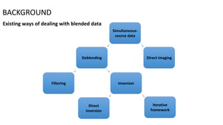
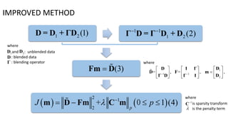
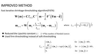
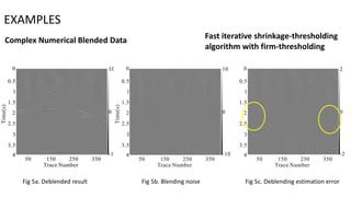
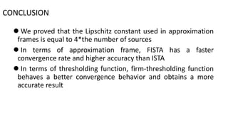
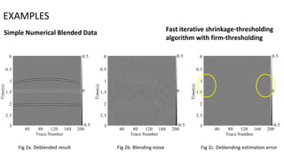
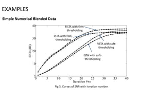
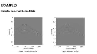
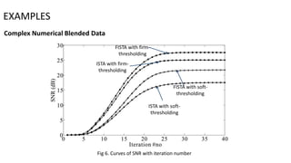
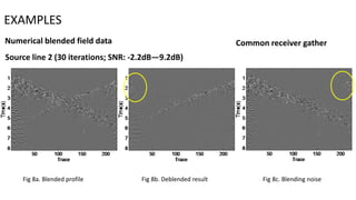
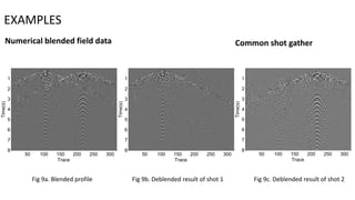
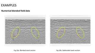
1) The document presents an improved method for deblended simultaneous-source seismic data using a fast iterative shrinkage-thresholding algorithm with firm-thresholding. 2) Numerical examples on both simple and complex blended data models show the new method achieves better signal-to-noise ratio and estimation accuracy compared to other methods. 3) The method is also tested on numerical blended field data with common receiver gathers and common shot gathers, demonstrating noise removal and improved deblended stack sections.

1. BACKGROUND
Simultaneous-source
Ocean Bottom Nodes acquisition
Common receiver gather

2. BACKGROUND
Existing ways of dealing with blended data
Simultaneous-
source data
Direct imagingDeblending
Filtering Inversion
Direct
inversion
Iterative
framework

3. IMPROVED METHOD
1 2 (1)D = D + ΓD 1 1
1 2 (2) 
Γ D = Γ D + D
(3)Fm D 1
1 1
2
= , = , , 
    
     
     
DD I Γ
D F m
DΓ D Γ I
and : unblended data
: blended data
: blending operator
where
where
2D1D
D
Γ
   
2
1
2
+ 1 (4)
p
J p 
   m D Fm C m 0 is sparsity transform
is the penalty term
where
1
C


4. IMPROVED METHOD
   1
,2
2 T
T
L
 
  
    
W m C C m F Fm d
 1 1
1
1
+ k
k k k k
k
t
t
 

 
  
 
m W m m m
Fast iterative shrinkage-thresholding algorithm(FISTA)
   
      
 
,2
, for 4 ,
4
sgn , for 4 ,
4 1
0, for
k k
k k k
k
v v
T v v v
v
 


  


 


      
 

m m
m m m
m
  2
1 1+ 1 4 2k kt t  where
 Reduced the Lipschitz constant :
 Used firm-thresholding instead of soft-thresholding
L =4*the number of blended sourcesL

5. Simple Numerical Blended Data
EXAMPLES
Fig 1a. Unblended profile Fig 1b. Blended profile

6. Simple Numerical Blended Data
EXAMPLES
Fast iterative shrinkage-thresholding
algorithm with firm-thresholding
Fig 2a. Deblended result Fig 2b. Blending noise Fig 2c. Deblending estimation error

7. Simple Numerical Blended Data
EXAMPLES
Fig 3. Curves of SNR with iteration number
ISTA with firm-
thresholding
ISTA with soft-
thresholding
FISTA with soft-
thresholding
FISTA with firm-
thresholding

8. EXAMPLES
Complex Numerical Blended Data
Fig 4a. Unblended profile Fig 4b. Blended profile

9. EXAMPLES
Fast iterative shrinkage-thresholding
algorithm with firm-thresholding
Complex Numerical Blended Data
Fig 5a. Deblended result Fig 5b. Blending noise Fig 5c. Deblending estimation error

10. EXAMPLES
ISTA with firm-
thresholding
ISTA with soft-
thresholding
FISTA with soft-
thresholding
FISTA with firm-
thresholding
Complex Numerical Blended Data
Fig 6. Curves of SNR with iteration number

11. EXAMPLES
Numerical blended field data Common receiver gather
Fig 7a. Blended profile Fig 7b. Deblended result Fig 7c. Blending noise
Source line 1 (30 iterations; SNR: 2.2dB—11.6dB)

12. Common receiver gather
EXAMPLES
Numerical blended field data
Fig 8a. Blended profile Fig 8b. Deblended result Fig 8c. Blending noise
Source line 2 (30 iterations; SNR: -2.2dB—9.2dB)

13. EXAMPLES
Numerical blended field data
Trace
Time(s)
50 100 150 200 250 300
1
2
3
4
5
6
7
8
Trace
Time(s)
50 100 150 200 250 300
1
2
3
4
5
6
7
8
Trace
Time(s)
50 100 150 200 250 300
1
2
3
4
5
6
7
8
Common shot gather
Fig 9a. Blended profile Fig 9b. Deblended result of shot 1 Fig 9c. Deblended result of shot 2

14. EXAMPLES
Numerical blended field data
Fig 10a. Blended stack section Fig 10b. Deblended stack section

15.  We proved that the Lipschitz constant used in approximation
frames is equal to 4*the number of sources
 In terms of approximation frame, FISTA has a faster
convergence rate and higher accuracy than ISTA
 In terms of thresholding function, firm-thresholding function
behaves a better convergence behavior and obtains a more
accurate result
CONCLUSION