This document provides an introduction to genetic algorithms. It begins with a brief overview of genetic algorithms and some of their applications, such as image processing, protein structure prediction, chip layout design, and analysis of time series data. The rest of the document covers the typical components of a genetic algorithm, including an initial population of solutions, a fitness function, operators to combine solutions and introduce mutations, and iteration of these steps over generations. Code implementations and further resources are also discussed.

2. An Introduction
to GeneticAlgo~ithms
for ScientistsandEngineers

3. An Introduction
to GeneticAlgo~ithms
for ScientistsandEngineers

4. An Introduction
to GeneticAlgorithms
for Scientistsand Engineers
DavidA Coley
U n i ~ e ~ i ~of Exeter
World Scientific
Singapore*NewJersey*London4fongKong

5. Published by
World ScientificPublishingCo. Pte.Ltd.
P 0Box 128,FarrerRoad, Singapore912805
USAoffice: Suite fB, 1050Main Street, RiverEdge, NJ 07661
UKoffice: 57 SheltonStreet,CoventGarden,London WC2H 9%
BritishLibraryCataIo~ng-in-PublicatfonData
A cataloguerecord forthisbook is availablefromthe BritishLibrary.
AN INTRODUCTION TO GENETIC ALGORITHMS FOR SCIENTISTS
AND ENGINE~RS
CopyrightQ 1999by World ScientificPublishingCo.Pte.Ltd.
All rightsreserved. Thisbook, orparts thereof,maynot be reproduced in anyform or by any means,
ekctronic or mechanical, includingphofocopying,recording or any informationstorage an&retrieval
systemnow known or to be invented, without writfen~ e ~ i s s i o n ~ o mthe Publisher.
For photocopying of material in this volume, please pay a copying fee through the Copyright
Clearance Center, Inc., 222 RosewoodDrive, Danvers, MA 01923,USA. In this case permissionto
photocopy is not required from the publisher.
ISBN 981-02-3602-6
Thisbook isprintedon acid-free paper.
Printed in Singaporeby Uto-Print

6. In the beginning was the Word
And by the mutationscame the Gene
MA. Arbid
Word
Wore
Gore
Gone
Gene

7. An Introduction
to GeneticAlgo~ithms
for ScientistsandEngineers

8. Tomy parents

9. An Introduction
to GeneticAlgo~ithms
for ScientistsandEngineers

10. ix
PREFACE
Genetic algorithms (GAS) are general search and optimisation algorithms
inspired by processes normally associated with the natural world. The approach
is gaining a growing following in the physical, life, computer and social
sciences and in engineering. Typically those interested in GAScan be placed
into one or more of three rather loose categories:
1. those using such algorithms to help understand some of the processes and
dynamicsof natural evolution;
2. computer scientistsprimarily interestedin understandingand improvingthe
techniques involved in such approaches,or constructingadvanced adaptive
systems;and
3. those with other interests, who are simplyusing GASas a way to help solve
a range of difficult modellingproblems.
This book is designed first and foremost with this last group in mind,
and hence the approach taken is largely practical. Algorithms are presented in
full, and working code (in BASIC, FORTRAN, PASCAL and C) is included
on a floppy disk to help you to get up and running as quickly as possible.
Those wishing to gain a greater insight into the current computer science of
GAS, or into how such algorithms are being used to help answer questions
about natural evolutionary systems, should investigateone or more of the texts
listed in Appendix A.
Although I place myself in the third category, I do find there is
something fascinating about such evolutionary approaches in their own right,
somethingalmost seductive,somethingfun. Why this should be I do not know,
but there is something incredible about the power of the approach that draws
one in and creates a desire to know that little bit more and a wish to try it on
ever harder problems.
All I can say is this: if you have never tried evolutionary inspired
methods before, you should suspend your disbelief, give it a go and enjoy the
ride.
This book has been designed to be usehl to most practising scientists
and engineers (not necessarily academics), whatever their field and however
rusty their mathematicsand programming might be. The text has been set at an
introductory, undergraduate level and the first five chapters could be used as
part of a taught course on search and optimisation. Because most of the
operations and processes used by GAS are found in many other computing

11. X
situations, for example: loops; file access; the sorting of lists; transformations;
random numbers; the systematic adjustment of internal parameters; the use of
multiple runs to produce statistically significant results; and the role of
stochastic errors, it would, with skill, be possible to use the book as part of a
general scientific or engineering computing course. The writing of a GA itself
possibly makes an ideal undergraduate exercise, and its use to solve a real
engineering or scientific problem a good piece of project work. Because the
algorithm naturally separates into a series of smaller algorithms, a GA could
also form the basis of a simple piece of groupprogrammingwork.
Student exercises are included at the end of several of the chapters.
Many of these are computer-basedand designed to encourage an explorationof
the method.
Please email any corrections, comments or questions to the address
below. Any changes to the text or software will be posted at
http:llwww.ex.ac.Wceelga! .
David A. Coley
Physics Department
Universityof Exeter
September 1998
D.A.Coley@exeter.ac.uk
All trademarksare acknowledged as thepropertyof theirrespectiveowners
The Internetand World Wide Webaddresseswere checked as closetopublicationaspossible,
however the locationsand contentsof such sites are subjectto changesoutwiththe control of
the author. The authoralso bearsno responsibilityfor the contentsof thoseweb-pageslisted,
these addressesare givenfor the convenienceand interestof readers only.

12. xi
ACKNOWLEDGEMENTS
As with most books, this one owes its existence to many people. First and
foremostto my wife Helen, who translated my scribblednotes and typed up the
result; but more importantly, for organising the helicopters and ambulances,
and lookingafter my body after I lost one of many argumentswith gravity.
Many colleagues have helped directly with the text, either with the
research, providing material for the text, or reading the drafts; including:
Thorsten Wanschura, Stefan Migowsky, David Carroll, Godfrey Walters,
Dragan Savic, Dominic Mikulin, Andrew Mitchell and Richard Lim of World
Scientific.
A final word of thanks is owed to Mr Lawson, my school science
teacher, whose enthusiasmand teaching first openedmy eyes to the wondersof
the physical and natural world and the possibilitiesof science.

13. An Introduction
to GeneticAlgo~ithms
for ScientistsandEngineers

14. xiii
NOTATION
Concatenation,e.g. 00 G3 If = 0011
A c~mosome,stringor structure.
The form of the chromosome, string or structure at the global
optimum.
Fitnessscalingconstant.
Defininglength of a schema.
Fitness.
The shared fitness.
Fitnessat the global optimum.
Theaveragepopulationfitness.
The fitnessof the elitemember.
The minimum fitness required for a solution to be defined as
acceptable, e.g. the lower boundary of the fitness fiker when
huntingfor a seriesof approximatesolutions.
Theoff-linesystemperformance.
Theon-line systemperformance.
Sum of the fitness of all population members in the current
generation.
The standard deviation of the population fitness in the current
generation.
Generation.
Maximumnumber of generations.
Typicallyusedto indicatean individualwithin the population.
Lengthof thebinary stringused to representa singleunknown.
Total string(or c~omosome)length.
Numberof unknown parameters in the problem.
Find the maximumof functionf.
Populationsize.
Order of a schema.
Crossoverprobability.
Mutationprobability.
Randomdecimalnumber.
Unknown parameter (typically real-valued), the optimum value of
whichthe GA is beingused to discover.
Fitness-propo~ional{roulettewheel) selection.
Randomdecimal number in the range 0 to +l.
Randomdecimal number in the range -1to +1.

15. xiv
R C
Q
P
9"
.r
r
I
Q
101
Random number used to decide if an individual will undergo
crossover.
Random number indicatingthe crossoverposition.
Maximumpossible value of the unknown r.
Minimumpossible value of the unknown r.
Random number used to decide if an individual will be selected to
go forward to the next generation.
Schema.
Sharingfunction for individual i.
Variable;c.f. x, which indicatesmultiplication.
Unknown parameter expressedas a base ten integer.
Maximumvalue of an unknown expressedas a base ten integer.
Minimum value of an unknown expressedas a base ten integer.
Elitism; equals 1if elitism is being applied, 0 if not.
Genotypic similarity between the elite member and the rest of the
population.
Sharingvalue between individualsi andj.
The number of optima in a multimodal function.
Actual number of trials in the next generation.
Number of trials in the next generation an individual of average
fitness might receive.
Number of trials in the next generation the elite member will
receive.
Expectednumber of trials in the next generation.
Expected number of trials in the next generation the elite member
might receive.
The take-overtime, i.e., the number of generationstaken by the elite
member to dominate the population.
Selectionmechanism.
Problem objective function (the maximum or minimum value of
which is being sought), fitness will typically be a very simple
function of Q.
Number of instances of a particular schema within a population.
The number of multiple runs carried out to reduce the effects of
stochasticerrors.
Example of a binary number; c.f. 101,a decimal number.

16. xv
CONTENTS
Chapter 1 Introduction
1.1
1.2 Search Spaces
1.3 GeneticAlgorithms
1.4 An Example
1.5 Summary
1.6 Exercies
SomeApplications of GeneticAlgorithms
Chapter 2 Improvingthe Algorithm
2.1
2.2 Robustness
2.3 Non-integer Unknowns
2.4 Multiparameter Problems
2.5 Mutation
2.6 Selection
2.7 Elitism
2.8 Crossover
2.9 Initialisation
2.10 The Little Genetic Algorithm
2.11 Other EvolutionaryApproaches
2.12 Summary
2.13 Exercises
Comparison of Biological andGATerminology
Chapter 3 Foundations
3.1 HistoricalTest Functions
3.2 SchemaTheory
3.3 SchemaProcessing
3.4 OtherTheoreticalApproaches
3.5 Summary
3.6 Exercises
Chapter4 Advanced Operators
4.1 CombinatorialOptimisation
4.2
4.3 Constraints
4.4 MulticriteriaOptimisation
4.5 Hybrid Algorithms
4.6 AlternativeSelectionMethods
Locating AlternativeSolutionsUsing Niches and Species
1
2
3
10
11
15
16
17
17
18
19
22
22
23
25
25
26
26
32
33
33
35
36
46
53
57
58
58
59
59
64
72
73
76
78

17. xvi
4.7
4.8
4.9
4.10
4.11
4.12
4.13
4.14
Alternative CrossoverMethods
Considerationsof Speed
Other Encodings
Meta GAS
Mutation
Parallel Genetic Algorithms
Summary
Exercises
Chapter 5 Writing a GeneticAlgorithm
Chapter 6 Applicationsof GeneticAlgorithms
6.1
6.2
6.3
6.4
6.5
6.6
6.7
6.8
Appendix A
Appendix I3
References
Index
ImageRegistration
RecursivePre~ictionof Natural Light Levels
Water Network Design
Ground-StateEnergy of the fJ Spin Glass
Estimation of the Optical Parameters of Liquid Crystals
Design of Energy-Efficient Buildings
Human Judgement as the FitnessFunction
Multi-Obj~tiveNetwork Rehabili~tionby Messy GA
Resources and Paper-BasedResources
CompleteListing of LGADOS.BAS
83
84
85
89
89
90
91
91
93
113
117
123
131
139
144
157
168
176
187
189
205
225

18. 1
CHAPTER1
INTRODUCTION
Genetic algorithms (GAS) are numerical optimisation algorithms inspired by
both natural selection and natural genetics. The method is a general one,
capable of being applied to an extremelywide range of problems. Unlike some
approaches,their promise has rarely been over-sold and they are being used to
help solve practical problems on a daily basis. The algorithms are simple to
understand and the required computer code easy to write. Although there is a
growing number of disciples of GAS, the technique has never attracted the
attention that, for example, artificial neural networks have. Why this should be
is difficult to say. It is certainlynot because of any inherent limits or for lack of
a powerfid metaphor. What could be more inspiringthan generalisingthe ideas
of Darwin and others to help solve other real-world problems? The conceptthat
evolution, starting from not much more than a chemical "mess", generated the
(unfortunatelyvanishing) bio-diversity we see around us today is a powerful, if
not awe-inspiring,paradigm for solvingany complexproblem.
In many ways the thought of extending the concept of natural selection
and natural geneticsto other problems is such an obvious one that one might be
left wondering why it was not tried earlier. In fact it was. From the very
beginning, computer scientists have had visions of systems that mimicked one
or more of the attributes of life. The idea of using a population of solutions to
solve practical engineeringoptimisationproblems was consideredseveraltimes
during the 1950's and 1960's. However, GASwere in essence invented by one
man-John Holland-in the 1960's. His reasons for developing such
algorithms went far beyond the type of problem solving with which this text is
concerned. His 1975 book, Adaptation in Natural and Artwcial Systems
[H075] (recently re-issued with additions) is particularly worth reading for its
visionary approach. More recently others, for example De Jong, in a paper
entitled GeneticAlgorithms are NOT Function Optimizers [DE93], have been
keen to remind us that GASare potentially far more than just a robust method
for estimating a series of unknown parameters within a model of a physical

19. system. However in the context of this text, it is this robustness across many
differentpractical optimisationproblemsthat concernsus most.
So what is a GA? A typical algorithmmight consist of the following:
1. a number, or population,of guessesof the solutionto the problem;
2. a way of calculating how good or bad the individual solutions within the
populationare;
3. a method for mixing fragments of the better solutions to form new, on
averageeven better solutions;and
4. a mutation operator to avoid permanent loss of diversity within the
solutions.
With typically so few components, it is possible to start to get the idea
ofjust how simple it is to produce a GA to solve a specific problem. There are
no complex mathematics, or torturous, impenetrable algorithms. However, the
downside of this is that there are few hard and fast rules to what exactly a GA
is.
Before proceeding further and discussing the various ways in which
GAShave been constructed, a sample of the range of the problems to which
they have been successfullyapplied will be presented, and an indication given
of what is meant by the phrase “searchand optimisation”.
1.1 SOME APPLICATIONSOF GENETICALGORITHMS
Why attempt to use a GA rather than a more traditional method? One
answer to this is simply that GAS have proved themselves capable of solving
many large complex problems where other methods have experienced
difficulties. Examples are large-scale combinatorial optimisation problems
(such as gas pipe layouts) and real-valued parameterestimations (such as image
registrations) within complex search spaces riddled with many local optima, It
is this ability to tackle search spaces with many local optima that is one of the
main reasons for an increasing number of scientists and engineers using such
algorithms.
Amongst the many practical problems and areas to which GAS have
been successfullyappliedare:

20. 3
imageprocessing [CH97,KA97];
prediction of three dimensionalprotein structuresfSC921;
VLSI (verylarge scaleintegration)electronicchip layouts [COH91,ES94];
lasertechnology[CA96a,CA96b];
medicine [YA98];
spacecrafttrajectories[RA96];
analysisof time series [MA96,ME92,ME92a,PA90];
solid-statephysics [S~94,WA96];
aeronautics[BR89,YA95];
liquidcrystals[MIK97];
robotics [ZA97,p161-2021;
water networks [HA97,SA97];
evolvingcellularautomatonrules [PA88,MI93,MI94a];
the ~hitectura~aspectsof buildingdesign [MIG95,FU93];
the automaticevolutionof computer sohare [KO91,K092,K094];
aesthetics[CO97a];
jobshop scheduling[KO95,NA9l,YA95];
facial recognition [CA91];
trainingand designingartificialintelligencesystemssuch as artificialneural
networks [ZA97,p99-117,WH92, ~90,~94,CH90];and
control "09 1,CH96,C097].
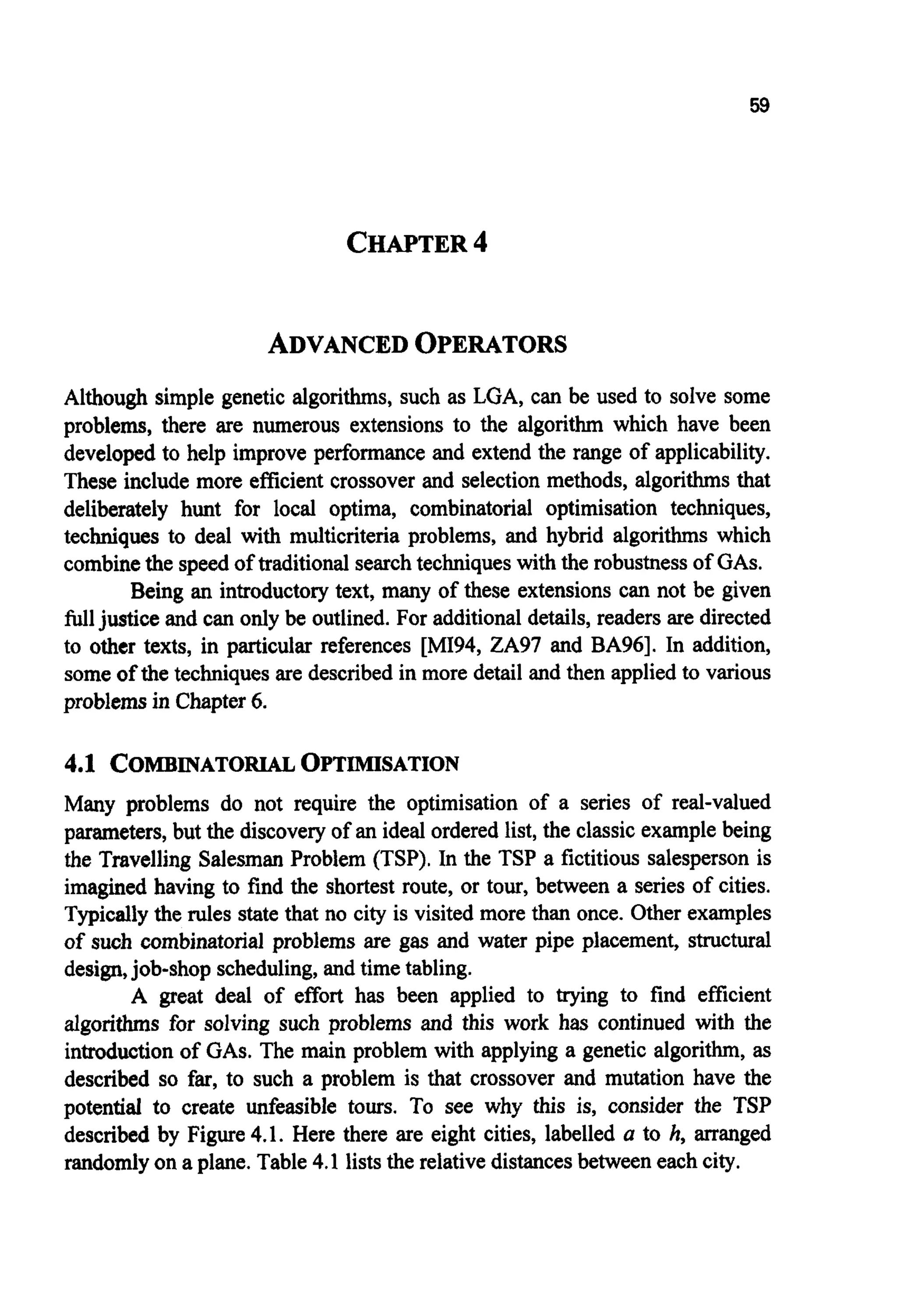
1.2 SEARCHSPACES
In a numerical search or optimisation problem, a list, quite possibly of infinite
length, of possible solutions is being searched in order to locate the solution
that best describesthe problem at hand. An examplemight be trying to find the
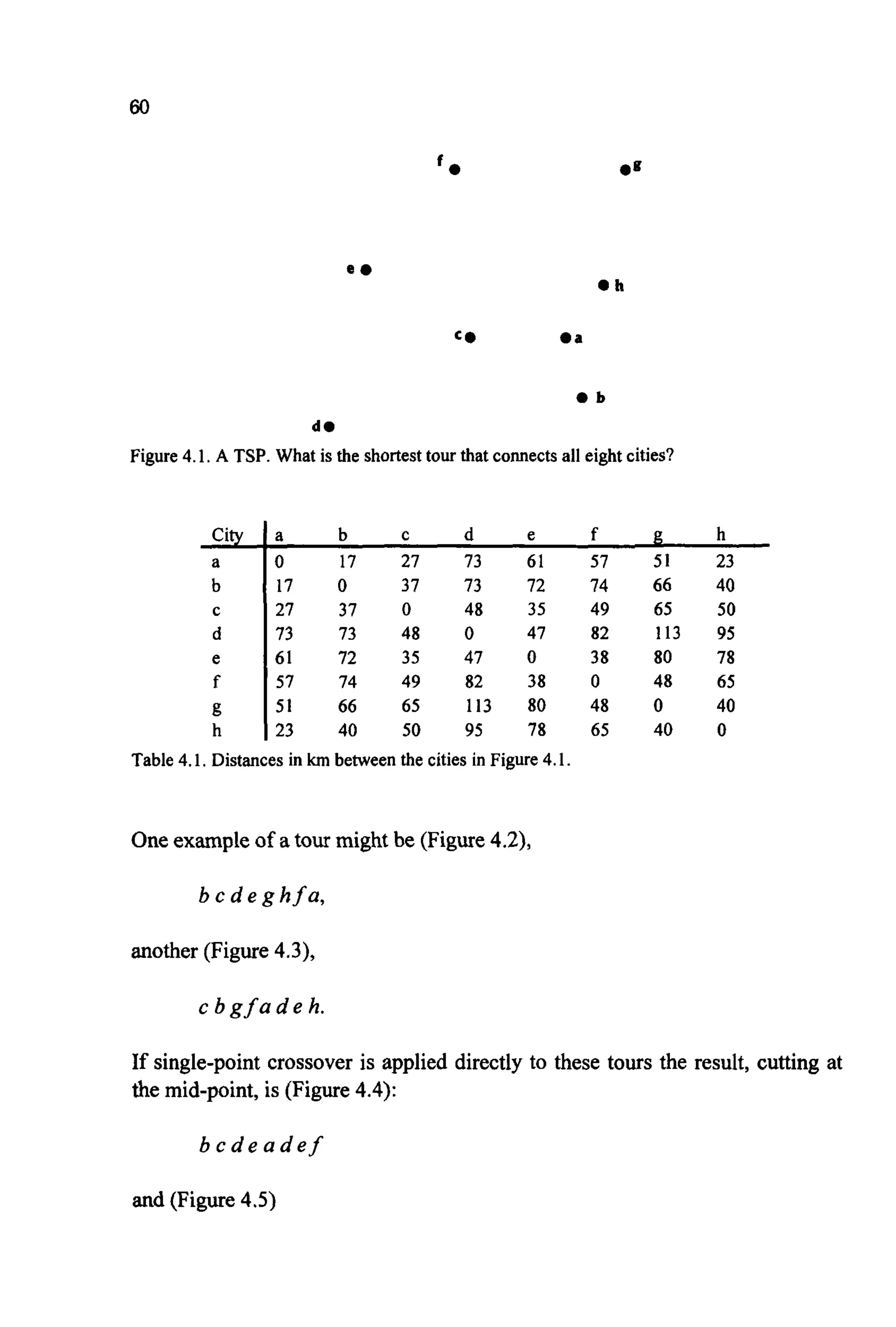
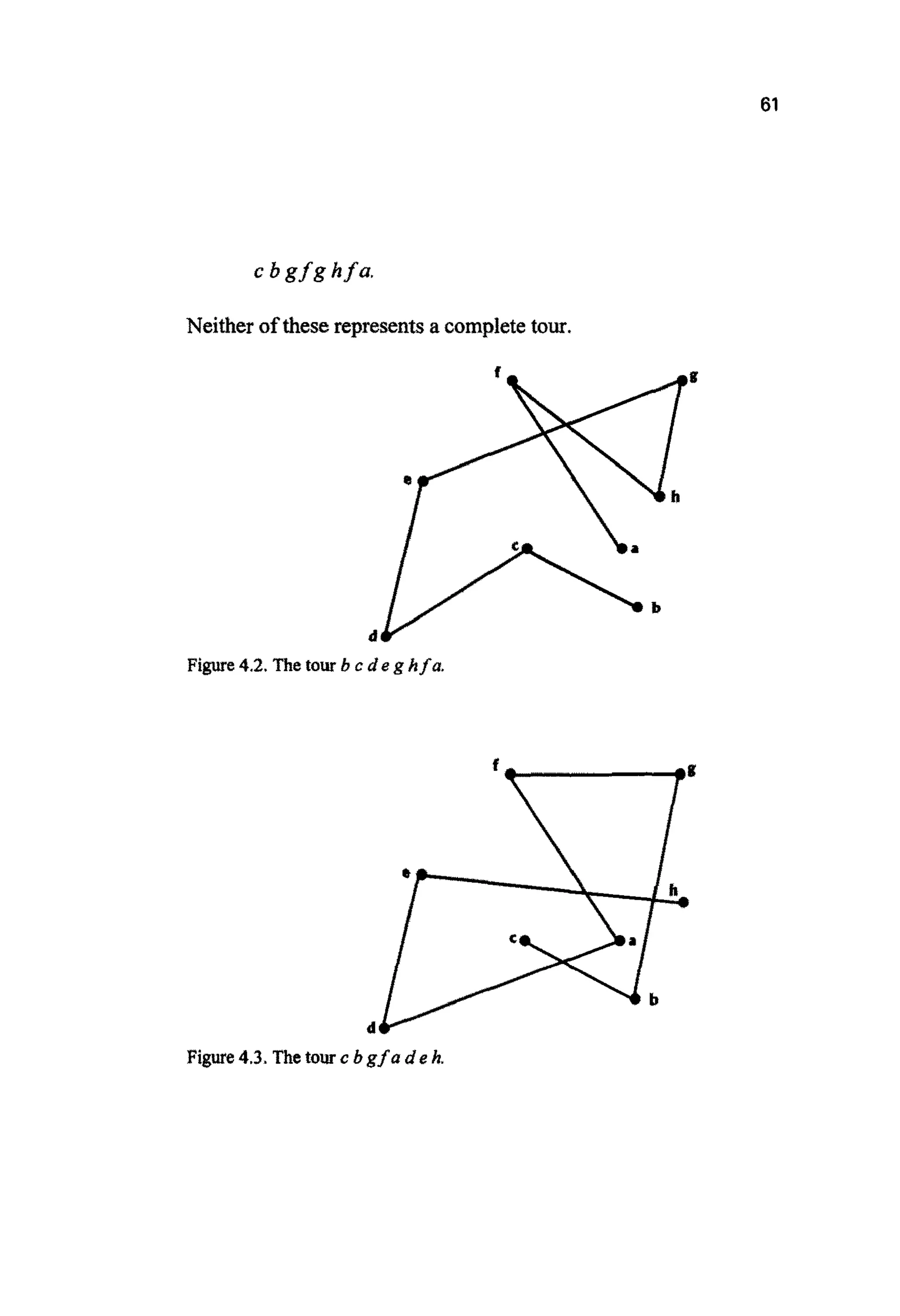
best values for a set of adjustableparameters (or variables)that, when included
in a ~ ~ e ~ t i c a lmodel, maximisethe lift generatedby an aeroplane's wing. If
there were only two of these adjustableparameters, a and b, one could try a
large number of combinations, calculate the lift generated by each design and
produce a surface plot with a, b and l@ plotted on the x-, y- and z-axis
respectively (Figure 1.0). Such a plot is a representation of the problem's
searchspace. For more complexproblems, with more than two unknowns, the
situation becomes harder to visualise. However, the concept of a search space
is still valid as long as some measure of distance between solutions can be
defined and each solution can be assigned a measure of success, orjtness,
within the problem. Better performing,or fitter, solutionswill then occupy the

21. 4
peaks within the search space (or fitness landscape [WR31])and poorer
solutions the valleys.
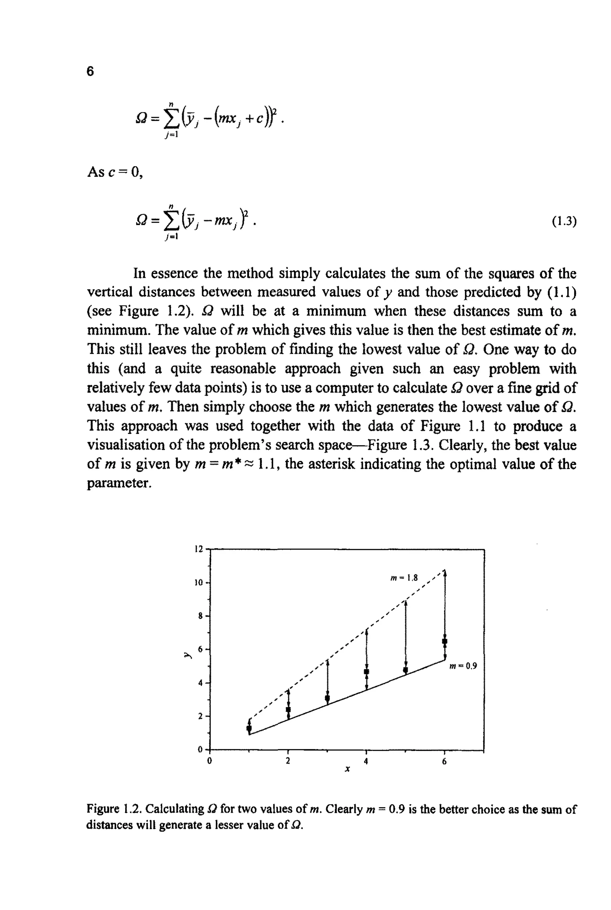
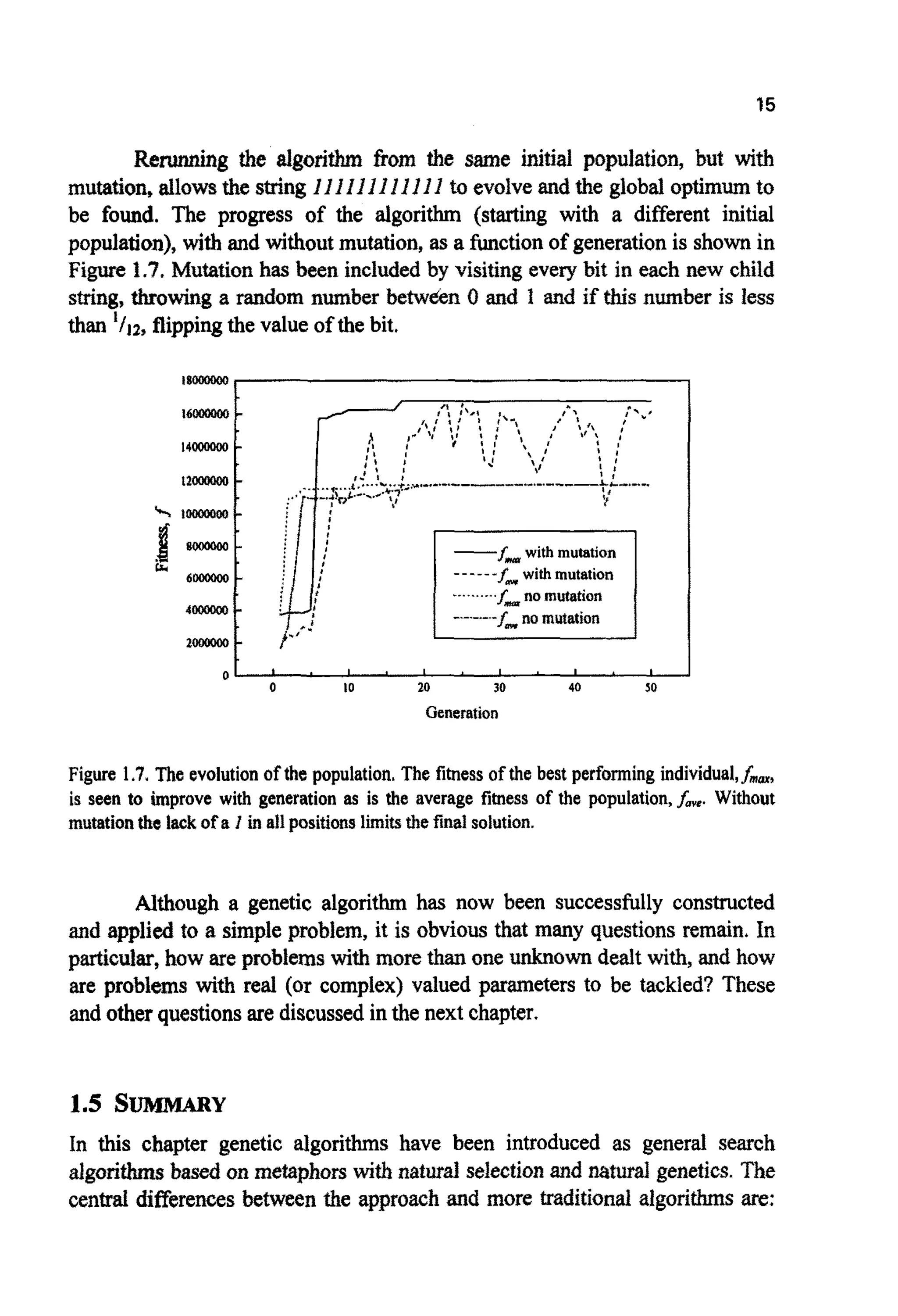
Figure 1.0. A simple search space or “fitness landscape”.The lift generated by the wing is a
functionof the two adjustableparametersa and b. Thosecombinationswhich generatemore lift
are assigned a higher fitness. Typically, the desire is to find the combinationof the adjustable
parameters that givesthe highest fitness.
Such spaces or landscapes can be of surprisingly complex topography.
Even for simple problems, there can be numerous peaks of varying heights,
separated from each other by valleys on all scales. The highest peak is usually
referred to as the global m ~ ~ m ~ ~or global ~p~imum,the lesser peaks as local
maxima or local optima. For most search problems, the goal is the accurate
identification of the global optimum, but this need not be so. In some
situations, for examplereal-time control, the identificationof any point above a
certain value of fitness might be acceptable. For other problems, for example,
in architectural design, the identification of a large number of highly fit, yet
distant and therefore distinct, solutions (designs)might be required.
To see why many traditional algorithms can encounter difficulties,
when searching such spaces for the global optimum, requires an understanding
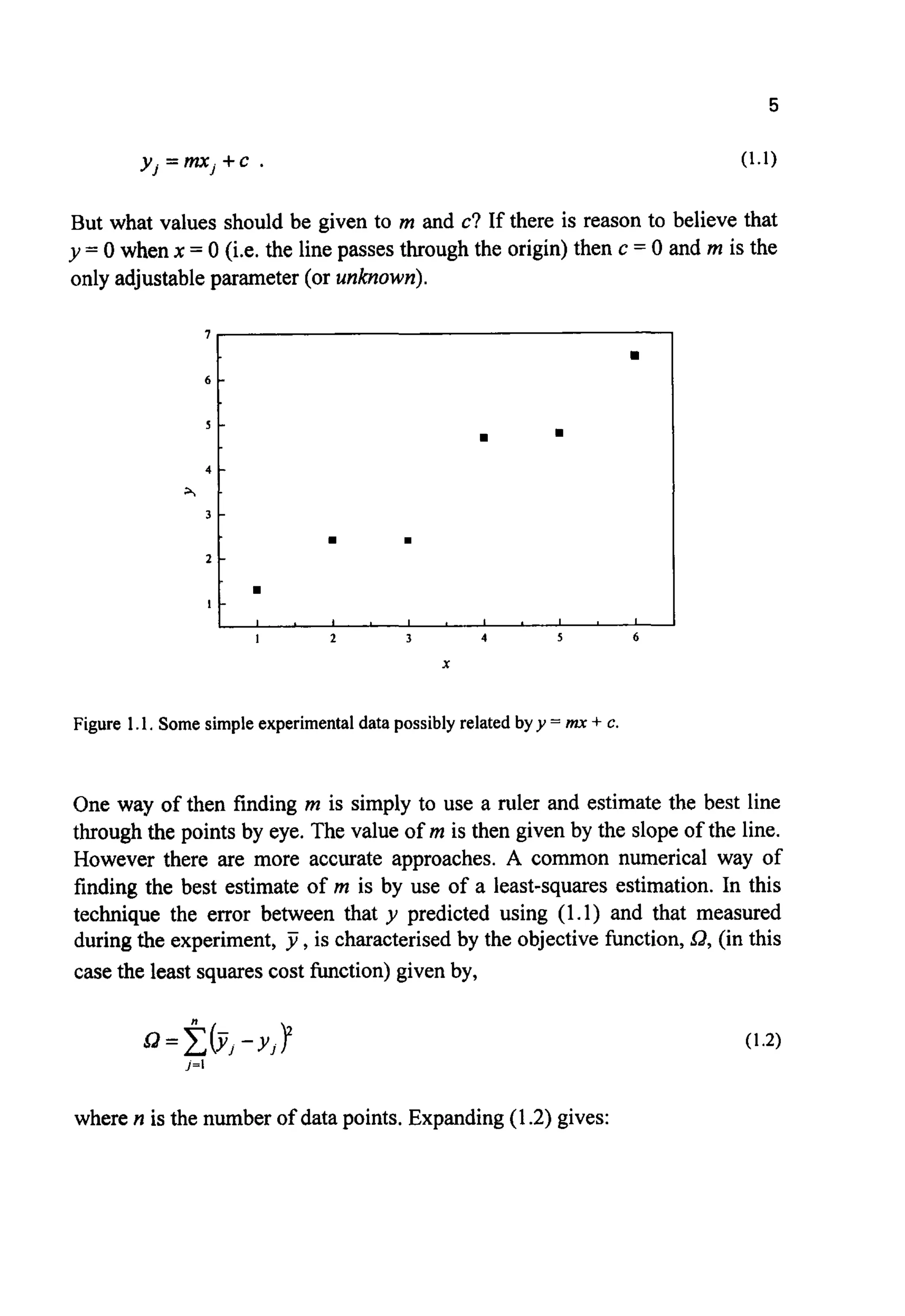
of how the features within spaces are formed. Consider the experimental data
shown in Figure 1.1, where measurementsof a dependent variabley have been
made at various pointsj of the independent variable x. Clearly there is some
evidencethat x andy might be related through:

22. 5
1
6 -
s -
4 -
A -
3 -
2 -
I -
y .=m.+ c . (1.1)J J
rn
I . 1 1 1 1 1 . I I I
But what values should be given to m and c? If there is reason to believe that
y = 0 when x = 0 (i.e. the line passes through the origin) then c = 0 and m is the
only adjustable parameter (or unknown).
Figure 1.1. Some simple experimental data possibly related by y = mx + c.
One way of then finding m is simply to use a ruler and estimate the best line
through the points by eye. The value of m is then given by the slope of the line.
However there are more accurate approaches. A common numerical way of
finding the best estimate of m is by use of a least-squares estimation. In this
technique the error between that y predicted using (1.1) and that measured
during the experiment, J ,is characterisedby the objective function, 0,(in this
case the least squares cost function) given by,
where n is the number of data points. Expanding(1.2) gives:

23. 6
Asc=O,
In essence the method simply calculates the sum of the squares of the
vertical distances between measured values of y and those predicted by (1.1)
(see Figure 1.2). Q will be at a minimum when these distances sum to a
minimum. The value of m which gives this value is then the best estimate of rn.
This still leaves the problem of finding the lowest value of 9.One way to do
this (and a quite reasonable approach given such an easy problem with
relativelyfew data points) is to use a computerto cakulate Q over a fme grid of
values of m.Then simply choose the m which generates the lowest value of 4.
This approach was used together with the data of Figure 1.1 to produce a
visualisation of the problem’s search space-Figure 1.3.Clearly, the best value
of m is given by m = m *=: 1.1, the asterisk indicating the optimal value of the
parameter.
12 ,
I0 -
8-
A 6 -
4 -
2 -
,
0 2 4 6
X
Figure 1.2.Calculating9for two values of m. Clearly m = 0.9 is the better choice as the sum of
distanceswill generate a lesser value of Q.

24. 7
m
Figure 1.3. A simple search space, created from the data of Figure 1.1, Equation (1.3) and a
large number of guesses of the value of m. This is an example of a minimisation problem,
where the optimumis located atthe lowestpoint.
This approach, of estimating an unknown parameter, or parameters, by
simply solvingthe problem for a very large number of values of the unknowns
is called an enumerative search. It is only really usehl if there are relatively
few unknownparameters and one can estimateL? rapidly. As an example why
such an approach can quickly run into problems of scale, consider the
following. A problem in which there are ten unknowns, each of which are
required to an accuracy of one percent, will require 10010, or 1x1020,
estimations. If the computer can make 1000 estimationsper second, then the
answer will take over 3x109years to emerge, Giventhat ten is not a very large
number of unknowns, one percent not a very demanding level of accuracyand
onet h o u s ~ devaluationsper secondmore than respectable for ~~y problems,
clearlythere is a need to find a better approach.
Returningto Figure 1.3, a brief consideration of the shape of the curve
suggestsanother approach: guesstwo possible values of m,labelled ml and m2
(see Figure 1.4), then if Q(m4 > Sa(ml),make the next guess at some point m3
where 1113 =m2 +6, or else head the other way. Given some suitable,dynamic,
way of adjustingthe value of 6, the method will rapidlyhome in on m*.

25. 8
0.0 0 s I.o 1.5 2.0
m
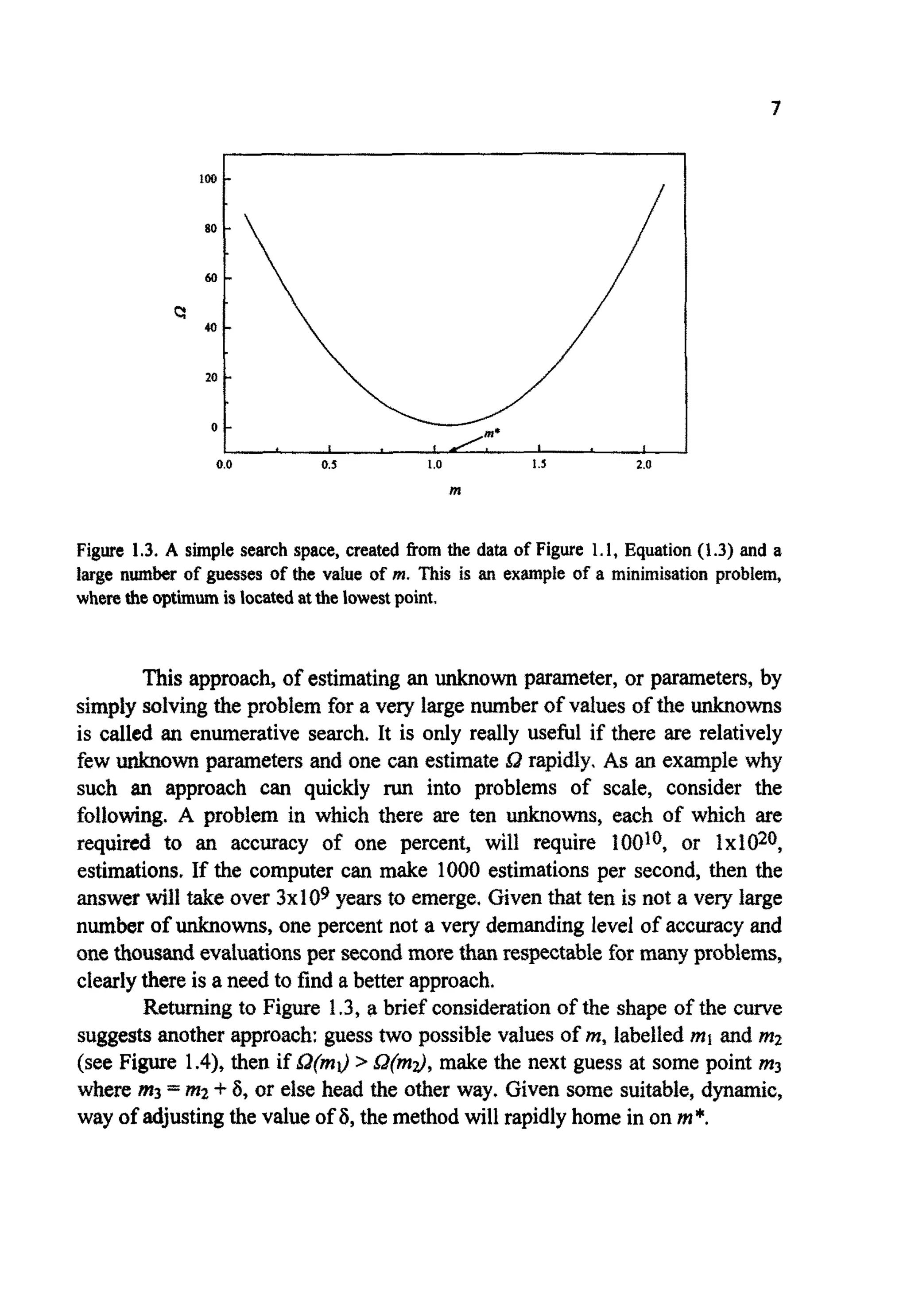
Figure 1.4.A simple, yet effective, method of locating m*. 6 is reduced as the minimum is
approached.
Such an approach is described as a direct search (because it does not
make use of derivatives or other information).The problem illustrated is one of
minimisation. If 1lQ were plotted, the problem would have been transformed
into one of maximisation and the desire would been to locate the top ofthe hill.
U n f o ~ ~ a t e l y ,such methods cannot be universally applied. Given a
different problem, still with a single adjustable parameter, a, might take the
form shown in Figure 1.5.
If either the direct search algorithm outlined above or a simple calculus
based approach is used, the final estimate of a will depend on where in the
search space the algorithm was started. Making the initial guess at a =u2, will
indeed lead to the correct (or global) minimum, a*.However, if a = a] is used
then only a** will be reached (a local minimum).

26. 9
4
3
c
2
I
I 2 3 4 5
a
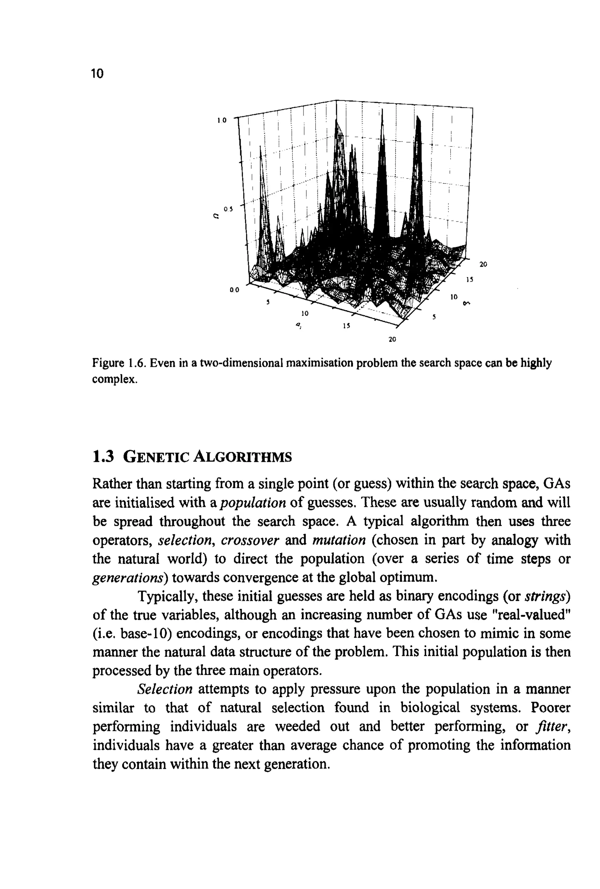
Figure 1.5. A morecomplexon~dimensiona1search spacewith both aglobalanda local
minimum.
This highlights a serious problem. If the results produced by a search
algorithm depend on the startingpoint, then there will be little confidence in
the answers generated. In the case illustrated, one way around this problem
would be to start the problem from a seriesof points and then assume that the
true global mi^^ lies at the lowest minimum identified.This is a frequently
adopted strategy. Unfortunately Figure 1.5 represents a very simple search
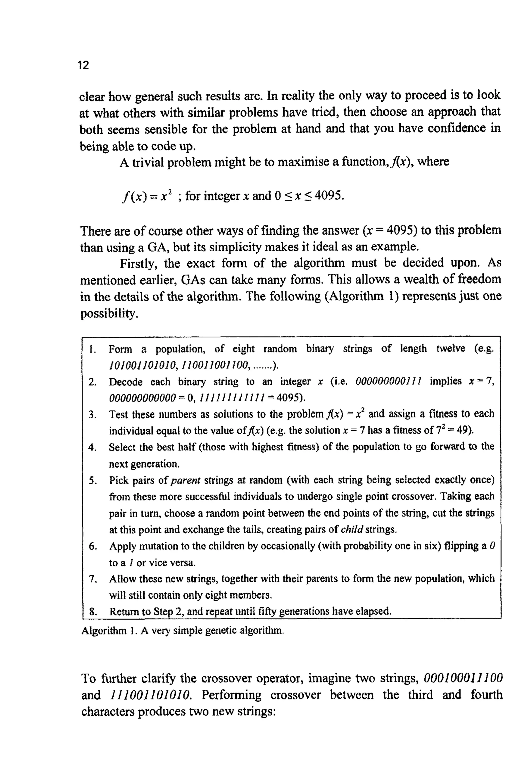
space. In a more complex space (such as Figure 1.6) there may be very many
local optimaandthe approachbecomeswealistic.
So, how are complex spaces to be tackled? Many possible approaches
have been suggestedand found favour, suchas random searchesand simulated
annealing [DA87]. Some of the most successful and robust have proved to be
random searches directed by analogies with natural selection and natural
genetics-genetic algorithms,

27. 10
20
Figure 1.6.Even in a two-dimensionalmaximisation problem the search space can be highly
complex.
1.3 GENETICALGORITHMS
Rather than starting from a single point (or guess) within the search space, GAS
are initialised with apopulution of guesses. These are usually random and will
be spread throughout the search space. A typical algorithm then uses three
operators, selection, crossover and mutation (chosen in part by analogy with
the natural world) to direct the population (over a series of time steps or
generations) towards convergenceat the global optimum.
Typically,these initial guesses are held as binary encodings (or strings)
of the true variables, although an increasing number of GAS use "real-valued"
(i.e. base-10) encodings, or encodings that have been chosen to mimic in some
manner the natural data structure of the problem. This initial population is then
processed by the three main operators.
Selection attempts to apply pressure upon the population in a manner
similar to that of natural selection found in biological systems. Poorer
performing individuals are weeded out and better performing, or fitter,
individuals have a greater than average chance of promoting the information
they contain within the next generation.

28. 11
Crossoverallowssolutionsto exchange informationin a way similarto
that used by a natural organism undergoing sexual reproduction. One method
(termed single point crossover) is to choose pairs of individualspromoted by
the selection operator, randomly choose a single locus (point) within the binary
strings and swap all the information (digits) to the right of this locus between
thetwo individuals.
~ # ~ a ~ o ~is used to randomly change (flip) the value of single bits
within individ~lstrings.~ u ~ t i o nis typical~yused very sparingly.
After selection,crossoverand mutation have been applied to the initial
population, a new population will have been formed and the generational
counter is increased by one. This process of selection, crossover and mutation
is continued until a fixed number of generationshave elapsed or some form of
convergencecriterionhas been met.
On a first encounterit is fw from obvious that this process is everlikely
to discoverthe global optimum,let aloneformthe basis of a general and highly
effmtive search algorithm. However, the application of the technique to
numerous problems across a wide diversity of fields has shown that it does
exactlythis. The ultimate proof of the utility of the approachpossibly lies with
the demonstratedsuccessof life on earth.
1.4 ANEXAMPLE
There are many things that have to be decided upon before applying a GA to a
p ~ c ~ ~problem, including:
the method of encodingthe unknownparameters(as binary strings, base-10
numbers,etc.);
how to exchangeinformationcontainedbetween the stringsor encodings;
the population size-typical values are in the range 20 to 1000, but can be
smalleror much larger;
how toapply the conceptof mutationto the representation;and
the terminationcriterion.
Many papers have been written discussing the advantages of one
encoding over another; or how, for a particular problem, the population size
might be chosen [GO89b]; about the difference in performance of various
exchange mechanismsand on whether mutation rates ought to be high or low,
However, these papers have naturally concerned themselves with computer
experiments, using a small number of simple test hctions, and it is often not

29. 12
clear how general such results are. In reality the only way to proceed is to look
at what others with similar problems have tried, then choose an approach that
both seems sensible for the problem at hand and that you have confidence in
being able to code up.
A trivial problem might be to maximise a function,f(x), where
f ( x ) =x2 ;for integerx and 0 5x 54095.
There are of course other ways of finding the answer (x =4095)to this problem
than using a GA, but its simplicitymakes it ideal as an example.
Firstly, the exact form of the algorithm must be decided upon. As
mentioned earlier, GAScan take many forms. This allows a wealth of Ereedom
in the details of the algorithm. The following (Algorithm 1) representsjust one
possibility.
Form a population, of eight random binary strings of length twelve (e.g.
Decode each binary string to an integer x (i.e. OOOOOOOOOIll implies x = 7,
000000000000= 0,I IIfIIf III l l = 4095).
Test these numbers as solutions to the problem Ax) = x2 and assign a fitness to each
individual equal to the value ofAx) (e.g. the solution x = 7 has a fitness of 72= 49).
Select the best half (those with highest fitness) of the population to go forward to the
next generation.
Pick pairs of parent strings at random (with each string being selected exactly once)
from these more successful individuals to undergo single point crossover. Taking each
pair in turn, choose a random point between the end points of the string, cut the strings
at this point and exchange the tails, creating pairs of childstrings.
Apply mutation to the children by occasionally (with probability one in six) flipping a 0
to a I or vice versa.
Allow these new strings, together with their parents to form the new population, which
will still contain only eight members.
101001ioiaio, ifooffaofioa,.......1.
1 8.
A l g o r i t ~1. A very simple genetic a l g o r i t ~ .
Return to Step 2, and repeat until fiegenerations have elapsed.
To further clarify the crossover operator, imagine two strings, 000100011I00
and I11001I01010. Performing crossover between the third and fourth
charactersproduces two new strings:

30. 13
parents children
000/100011100 000001101010
111/00]101010 111100011100
It is this process of crossover which is responsible for much of the power of
geneticalgorithms.
Returning to the example, let the initial populationbe:
population
member
1
2
3
4
5
6
7
8
string
110101100100
010100010111
101111101110
010100001100
011101011101
loIIolooIooI
101011011010
010011010101
X
3428
1303
3054
1292
1885
2889
2778
1237
fitness
11751184
1697809
9326916
1669264
3553225
8346321
7717284
1530169
Population members 1, 3, 6 and 7 have the highest fitness. Deleting those four
with the least fitness provides a temporaryreduced populationready to undergo
crossover:
temp. pop. string X fitness
member
1 110101100100 3428 11751184
2 IolIlllolIIo 3054 9326916
3 I01101001001 2889 8346321
4 10I0110ll010 2778 7717284
Pairs of strings are now chosen at random (each exactly once): 1 is
paired with 2, 3 with 4.Selecting, again at random, a crossover point for each
pair of strings (marked by a 0, four new children are formed and the new
population, consisting of parents and offspring only, becomes (note that
mutation is being ignored at present):

31. 14
popuiation
member
I
2
3
4
5
6
7
8
string
11/0101100100
IO/I I I II01110
101l ~ ~ ~ o o l o o l
10l01l/011010
II I I I1101I10
I OOIOII00100
loiioiolloio
10~01l001001
X
3428
3054
2778
4078
2404
2906
276I
2889
fitness
11751184
9326916
834632I
7717284
16630084
5779216
8444836
7623121
The initial population had an average fitness&, of 5065797 and the
fittest individual had a fitness,f , ,of 11751184. In the second ge~eration,
these have risen to: faye = 8402107 and fmm = 16630084. The next temporary
populationbecomes:
temp. pop. string X fitness
member
1 IIOlO~100100 3428 11751184
2 10111110I110 3054 9326916
3 101~01011010 2906 8444836
4 IlIlfllOlllO 4078 I6630084
This temporary population does not contain a I as the last digit in any of the
strings(whereasthe initialpopulationdid). This impliesthat no stsing fromthis
moment on can contain such a digit and the maximum value that can evolve
will be 1I III III l l IO-afIer which point this string will reproduce so as to
dominate the population. This domination of the population by a single sub-
optimal string gives a first indicationof why mutationmight be important. Any
further populations will only contain the same, identical string. This is because
the crossover operator can only swap bits between strings, not introduce any
new information. Mutationcan thus be seen in part as an operatorchargedwith
maintaining the genetic diversity of the population by preserving the diversity
embodied in the initial generation. (For a discussion of the relative benefits of
mutationand crossover, see [SP93a].)
The inclusion of mutation allows the population to leapfrog over this
sticking point. It is worth reiterating that the initial population did include a 1
in all positions. Thus the mutation operator is not necessarily inventing new
information but simply working as an insurance policy against premature loss
of geneticinformation.

32. 15
R e ~ gthe algorithm from the Same initial population, but with
mutation, allowsthe string ZIZZIZI1I J IZ to evolveand the global optimumto
be found. The progress of the algorithm (starting with a different initial
population), withand without mutation, as a functionof generationis shownin
Figure 1.7, Mutation has been included by visiting every bit in each new child
string, throwing a random number betwden 0 and f and if this number is less
than ' / j ~ ,flippingthe value of the bit.
18000000,
-fm with mutation
------f,withmutation
..........f,, no mutation
2000000 -
0 - ' " I ' I ' ' 1 '
0 10 20 30 40 $0
Generation
Figure 1.7.The evolution of the population.The fitness of the best performingindividual,fnm,
is seen to improve with generation as is the average fitness of the population,fme. Without
mutationthe lack of a I in all positions limitsthefinalsolution.
Although a genetic algorithm has now been successfully constructed
and applied to a simple problem, it is obviousthat many questions remain. In
particular, how are problems withrnorethan one unknown dealt with,and how
are problems with real (or complex) valued parameters to be tackled? These
and otherquestionsare discussedin the next chapter.
1.5 SUMMARY
In this chapter genetic algorithms have been introduced as general search
algorithmsbased on metaphors with natural selectionand natural genetics. The
central differencesbetween the approach and more traditional algorithmsare:

33. 16
the manipulation of a population of solutions in parallel, rather than the
sequential adjustment of a single solution; the use of encoded representations
of the solutions, rather than the solutions themselves; and the use of a series of
stochastic(i.e. random based) operators.
The approach has been shown to be successful over a growing range of
difficult problems. Much of this proven utility arises from the way the
population navigates its way around complex search spaces (or jtness
landscapes) so as to avoid entrapmentby local optima.
The three central operators behind the method are selection, crossover
and mutation. Using these operators a very simple GA has been constructed
(Algorithm 1) and applied to a trivial problem. In the next chapter these
operators will be combined once more, but in a form capable of tackling more
difficult problems.
1.6 EXERCISES
1. Given a string of length ten, what is the greatest value of an unknown
Algorithm 1 can search for?
2. What is the resolution of Algorithm 1 when working with a string length of
thirty?
3. Given a string length of 20 and a probability of mutation of '/20 per bit,
what is the probability that a string will emerge from the mutation operator
unscathed?
4. Implement Algorithm 1 on a computer and adapt it to find the value of x
that maximises sin4(x), 0 Ix 5'R to an accuracy of at least one part in a
million (Use a population size of fifty and a mutation rate of
l/(twice the string length).) This will require finding a transformation
between the binary strings and x such that 000...000 implies x = 0 and
I11...III impliesx = 'R.
5. Experiment with your program and the problem of Question 4 by
estimating the average number of evaluations of sin4(x)required to locate
the maximum; (a) as a function of the population size, (b) with, and
without, the use of crossover. (Use a mutation rate of
l/(twice the string length).)

34. 17
CHAPTER2
IMPROVING THE ALGORITHM
Althoughthe examplepresented in Chapter 1 was useful, it left many questions
unanswered. The most pressing of these are:
0 How will the algorithm perform across a wider range of problems?
0 How are non-integer unknowns tackled?
0 How are problems of more than one unknowndealt with?
0 Are there better ways to define the selection operator that distinguishes
between good and very good solutions?
Following the approach taken by Goldberg [GO89], an attempt will be
made to answer these questions by slowly developing the knowledge required
to produce a practical genetic algorithm together with the necessary computer
code. The algorithmand code go by the name Little GeneticAlgorithm or LGA.
Goldberg introduced an algorithm and PASCAL code called the Simple
Genetic Algorithm, or SGA. LGA shares much in common with SGA, but also
contains several differences.LGA is also similar to algorithmsused by several
other authorsand researchers.
Before the first of the above questions can be answered, some of the
terminology used in the chapter needs clarifying, and in particular, its relation
to terms used in the life sciences.
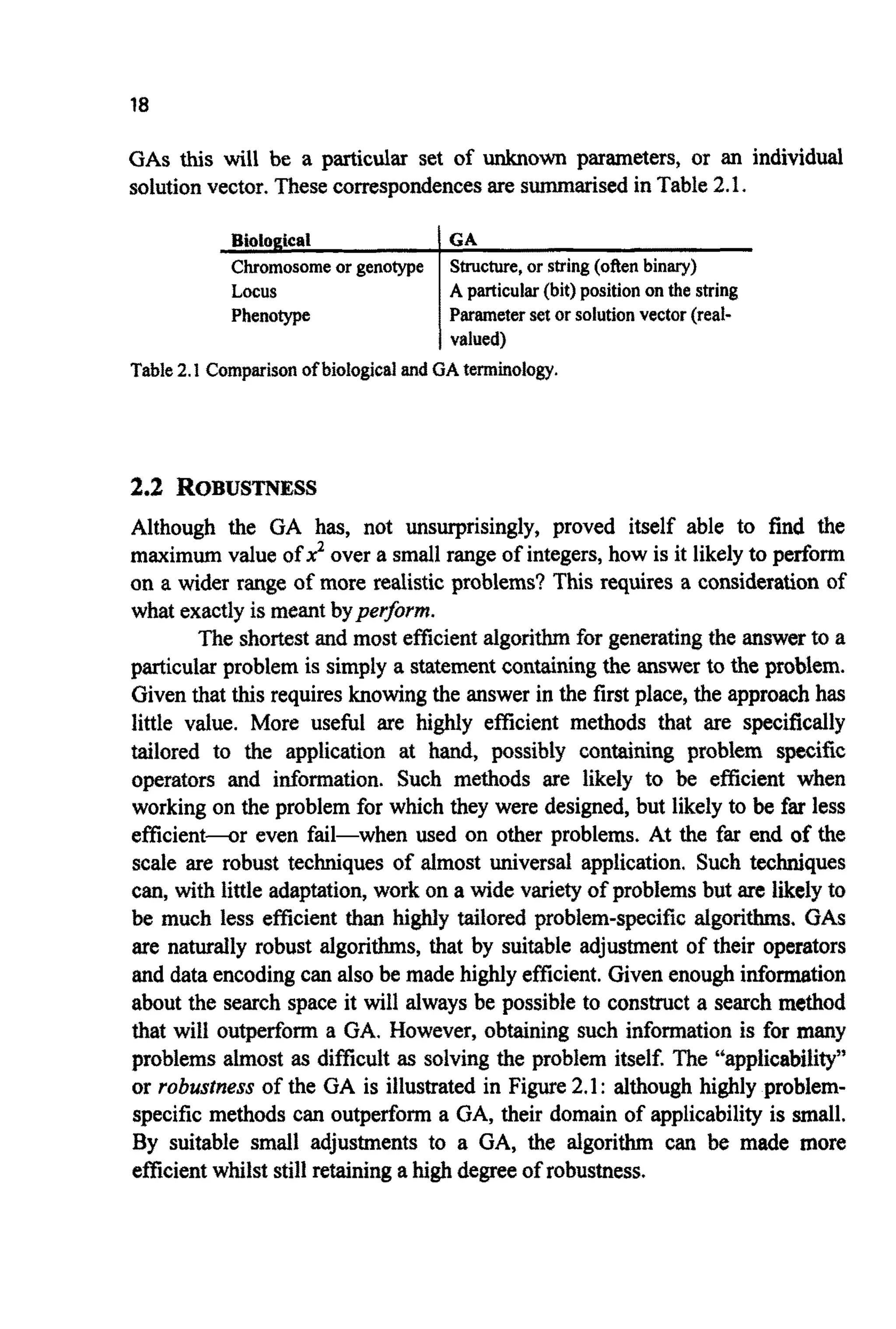
2.1 COMPARISONOF BIOLOGICALAND GA TERMINOLOGY
Much of the terminology used by the GA community is based, via analogy, on
that used by biologists. The analogies are somewhat strained, but are still
useful. The binary (or other) string can be considered to be a chromosome,and
since only individuals with a single string are considered here, this
chromosome is also the genotype. The organism, or phenotype, is then the
result produced by the expression of the genotype within the environment. In

35. 18
GAS this will be a particular set of unknown parameters, or an individual
solutionvector. Thesecorrespondencesare summarkedin Table2.1.
Locus
Phenotype
A particular(bit)positiononthe string
Parameterset orsolutionvector (real-
valued)
Table2.1Comparisonofbiological andGAterminology.
2.2 R O B U S ~ ~ S S
Although the GA has, not unsurprisingly, proved itself able to find the
maximum value of J? over a small range of integers,how is it likelyto perform
on a wider range of more realistic problems? This requires a considerationof
what exactlyis meant bype$orm.
The shortestand most efficientalgorithmfor generatingthe answerto a
particular problem is simply a statementcontainingthe answer to the problem.
Giventhat this requiresknowingthe answer in the first place, the approachhas
little value. More useful are highly efficient methods that are specifically
tailored to the application at hand, possibly c o n ~ ~ i n gproblem specific
operators and information. Such methods are likely to be efficient when
working on the problem for which they were designed, but likely to be far less
efficient-r even fail-when used on other problems. At the far end of the
scale are robust techniques of almost universal application. Such techniques
can, with little adaptation,work on a wide varietyof problemsbut are likelyto
be much less efficient than highly tailored problem-specific algorithms, GAS
are naturally robust algorithms, that by suitable adjustment of their operators
and dataencodingcan also be made highlyefficient.Givenenoughinformation
about the search space it will always be possible to construct a search method
that will o u ~ ~ o r ma GA. However, obtaining such information is for many
problems almost as difficult as solving the problem itself. The ‘4app~icability”
or robustness of the GA is illustrated in Figure2.1: although highly problem-
specific methods can outperform a GA, their domain of applicability is small.
By suitable small adjustments to a GA, the algorithm can be made more
efficientwhilst still retaininga highdegreeof robustness.

36. 19
Efficiency
A
Spectrum ofapplicable problems
Figure2.1.Comparisonof the robustnessof GA-based and more traditionalmethods.The more
robust the algorithm the greater the range of problems it can be applied to. A tailor-made
method such as a traditional calculus based algorithm might be highly efficient for some
problems,butwill fail on others. GASare naturallyrobustand therefore effectiveacross a wide
rangeofproblems.
2.3 NON-INTEGERUNKNOWNS
In Chapter 1integer-valuedparameterswere representedas binary strings.This
representation must now be adapted to allow for real-valued parameters. This
requires providing a binary representation of numbers such as 2.39~10-~or
-4.91. (Another approach discussed later is the use of a real-valued
representationwithin the GAYbut this requiresthe redefinition of several of the
GA operators.) There are many ways of doing this;however the most common
is by a linear mappingbetween the real numbersand a binary representationof
fixed length.
To carry out this transformation,the binary string(or genotype)is firstly
converted to a base-10 integer, z. This integer is then transformed to a real
number, r, using:

37. 20
The values of m and c depend on the location and width of the search space.
Expressionsfor m and c can be derived from the two simultaneousequations:
and
r,, = mz,, +c (2.3)
where rmin,rmm,zminand z,, represent the minimum and maximum possible
parameters in real and integer representationsrespectively.The smallest binary
number that can be represented is of the form 000....0 which equates to 0 in
base-10,so z,,, = 0. Zmm is given by:
z,, = 2' -1 (2.4)
where 1 is the length of the binary string used.
Subtracting(2.2) from (2.3) gives:
or
Applying (2.4) and rememberingthat Zmin = 0 gives:
Finally,rearranging(2.2) gives:
or (aszmin= 0)

38. c =r,," .
~ u ~ t i o n s(2.1),(2.5)and (2.6)then definetherequired~ansfo~ation:
(2.7)
ANEXAMPLE
Given a problem wherethe unknown parameterx being sought is known to lie
between 2.2 and 3.9, the binary string 10101is mapped to this spaceas follows:
x = 10101 thereforez = 21 .
Using (2.7):
A QUESTIONOFACCURACY
In the example above, 10101was mapped to a real number between 2.2 and 3.
The next binary number above lO1Of is 10110= 22, which, using (2.7) implies
r =3.4065. This identifiesa problem: it is not possible to specify any number
between 3.3516and 3.4065.
This is a fundamental problem with this type of representation. The
only way to improveaccuracyis eitherto reducethe size of the search space,or
to increase the length of the strings used to represent the unknowns. It is
possible to use different presentations that remove this problem [MI94];
however for most problems this proves unnecessary. By not making the search
spacelargerthan required and by choosinga suitablestringlength,the required
accuracy can usuallybe maintained. (I =20 impliesan accuracybetter than one
part in a million.) For problems with a large n ~ b e rof owns it is
important to use the smallest possible string length for each parameter. This
requirementis discussedin more detail in the Chapter6.

39. 22
COMPLEXNUMBERS
Problems with complex-valued unknowns can be tackled by treating the real
and imaginary parts as a pair of separate real parameters. Thus the number of
unknownsis doubled.
2.4 MULTIPARAMETERPROBLEMS
Extending the representationto problems with more than one unknown proves
to be particularly simple. The A4unknowns are each represented as sub-strings
of length 1, These sub-stringsare then concatenated(joined together)to form an
individualpopulation member of length L, where:
M
L=Cl,.
j-l
For example, given a problem with two unknowns a and b, then if a = 10110
and b = 11000 for one guess at the solution, then by concatenation, the
genotype is a CB b = 1011011000.
At this point two things should be made clear: firstly, there is no need
for the sub-strings used to represent a and b to be of the same length; this
allows varying degrees of accuracy to be assignedto different parameters; this,
in turn, can greatly speed the search. Secondly, it should be realised that, in
general, the crossover cut point will not be between parameters but within a
parameter. On first association with GASthis cutting of parameter strings into
parts and gluing them back together seems most unlikely to lead to much more
than a random search. Why such an approach might be effective is the subject
of Chapter 3.
2.5 MUTATION
In the natural world, several processes can cause mutation, the simplest being
an error during replication. (Rates for bacteria are approximately 2x10e3per
genome per generation [FU90, BA96,p19].) With a simple binary
representation, mutation is particularly easy to implement. With each new
generationthe whole population is swept,with everybit position in everystring
visited and very occasionallya 1 is flipped to a 0 or vice versa. The probability
of mutation, P, is typically of the order 0,001, i.e. one bit in every thousand
will be mutated. However, just like everything else about GAS, the correct
setting for P, will be problem dependent. (Many have used P,,,=: 1/L, others

40. 23
[SC89a] P,,,= l/(NdL ), where N is the population size). It is probablytrue that
too low a rate is likely to be less disastrous than too high a rate for most
problems.
Many other mutation operators have been suggested, some of which
will be considered in later chapters. Some authors [e.g. DA911 carry out
mutation by visiting each bit position, throwing at random a 0 or a 1, and
replacingthe existingbit withthis new value. As there is a 50% probabilitythat
the pre-existing bit and the replacement one are identical, mutation will only
occur at half the rate suggested by the value of P,,,.It is important to know
which method is being used when trying to duplicate and extend the work of
others.
2.6 SELECTION
Thus far,the selectionoperator has been particularly simple: the best 50% are
selected to reproduce and the rest thrown away. This is a practical method but
not the most common. One reason for this is that althoughit allows the best to
reproduce (and stops the worst); it makes no distinction between “good” and
“very good”. Also, ratherthan only allowingpoor solutionsto go forwardto the
next generation with a much lower probability, it simply annihilates them
(much reducing the genetic diversity of the population). A more common
selectionoperatorisptness-proportional,or roulette wheel, selection.With this
approach the probability of selection is proportional to an individual‘sfitness.
The analogy with a roulette wheel arises because one can imagine the whole
population forming a roulette wheel with the size of any individual’s slot
proportional to its fitness. The wheel is then spun and the figurative “ball”
thrown in. The probability of the ball coming to rest in any particular slot is
proportional to the arc of the slot and thus to the fitness of the corresponding
individual. The approach is illustrated in Figure 2.2 for a population of six
individuals (a, by c, d, e and f) of fitness 2.7, 4.5, 1.1, 3.2, 1.3 and 7.3
respectively.

41. 24
L 7.3-,..-
e, 1.3
b, 4.5
Figure 2.2. Roulette wheel selection. The greater an individual's fitness the larger its slot and
the higher its chanceof going forward to the next generation.
Implementing this operator is easier than it might seem. The
circumferenceof the wheel is given by the sum of the population's fitness and
the ball is represented by a random number between 0 and this sum. To
discover which individuai's slot the ball fell into, the fitness of the population
members are added together one at a time, but this time stopping when thisnew
sumexceeds the random number. At this point the last individual to be added is
the selectedind~vidual.The algorithmis summarised in below:
1.
2.
3.
Sum the fitness of all the population members. Call this sum&um.
Choosea random number, Rs,between 0 andfsum.
Add together the fitness of the population members (one at a time)
stopping immediatelywhen the sum is greater than R,. The last individual
added is the selected individual and a copy is passed to the next
generation.
Algorithm2. Implementingfitness-proportionalselection.
The selectionmechanism is applied twice (from Step 2) in order to select a pair
of individualsto undergo, or not to undergo, crossover. Selection is continued
until N (the population size, assumed to be even) individuals have been
selected.
In this text the type of selectionused is indicated by the value of v,, with
v, = I:indicatingfitness-proportional(roulettewheel) selection.

42. 25
2.7 ELITISM
Fitness-proportional selectiondoes not guarantee the selectionof any particular
individual, including the fittest. Unless the fittest individual is much, much
fitterthanany other it will occasionally not be selected.To not be selectedis to
die. Thus with fitness-proportionalselection the best solution to the problem
discovered so far can be regularly thrown away. Although it appears
counterproductive, this can be advantageous for some problems because it
slows the algorithm, allowing it to explore more of the search space before
convergence.This balance between the exploration of the search space and the
exploitation of discoveries made within the space is a recurrent theme in GA
theory. The more exploitation that is made the faster the progress of the
algorithm, but the greater the possibility of the algorithm failing to finally
locate the true global optimum. For many applicationsthe search speed can be
greatly improved by not losingthe best, or elite,member between generations.
Ensuring the propagation of the elite member is termed elitism and
requires that not only is the elite member selected, but a copy of it does not
become disruptedby crossoveror mutation.
In this text, the use of elitism is indicated by E (which can only take the
value 0 or 1); if E = 1 then elitism is being applied, if E = 0 then elitism is not
applied.
2.8 CROSSOVER
The Little Genetic Algorithm uses single point crossover as the recombination
operator (in the natural world, between one and eight crossover points have
been reported [GOT89,BA96,p181). The pairs of individuals selected undergo
crossover with probability P,. A random number R, is generated in the range
0-1, and the individuals undergo crossover if and only if R,IP,,otherwisethe
pair proceed without crossover. Typical values of P,are 0.4to 0.9. (If P,= 0.5
then half the new population will be formed by selection and crossover, and
half by selectionalone.)
Without crossover,the average fitness of the population,f,,, will climb
until it equals the fitness of the fittest member,f,,. After this point it can only
improve via mutation. Crossover provides a method whereby information for
differing solutions can be melded to allow the exploration of new parts of the
searchspace.
As described in Chapter 1, single point crossover proceeds by cutting
the pair of selected strings at a random locus (picked by throwing a random

43. 26
number, RL,between 1 and L - 1) and swapping the tails to create two child
strings. For example, if RL= 4, then:
Parents Children
1010/0010101
I I I I/l I I I I I I
1010/11I I I I I
1111/0010101
The new population now consists of N individuals (the same number as
the original population) created by selection and crossover. Mutation then
operates on the whole population except the elite member (if elitism is being
applied). Once this is done, the old population is replaced by the new one and
the generationalcounter,g, incrementedby one.
2.9 INITIALISATION
Although as discussed in Chapter 1 the initial population is usually chosen at
random, there are other possibilities. One possibility [BR91]is to carryout a
series of initialisationsfor each individual and then pick the highest performing
values. Alternatively, estimations can be made by other methods in an attempt
to locate approximate solutions, and the algorithm can be started from such
points.
2.10 THELITTLEGENETICALGORITHM
Having now described how multi-parameter problems with non-integer
unknowns can be tackled, and defined the mutation, selection, crossover and
elitism operators, this knowledge can be brought together within a singular
algorithm (Algorithm 3):

44. 27
I1. Generate an initial (g= 1) populationof random binary stringsof length
zlk,where M is the number of unknowns and 1, the length of binary
stringrequiredby any unknown k.In generallk f 4;kf j .
2. Decode each individual,i, within the population to integersZl,k and then
to real numbers rl,k, to obtainthe unknownparameters.
3. Test each individual in turn on the problem at hand and convert the
objective function or performance, Sat, of each individual to a fitnessf;,
where a better solutionimpliesa higher fitness.
4. Select, by using fitness proportional selection,pairs of individuals and
apply with probability P, single point crossover. Repeat until a new
temporarypopulationof N individualsis formed.
5. Apply the mutation operator to every individual in the temporary
population, by stepping bit-wise through each string, occasionally
flipping a 0 to a 1 or vice versa. The probability of any bit mutating is
given by P,,,and istypicallyvery small(for example,0.001).
6. If elitism is required, and the temporary population does not contain a
copy of an individual with at least the fitness of the elite member,
replace (at random) one member of the temporary population with the
elitemember.
7. Replacethe old populationby the new temporarygeneration.
8. Increment,by 1,the generationalcounter (i.e. g =g + 1) and repeat from
Step2 until G generationshave elapsed.
Jgorithtn3. The Little GeneticAlgorithm.
M
k-1
USINGLGA
For many applications requiring the near optimisation of real or complex
valued functions, LGA is a suitablealgorithm. However,as mentioned several
times already, the correct choice of algorithm is highlygroblemdependent and
readers are encouragedto searchthe literaturefor successfulapplicationsof the
technique to problems similar to their own. It may also prove worthwhile to
consider some of the advanced operators discussed in Chapter4. The
applicationof GASto help solve difficultproblems has a long history and the
number of adaptations to the basic technique is growing all the time. An
algorithm as simpleas LGA will not be suitablefor all problemsby any means.

45. 28
INSTALLINGAND R ~ N N ~ N ~LGADOS
The disk enclosed with this book contains an implementation (LGADOS) of
the LGA algorithm (although with 4 = fk, for allj and k,i.e. all unknowns are
represented with identica~ length strings). Both an ~ c o m p i l ~
(LGADOS.BAS) and a compiled version (LGADOS.EXE) are included. The
compiled version is designed for use with some of the exercises includedat the
end of chapters. The ~ c o m p i ~ e dversion can be adapted €or use with other
problems.
A listing (in BASIC) of the program is given both on the disk and in
AppendixB. BASIC has been used for several reasons. Firstly, it is one of the
easiest computer languages to ~ d e r s ~ dand should cause few problems for
those with experiencein FORTRAN,PASCALor C. Secondly,it complements
code written in PASCAL and C published in other introducto~text books
([GO891 and [MI941 respectively). The disk also contains translations of the
code into FORTRAN, PASCAL and C. To ensuremaximum compatibili~with
the text, these are near direct translationsfrom the BASIC code and therefore
do not represent the best way of coding a GA in these languages. Those
preferring to use a more professional FORTRAN GA should visit David
Carroll's web site (see AppendixA) and ~ u ~ l o a ~hisGA code.
Updated versions of the programs will be found at
http://www,ex.ac.uk/cee/ga/ .This site should be visited and any updates
d~wn~oadedbeforethe programsare used.
Lastly,most IBM compatiblepersonal computersusing ~ i n d o w s3.x or
DOS 6.x will have access to QBASIC-the e n v i r o ~ e n ~used to write LGA-
thereby allowing a~te~tionsto be made easily and the student exercises
completed. However, QBASIC does not contain a compiler, and therefore
LGADOS will run rather slowly on anything but the simplest problem. If you
wish to adapt the code to use on your own problems you will probably need
either to purchase a BASICcompiler (sharewareones EW: available), use one of
the translationson the disk (LGADOS.F, LGADOS.PAS and LOAD0S.C) or
convert the code to a language for which you already have a compiler. This
conversionshould be relativelyeasy as no overlyspecial structuresor operators
have been used.
A word of caution: LGADUS has been written with simplicity rather
than efficiency in mind and as such does not represent good p r o ~ i n g
practice. There are much faster ways of performingsome of the operationsand
better languages than BASIC in which to write such code. Those without the
required knowledge may well find it advisable to enlist the help of a more
experienced programmer to produce more efficient code. Having said this, in

46. 29
the majority of real-world problems to which GASare applied, the time taken
for the GA to cycle through a generation of selection,crossoverand mutation is
much less than the time taken to estimate the objective functions, and hence,
the fitness of the individuals. This is a very different situation to that
encountered when examining the performance of a GA on established test
problems. The functionestimationsin such tests are typically much simplerand
much quicker to calculatethan their real-world counterparts-which might take
several minutes per estimation. This implies that, in the majority of cases, time
is better spent producing code that can carry out these function evaluations as
rapidly as possible, rather than considering how to increase the speed of the
GA’s operators.BASIC allows-as do many other languages-the inclusionof
mixed language routines. This means it is easy to add pre-existing routines to
carry out the functionevaluations.
Another sensible approach to developingapplicationsis to use some of
the GA code available on the World Wide Web (see Appendix A), or contact a
researcher who has recently published in a closely related field using GASand
enthusethem into helping out.
LGADOS itself is examined in detail in Chapter 5, a quick glance at
which shows that the program is quite short, and capable readers are strongly
encouraged to write their own version, in the language of their choice. This is
recommended even for those that may end up using someone else’s code to
solve research problems, as it ensures a full understanding of the processes
involved.
To run the compiled version, copy LGADOS.EXE to a new sub-
directory (folder) on your hard drive and type LGADOS from that directory if
using DOS, or double-click on LGADOS.EXE from File Manager (or
Explorer).
The user is presented with a series of options for N, P,, P m etc. and
possibletest problems (Figure 2.3).
Output is via two files: LGADOS.RES and LGADOS.ALL.
LGADOS.RES lists the generation, g;fitness,fmm,of the highest performing
individual; the average fitness of the generation, fme;and the unknown
parameter values, Q,contained in the fittest individual. LGADOS.ALL lists g,
f, rk and the binary chromosome C for all individuals in all generations, and
hence can be very large. The files are comma separatedand can be loaded into
most spreadsheetsfor analysis and data plotting.

47. 30
N, Population S i z e (muat be oven) = 20
1, Subetring Longth (all sub-atrings have the 8.m. length) = 10
G, Wax. Generation .I 50
Pc, Crorrover Probability (2-0 and <-l) = 0.65
Pnr, Mutation Probability ( 2 4 and cl) = 0.001
e, Blitiam (1-on, O=off) - 0
am, Scaling Conatant (a value of 0 implies no scaling) m 0
Problem (l-Fl, 2mF2, 3-83, 4rF4, 5-f^2) - 2
Figure 2.3. A completed input screen for LGADOSEXE. The meaning of cm will described
later,but it shouldbe setto zero for now.
Totest LGADOS,and the stochasticnatureof GAS,asimpleexample:
can now be completedusing LGADOS. The followingsettingsshouldbe used:
N=20
l = 10
G=20
P,= 0.6
Pm= 0.01
& = O
c, =0
Problem=fz
After setting these, press ENTER. LGADOS will display a simple
listing of the average and best fitness within a single generation, together with
the best estimate of x. These results are also stored within the file
LGAD0S.RES.
When LGA has runthroughall 20 generationsprint out LGADOSXES,
run the program again, and print LGADOSRES. Finally repeat this process
oncemore. If you comparethe three setsof results they shouldbe substantially
different. (If not, you were simply fortunate.) The reasons for these differences
are the stochastic processes embedded within the algorithm, i.e. the use of
random numbers to pick individuals to mate, crossover sites and mutation
locations. Therefore no two runs of a GA are ever likely to produce the same
series of results (unless the random number generator was seeded with the
same number both times). This is important to remember. If computer
experiments are being run in an attempt to ascertain the best values of the
internalGA settings(Pm,Pc etc.) for a particular problem, the results from one

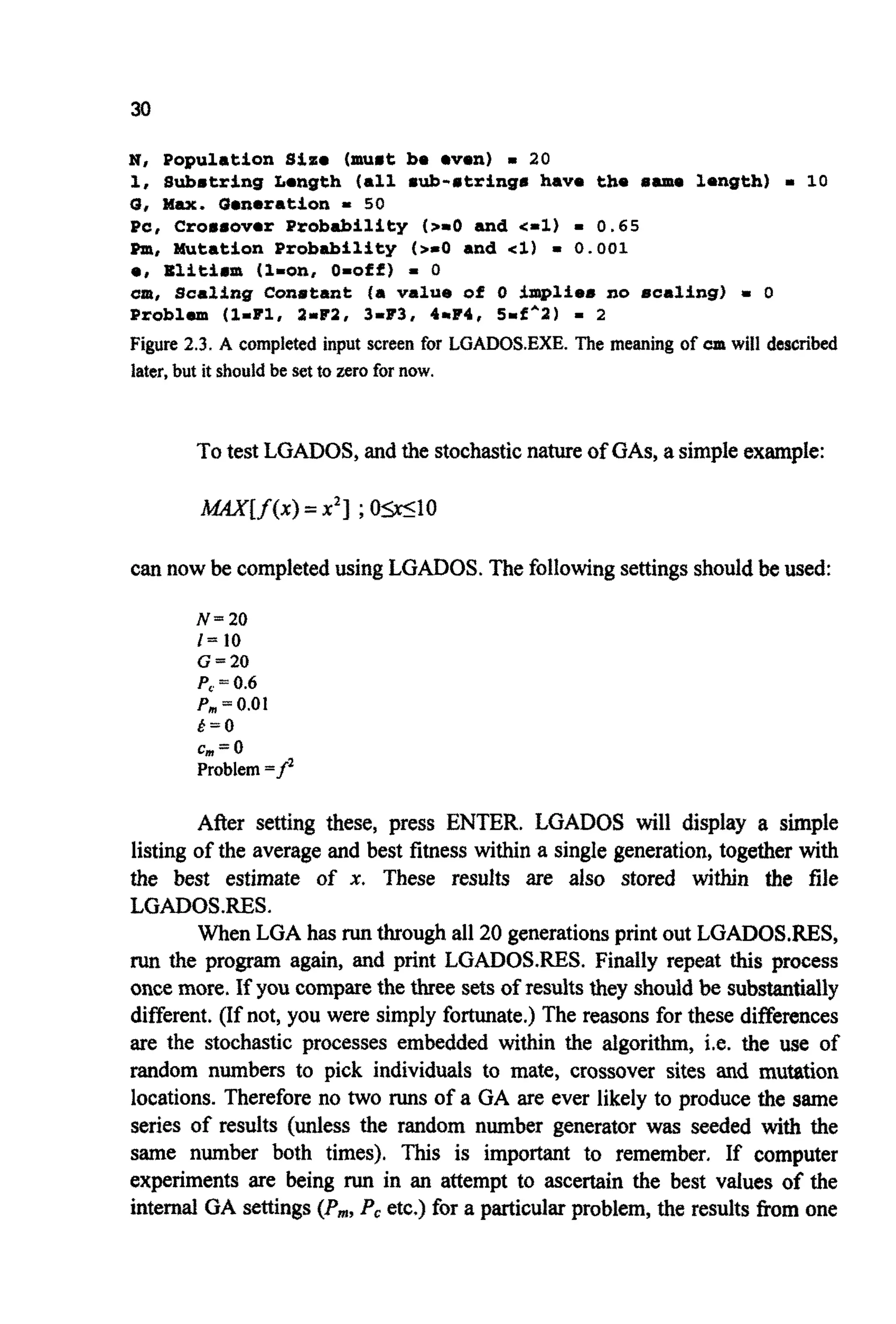
48. 31
GA run shouldnot be relied upon to be meaningfuI.Rapid, or slow, progressof
the GA could well be simply the result of the particular random numbers
encountered(Figure2.4).
Figure 2.4.Sample resultsfiom multipleruns of LGADOSonthe problem MAX[Ax) =xz] ;0
Sx <lo.TheMLS show very differentcharacteristicsVw plotted).
It should be noted that although averaging solution vectors (i.e.
parametervalues) produced by GASprovides a way of monitoringprogress and
producing pedomance measures for the algorithm, there is little point in
averaging sofution vectors when dealing with real problems once the i n t e d
GA settings have been established. In fact, not only is averaging solution
vectors of little benefit, but it can also lead to quite erroneoussolutions. Figure
2.5 shows a hypothetical one-dimensional fitness landscape. If two runs of a
GA produce the solutions GI and a2 respectively, then the mean of these
solutionsis ~ 3 - a very poor result. Sucha spacewould be bettertackled with a
long GA run,whilst ensuring the population remained diverse, or by multiple
runsdisregardingall but the best solution.
In this text, the number of multiple runs made to produce a result is
denoted by X.

49. 32
8 -
6 -
' I .
4 -
2 -
Figure 2.5. A potential pitfall of averaging solution vectors from multiple runs of a GA,
U] = (a1 .t u$2.
2.11 OTHER E V O ~ U T I O N ~ Y~ P R O A C ~ E S
Genetic algorithms are not the only evolutionary approach to search and
optimisation.
Evolutionary Programming [F066] typically uses a representation
tailored to the problem (e.g. reals, not binary). All N individualsare selected
and a representation specific, adaptive mutation operator used to produce N
offspring. The next generation is then selected from the 2N individualsvia a
fitness-biasedselectionoperator.
Evolution Strategies originally used N = I togetherwith a mutation and
selection operator. This has been extended [SC81J to N 1 1, with mutation and
recombinaiionto create more than N offspring. Selectionis then used to return
the populationto N individuals.
For an overview of such approaches see [BA96, p57-60, BA91 and
SP931.

50. 33
2.12 SUMMARY
In this chapter the algorithmhas been extended to deal with multi-dimensional
problems of non-integer unknowns. The selection operator has also been
improved to allow use to be made of the distinction between “good” and “very
good”.
A comparisonof biological and GA terminology has been made and the
robustnessof the algorithmqualitativelycompared to more traditional methods.
The problem of limited accuracy caused by discretisation of the search
space, implied by the use of a fixed binary representation, has been considered
and seen to cause few difficultiesfor many problems.
A simple genetic algorithm, LGA, has been introduced and used to
solve a trivial problem. This has allowed one of the potential pitfalls caused by
the stochasticnature of the method to be discussed.
In the next chapter, some of the reasons why GAS work well across a
wide range of problemswill be furtherconsidered.
2.13 EXERCISES
1.
2.
3.
4.
5.
6.
Within the terminology used in GAS, characterise the difference between
the genotypeand the phenotype.
Derive (2.7)
Given I = 4, what is the highest fitness that can be found by a binary
encoded GA for the problem MAX[sin’’(x)]; 0 Ix I3?
If N = 6 withfi = 1,fi = 2,f3= 3,f4= 4,h= 5 andfa = 6, how many times
is the individual with f=4 likely to be picked by fitness proportional
selection in a single generation? What is the minimum and maximum
possible number of times the individual withf= 6 might be picked? What
problem does this indicate could arise in a GA using fitness proportional
selection?
Write, in a programming language of your choice, a GA similarto LGA.
Use LGADOS, or your own code, to study the evolution of a population
whilst it explores the search space given by f = x s i n 4( x i ) ;0 5X i IA ,
2
1-1

51. 34
i = 1,2 .Plot the movements of the population acrossthe searchspace (as a
hction ofg)as aseries of (XI, x2,f) surface plots.

52. 35
CHAPTER3
Although the roots of evolutionary inspired computing can be traced back to
the earliest days of computer science, genetic algorithms themselves were
invented in the 1960's by John Holland. His reasons for studying such systems
went beyond a desire for a better search and opti~sationalgorithm. Such
methods were (and stilf are) considered helpfirf abstractions for studying
evolution itself in both natural and artificial settings. His book Adapiafionin
Natsrral and Ari@cialsystems from 1975 (and now updated) was, and still is,
inspirational.
With the aid of his students Holland developed the GA m e r during
the 1970'9, He also produced a theoretical framework for ~ d e r s ~ d i n ghow
GAS actually work. Until relatively recently this schema theory formed the
basis of most theoretical work on the topic.
Exactlywhy GeneticAlgorithmswork is a subject of somecontroversy,
with much more work being required before all questions are finallyanswered.
However the subject is not without foundations. These fo~dationshave
emerged from two separatedirections. One is based on attempts to provide a
mathematical analysis of the underlying processes, the other on computer
simulationson hctions that reflect aspectsof some of the problems to which
GAShave been applied(or onesthat GASmight havedifficultywith),
Thereare somevery good reasonswhy, even asp~ctjtionersratherthan
theorists, it might be beneficial for the subjectto have a theoreticalfo~dation.
In particular, a knowledgeof the type of problems where GASmight, or might
not, perform well (or even work) would be extremely useful. Equally useful
would be guidance on the degree to which such algorithms might outperform
moretraditionalmethods.
Much of the work in this area is not suitable for an i n ~ o d u c t o ~text"
For an overview the reader should see the series Fo~ndu~io~sof Genetic
A Z g ~ ~ ~ f ~ ~ sm91,WH93,WH95]. However, a brief consideration of the
subjectiswe1worththe modestef€ortrequired.Inthe following,both a largely

53. 36
theoretical method and a more applied approach will be considered. The
theoretical work is based on Holland’soriginal schematheorem, popularisedby
Goldberg [G089]. The applied work is based on the systematic adjustment of
internal settingswhen using a GA to tackle a seriesof test functions.
Both approaches are required because while most theoretical work on
GAShas concentrated on binary alphabets (i.e. strings containing only 0’sand
l’s), fitness-proportional selection and pseudoboolean functions (i.e. functions
expressed using 0’s and l’s), practitioners have used a vast array of
representations and selection methods. Results therefore do not necessarily
translate between these approaches, implyingyet more caution when choosing
settingsand decidingbetween various algorithmsetc.
3.1 HISTOIUCALTEST F”CTI0NS
Before looking at schema theory there is a need to look at some of the
theoretical test functions (or artficial landscapes) used to examine the
performanceof varying GAS.These functions are not only of historical interest.
They, together with more complex functions, are often suited to the testing of
user developedcodes.
Although typical test functions are very useful because they allow for
easy comparisons with other methods, they may have little relevance to real-
world problems. Thus care must be taken not to jump to conclusions about
what is best in the way of algorithmor settings.Often such functionshave been
too simple, too regular and of too low a dimensionto represent real problems
(see comments in [DABlb] and EWH95al). Bgck [BA96,p138] suggests sets of
functions should be used, with the group covering several important features.
The set should:
1. consist exclusively of functions that are scalable with respect to their
dimension M, i.e. the number of unknowns in the problem can be changed
at will;
2. includea unimodalfie. singlepeaked), continuo^ function for c o m p ~ ~ n
of convergencevelocity(see below);
3. include a step function with several flat plateaux of different heights in
order to test the behaviour of the algorithm in case of the absence of any
local gradient information;and

54. 37
4. cover multimodal(i.e. multi-peaked) functionsof differingcomplexity.
Although many others had been investigating genetic algorithms for
some time, De Jong's dissertation (published in 1975) Analysis of the
Behavlour of a Class of Genetic Adaptive Systems [DE75] has proven to be a
milestone. One reason for this is the way he carried out his computer
experiments, carefully adjusting a single GA setting or operator at a time. The
other is the range of functions(or problems)on which he chose to test the GA.
These functions, together with additions, are still used today by some to make
initial estimates of the performance of their own GAS.In fact it is well worth
coding up a subset of these functions if you are writing your own GA (for
function optimisation), simply so that you can check that all is proceeding
accordingto plan within your program. If you are using a GA you did not write
then this is still a worthwhile exercise to prove that you have understood the
instructions. The idea of using test functions to probe the mechanics and
performance of evolutionary algorithms has continued to the present day. For
an excellentmodem examplesee Back's recent book [BA96].
De Jong's suit of functions ranged from simple unimodal functions of
few dimensions to highly multimodal functions in many dimensions. Unlike
most research problems, all of them are very quickly calculated by computer
and therefore many generations and experiments can be run in a short time.
Adapted versions of three of the functions (together with some additions) are
listed in Table 3.1, and two-dimensionalversions of several of them presented
in Figures 3.la to 3.ld.
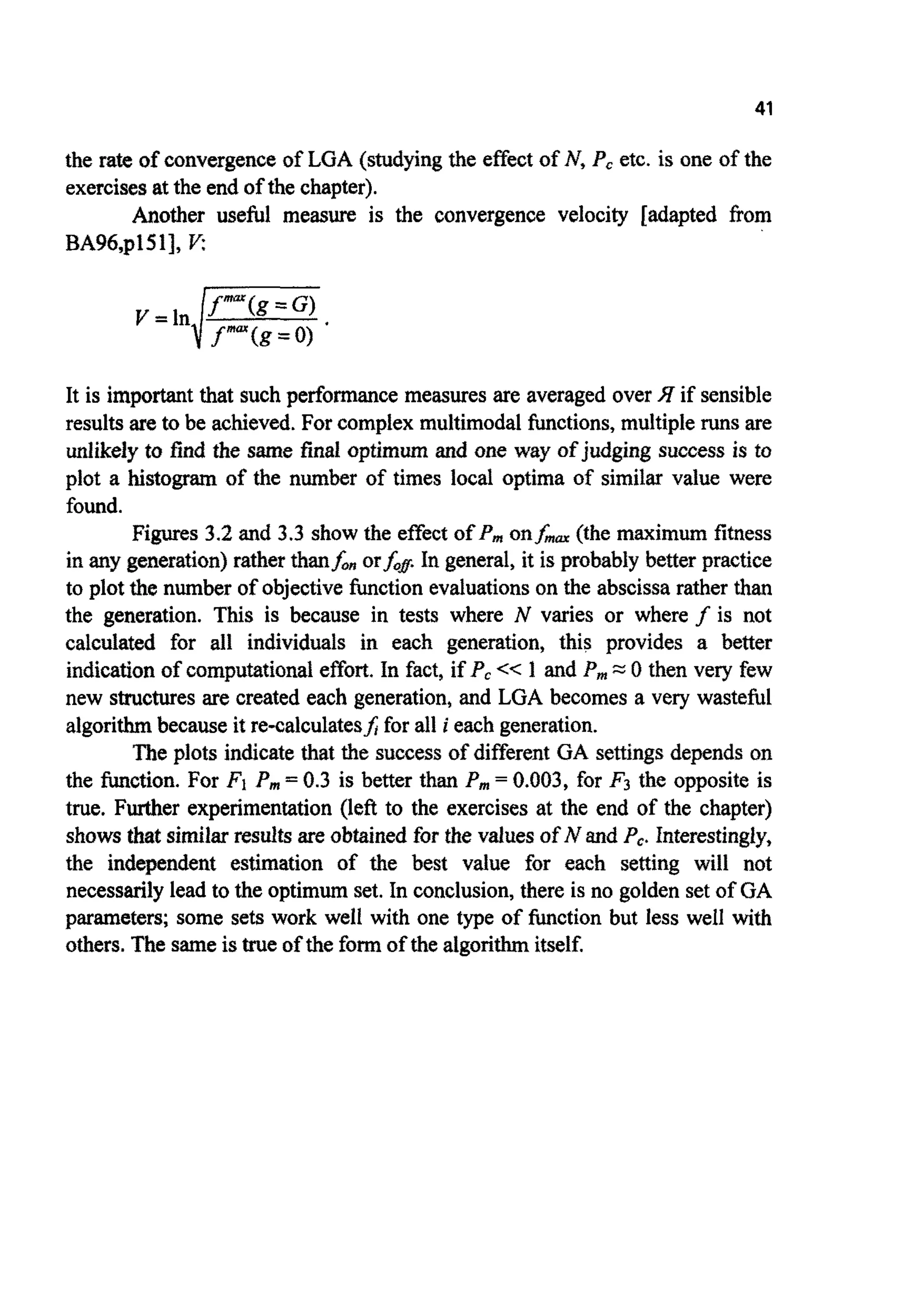
MEASURINGPERFORMANCE
De Jong used two measures of the progress of the algorithm: the off-line
performance and the on-line performance. The off-line performancej& is a
runningaverageof the fitnessof the best individual,f-, in the population:
The on-line performance,f, is the average of all fitness valuesJ calculated so
far. It thus includesboth good and bad guesses:

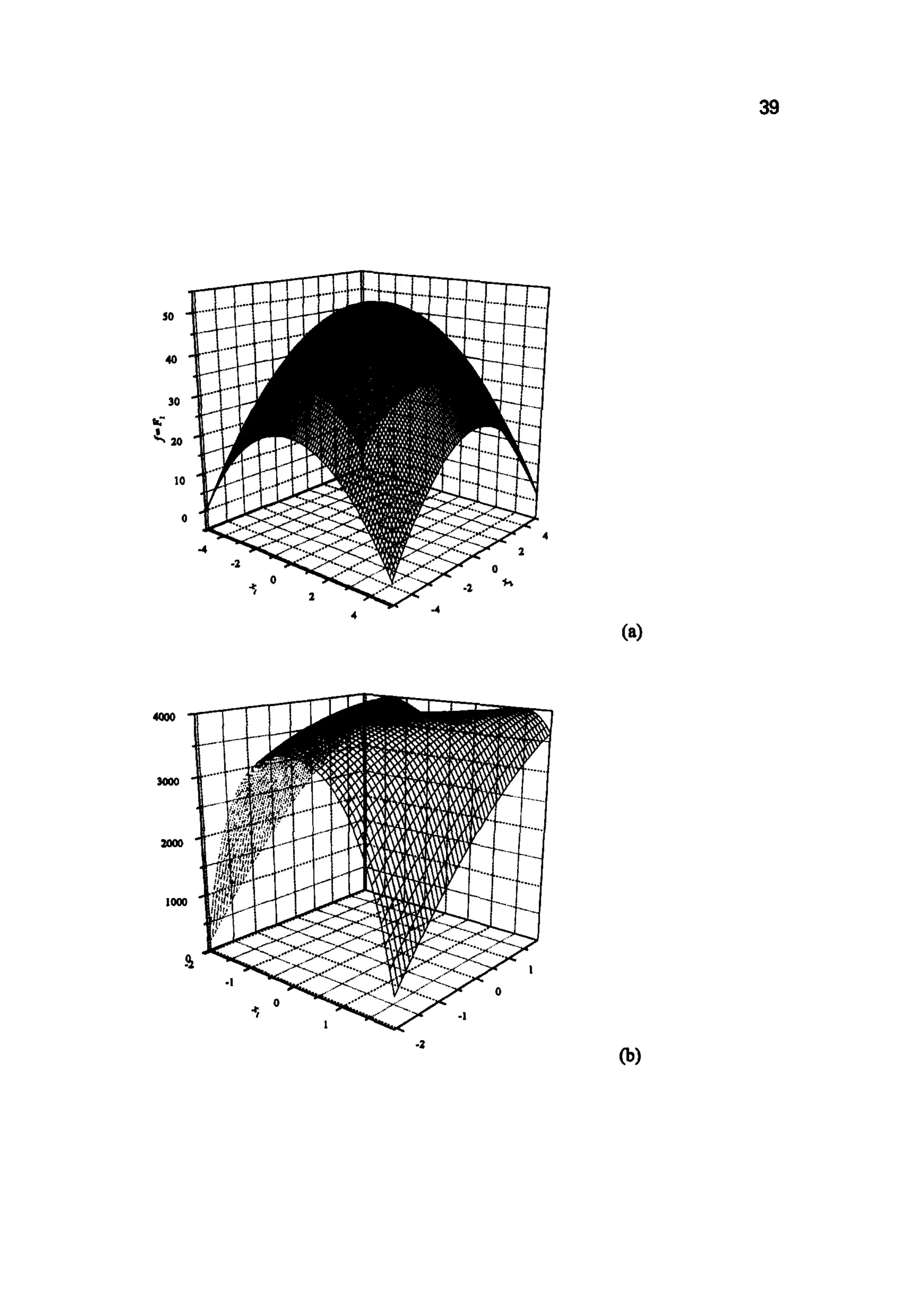
55. 38
Function
3
f= 4 = 7 9 - c x ;
1-1
f=F, =4000-100(x~-x2~+(l-xl)'
5
f = & = 26-CZNT(xJ)
]=I
( s i n , / m ) l -0.5
f=F4 ~ 0 . 5 -
(1 +0.001(x: +x;y
f = F6= A - 2 0 e x p [-0.2 p3]-
--[;m$0s(2-,i]530) +20
Limits
-5.12I~jI5.12
-2.048 5xj 5 2.048
-5.12<xj5 5.12
-100 I X j 5 100
-20Lxjs30
Table 3.1. Adapted versions of various test functions: De Jong's (Fl to F3), Davis (F4)
[DA91,SC89a] and Back (F5and F6) [BA96]. The function INT(-)returns the nearest integer
less than or equal to (-). A is chosen to ensure a maximisation problem. Back [BA96]also
presents an interesting fractal function based on the Weierstrass-Mandelbrot function
[MA83,FE88].

56. 39
2

57. 40
J , . , , , . , . ,
-100 -so 0 50 100
*I
(dl
Figures 3.1 (a) to (d). Two dimensional versions of the test functions of Table 3.1: selected
&om [DE75 and G0891, F1 to F,; and a section through the global optimum of (F4)
[DA91,SC89a].
De Jong actually used six algorithmsor reproductiveplans for his GA
experiments. Here, tests are restrictedto testing the effect of mutation rate on

58. 41
the rate of convergenceof LGA (studyingthe effect of I?, P, etc. is one of the
exercisesat the end of the chapter).
Another useful measure is the convergence velocity [adapted from
BA96q1511, Y:
It is important that such performancemeasures are averaged over if sensible
resultsare to be achieved.For complex multimodalfunctions,multiple runs are
~ ~ k e ~ yto find the same finai o p t i m ~and one way of judging success is to
plot a histogram of the number of times local optima of similar value were
found.
Figures 3.2 and 3.3 show the effect of P, onfma (the maximum fitness
in any generation)rather than&,, or&@In general, it is probably better practice
to plot the number of objective function evaluationson the abscissarather than
the generation. This is because in tests where I? varies or where f is not
calculated for all individuals in each generation, this provides a better
indication of computationaleffort. In fact, if P,<< 1 and P, =0 then very few
new structuresare created each generation, and LGA becomes a very wasteful
algorithmbecause it re-calculatesf;for all i each generation.
The plots indicate that the success of different GA settingsdepends on
the function. For F1 P m = 0.3 is better than P m = 0.003, for F3 the opposite is
true. Further experimentation (left to the exercises at the end of the chapter)
showsthat similarresuitsare obtained for the values of N and Pc. Interestingly,
the independent estimation of the best value for each setting will not
necessarilylead to the optimum set. In conclusion,there is no golden set of GA
parameters; some sets work well with one type of function but less well with
others. The sameistrue of the form of the algorithmitself.

59. 42
............................
. .,.
. . . . . . . . . . . . . .
P, =0.03
Pm=0.003.......
J- .'
7 3 1 ' ' ' ' ' ' ' ' ' '
0 3 10 I5 20 25 3
Figure 3.2. The progress of fm for test function Fl and various settings of P, (N=20,
P,=0.65,1= 10,k- l,X=20).
25
24
23
I 22
21
20
I Q
Pm=0.03
P,,=0.003
0 5 10 I5 20 25 30
g
Figure 3.3. The progress off- for test function F3 and various settings of P,,,(N=20,
P,=0.651= 10, E = 1, B= 20).

60. 43
THEPROBLEM OF CONVERGENCE
The above experiments indicate that, although LGA was able to find
approximate optimum values of the test functions quickly, its progress was by
no means linear. Initial progress is rapid and the value off- soars. However
this progressis not maintained.One clue to the reason for this behaviourcan be
gleaned if the level of geneticdiversity within the population is plotted against
generation;another from a considerationof the likelihood of progressionto the
next generationunder roulettewheel selection.
THEAPPLICATION OF SCALING
If early during a run one particularly fit individual is produced, fitness
proportional selection can allow a large number of copies to rapidly flood the
subsequent generations. Although this will give rapid convergence, the
convergence could quite possibly be erroneous or only to a local optimum.
Furthermore, during the later stages of the simulation, when many of the
individuals will be similar, fitness proportional selection will pick
approximatelyequal numbersof individuals from the range of fitnesses present
in the population. Thus there will be little pressure distinguishing between the
good and the very good.
What is needed is a method whereby particularly good individualscan
be stopped fiom running away with the population in the earlier stages, yet a
degree of selection pressure maintained in the final stages. This can be
achievedby various mechanisms;one being the use of linearfitnessscaling.
Linear fitness scaling works by pivoting the fitness of the population
members about the average population fitness. This allows an approximately
constant proportion of copies of the best individuals to be selected compared
with average individuals.Typical values for this constant, cm,are in the range
1.0 to 2.0. When cmequals 2, then approximately twice the number of best
individualswill go forwardto the next generationthan will average individuals.
To achieve this, the fitness of every population member will have to undergo a
scalingjust before selection. This scaling needs to be dynamic. The fitnesses
will need to be drawn closer togetherduringthe initialstagesand pulled further
apart during the later generations. The required scaling is achieved using the
lineartransformation:
wherefiis the true fitnessof an individual, i, andA thescaled fitness.

61. 44
As already stated, the mean fitness of the populationfoye is assumed to
remainunchanged,so:
An add~tionalrequirementisthat
Where fiatis the scaled fitnessof the best individual.
This impliesthat:
Unfortunately, such a transformation can produce negative scaled fitnesses.
These can be eliminated in various ways, the simplest (but rather crude) way
being just setting any that occur to zero. In LGADOS, setting c,,, itself to zero
stopsscalingfrom being applied.
Many other scaling procedures are possible and are discussed in the
literature. An alternativeapproachis to use a different selection mechanism,as
considered in Chapter4.
Scaling can be important with even simple problems, as the following
illustrates. LGA can be used to find the value of x which maximises
F= 1000+sin(@, 0 5x In;but as Figure 3.4 shows, there will be very little
selection pressure on individuals as they will all have near identical
performance.This impliesthat the algorithmwill proceed rather slowly.Fitness
scaling, as described above,could be used to increasethe selectionprobabilities
of better individuals. However, a simpler approachwould be via a simplenon-
dynamicdirect fitnessfunction adaptationto ensurefspans a sensiblerange i.e.
f=F - 1000. An alternative approach would be to use one of the selection
mechanismsdiscussed in the next chapter.

62. 45
0.8 -
I ' l - I . 1 . , . I 0
0.0 0.5 I .O 1.5 2.0 2.5 3.0
X
Figure 3.4. Increasing the difference between populationmembers via a simple non-dynamic
direct fitnessfunctionadaptation;F = dashed line,F - 1000= solid line.
GENETICDRIFT
The amount of diversity can be measured in several ways. An easily calculable
measure is qmm,the genotypic similarity between the string representing the
fittestindividual and all the other members of the population.
To calculate qmnxthe value of each bit in the fittest string is compared
with the value of the samebit in all the other stringsin turn. Any matchingbits
increment qmaxby 1. When all the positions have been compared the result is
normalised by dividingby the total number of bits in the other strings, i.e. the
product (N-1)L.
For example,given a population of four chromosomesof length five:
C] I O I l O
c2 O I l l l
c3 loll0
c4 l l l l 0
with CIhavingthe highest fitness,then q- is given by

63. 46
0.9
0.8
10.7
c.
0.6
0.5
2+1+3+3+2 11
(4-1)x5 15
=-=0.73 .
- _, - _ I
-
,'
-
-
-
-
Plotting il- for one of the earlier experiments gives Figure 3.5; here
the population is seen to rapidly lose its diversity if scaling is not used. By
including linear fitness scaling the diversity is seen to fall less rapidly in the
first few generations, implying a greater degree of exploration. In later
generations, qmarcontinues to rise in an almost linear fashion because of the
higher selectionpressurepresent (implying a greater degree of exploitation).
0 10 20 30 40 50
g
Figure 3.5. The progress of the similarity measure )~mnr.The use of scaling produces a more
linear growth in )lam (f=x', 0 I x In,N = 20, P,= 0.65, P, = 0.001, 1= 10, E = 0, c,,, = 0 and
1.2,J7 = 20).
3.2 SCHEMATHEORY
This is an approach introduced by Holland [H075] and popularised by
Goldberg [G089].
A schema (plural schemata) is a fixed template describing a subset of
strings with similarities at certain defined positions. Thus, strings which
contain the same schema contain, to some degree, similar information. In
keeping with the rest of this book, only binary alphabets will be considered,
allowing templates to be represented by the ternary alphabet {O,l,#}. Within

64. 45
0.8 -
I ' l - I . 1 . , . I 0
0.0 0.5 I .O 1.5 2.0 2.5 3.0
X
Figure 3.4. Increasing the difference between populationmembers via a simple non-dynamic
direct fitnessfunctionadaptation;F = dashed line,F - 1000= solid line.
GENETICDRIFT
The amount of diversity can be measured in several ways. An easily calculable
measure is qmm,the genotypic similarity between the string representing the
fittestindividual and all the other members of the population.
To calculate qmnxthe value of each bit in the fittest string is compared
with the value of the samebit in all the other stringsin turn. Any matchingbits
increment qmaxby 1. When all the positions have been compared the result is
normalised by dividingby the total number of bits in the other strings, i.e. the
product (N-1)L.
For example,given a population of four chromosomesof length five:
C] I O I l O
c2 O I l l l
c3 loll0
c4 l l l l 0
with CIhavingthe highest fitness,then q- is given by
47
any stringthe presence of the meta-symbol # at a position impliesthat either a
0 ora I could be present at that position. So for example,
I01001
Ill001
and
arebothinstancesof the schema
I##OOI.
Conversely,two examplesof schematathat are containedwithin
01011I
OI#Ill
#I01##*
are
and
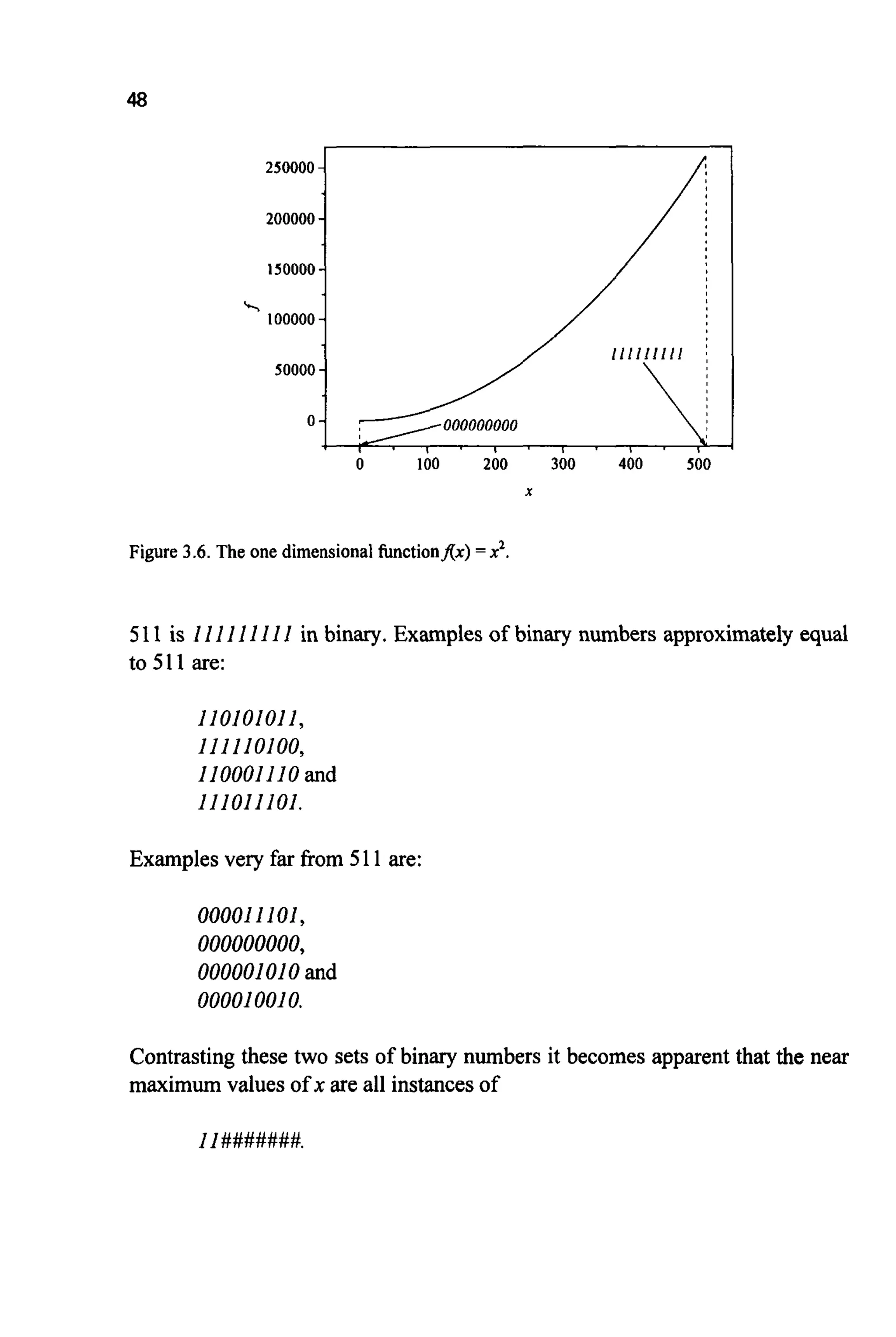
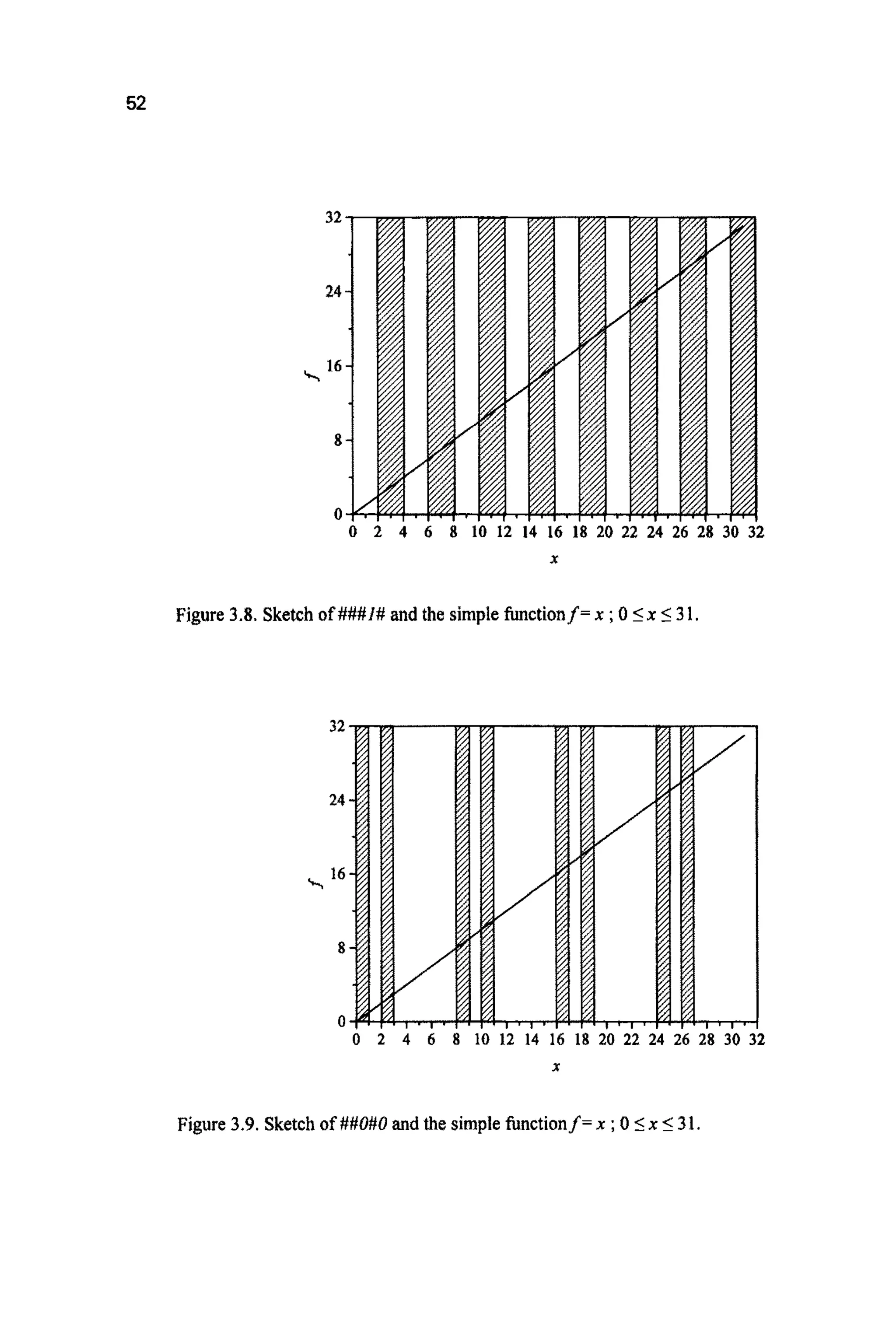
Schemata are a useful conceptual tool for severalreasons, one being that they
are simpIy a n o t a ~ o n ~~ n v e ~ e n c e .Imagine a simple o n ~ d i m e n s ~ o ~ l
problem:
MAxlf(x) =x q ;o9x 5 511
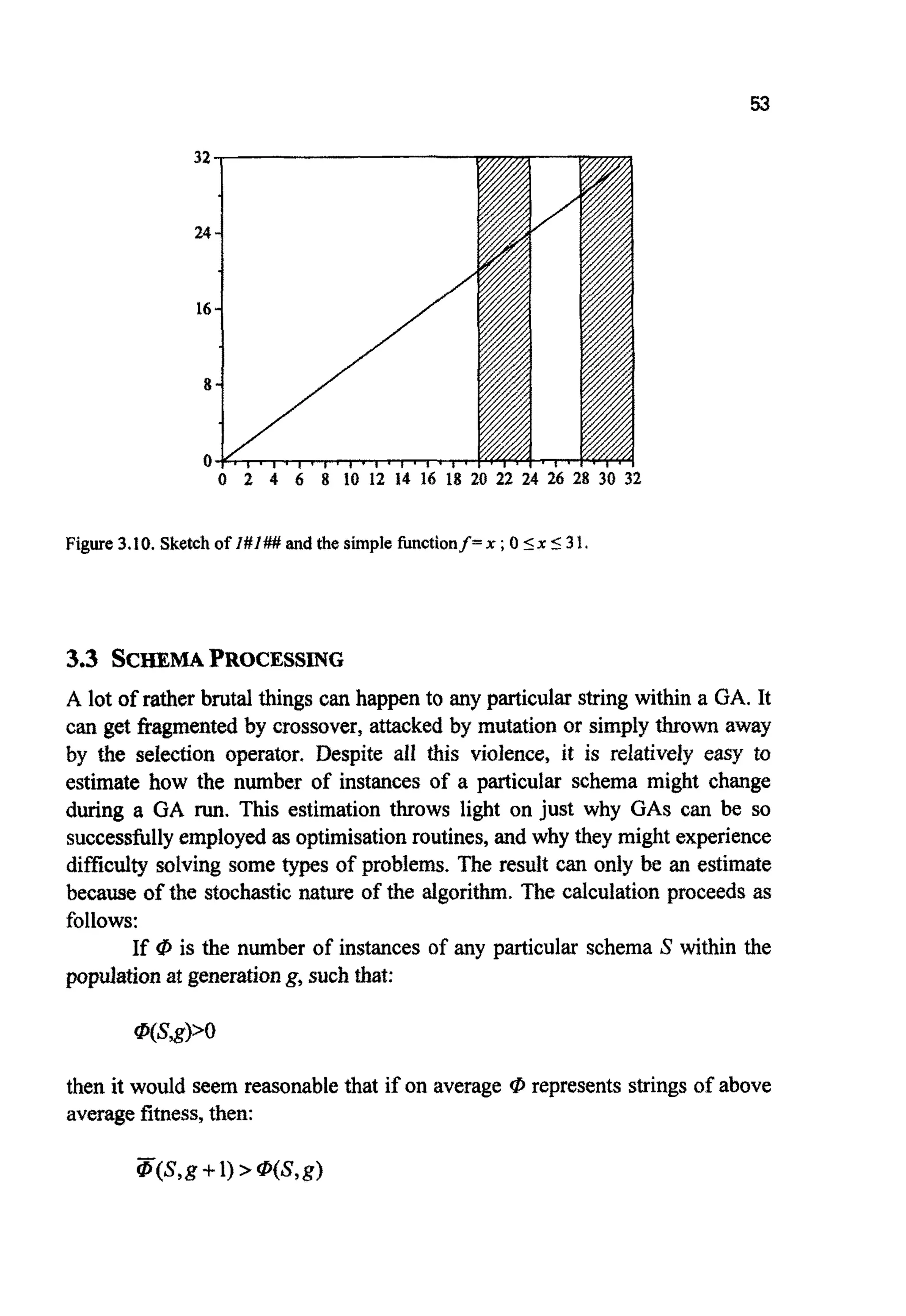
Clearly f(x) is at a maximum when x is maximum i.e. when x = 511
(Figure3.6).

65. 250000-
200000-
I50000-
'?
100000-
50000-
I * , . I . , I
0 100 200 300 400 500
X
Figure 3.6. The one dimensionalhctionflx) =xz.
511 is 11111111I in binary. Examples of binary numbers approximately equal
to 511 are:
I1010101I,
III1I0100,
110001110and
II1011101.
Examplesvery far from 51 1 are:
000011101,
000000000,
000001010 and
000010010.
Contrasting these two sets of binary numbers it becomes apparent that the near
maximum values ofx are all instancesof
II#######.

66. 49
150000-
'?
100000-
50000-
0-
Thus II####### provides a convenient notation for the numerous binary
stringsthat represent a near optimal solutionto the problem (Figure 3.7).
:/I10000000 or 384
i
250000
200000 I I#######
4 , , , . , . , . d0 100 200 300 400 500
X
Figure 3.7.Ax)=x2. The line x = 384 = IlOOOOOOO, indicates the minimum value any string
containing the schema II####### can have and is therefore the boundary of the schema. Ail
other instancesof this schemalie tothe right of this line.
There are a great number of possible schemata within a single string.
Giventhe randomly generated fourbit string,
1011
the list of allpossible schemata is
101#,
IO#I,
I#ll,
#011,
I O##,
H I # ,
1##1,
#01#,
#O#I,
##II,

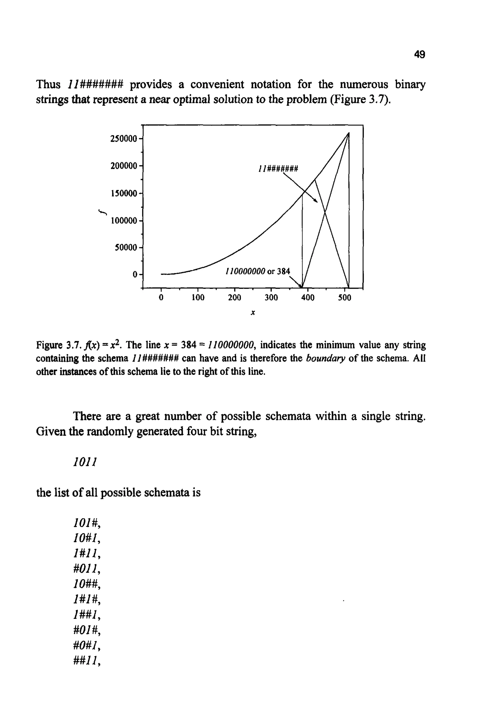
67. 1###,
#O##,
##i#,
###I,
#### and
1011,
or 16 entries. 16 = 24; for any real string of length L there are 2L possible
schemata. For an a r b i ~ ~string, each bit can take the value f or 0 or #. So
there are 3 possibilities for each bit, or 3 x 3 ~ 3 ~ 3possibilities for a string of
length4. For a stringof length 200 (a number typical of that found in many real
GA applications)there are therefore 3200 (~3x1095)schematato be found (c.f.
1080, the numberof stableparticles in the universe).
In general, for an alphabet of cardinality(or distinct characters) k,there
are (k+ 1)L schemata.For a population of N real strings there are N k ~possible
schemata. The actual number of schemata within a population is likely to be
much less than this for two reasons. Firstly, some schematacan simultaneously
represent differing strings, for example, given N = 2, L = 3 and the population
(101, I l l ) , a tableof possible schematacan easilybe formed(Table3.2).
c,= 101
#01
I # ]
10#
##I
#O#
I ##
###
101
Table3.2. Possibleschematafor a particularpopulationof 2 stringsand L = 3.
This table contains 16 schemata (8 for each string), but only 8 are unique. For
other populations this reduction may be less dramatic.If, once more, N = 2 and
I = 3, a possible population is {111,000);then there will be only one shared
schema,namely ### and hence there are 15 unique schemata. Secondly,not all
the population members themselves are likely to be unique, particularly in an
algorithm that has cycled through many generations and is near convergence.
Thus the number of schemata in the population will change as the generations
go by, but will alwaysbe <NkL.

68. 51
Not all schemata are equal. The area of the search space represented by
a schemaand the locationof this area depend on the number and location of the
meta-symbols within the schema. Schema such as I#### and O#### include
much larger regions of the search space than loll# or 0010#. Schemata are
typically classified by their de$ning length and their order. The order o of a
schemaS is the number of positions within the schema not defined by a meta-
symbol, i.e.
o ( S ) = L - m ,
where m is the number of meta-symbols present within a string of length 1. The
order is thereforeequal to the number of fixed positions within the schema:
S=#l#O#;o(S)=2
s=11001;o(s) = 5
s= #####; o(S)= 0
S= llOI#; o(S) = 4
The defining length d specifies the distance between the first and last
non meta-symbol characters within the string:
S= #1#0#;d(S)= 4- 2 = 2
S= 1101#;d(S)= 4- 1= 3
S= 11001;d(S)= 5 - 1= 4
S = #####; d(S)= 0- 0 = 0
It is worthwhile trying to visualise the different regions that such
schemata cover. Figures 3.8 to 3.10 show the regions covered by a series of
schemata for a one-dimensional problem. Most problems tackled using genetic
algorithms have many more dimensions than this, but such a space makes it
possible to get a feel for how schematatranslate to physical regions within the
problem space. In particular, low order schemata cover large regions of space
and high-order schematamuch smallerregions.
The defining length and the order of a schema are not the whole story.
Two schemata with identical values of o and d can ring-fence very different
regions of space. Both ##O#O and 1#I## have o = 2 and d = 2 but no overlap
(Figures 3.9 and 3.10). Despite this, the order and the defining length of a
schema are very important indicators of usefulness and chance of survival
within a GA.

69. 52
32
24
8
0 2 4 6 8 10 12 14 16 18 20 22 24 26 28 30
X
Figure 3.8. Sketch of###I# and the simplefunctionf= x ;05x 5 31,
X
Figure 3.9. Sketchof ##MI0and the simple hctionf= x ;05x 5 31.

70. 53
Figure 3.10. Sketchof l#l##and the simple fimctionf= x ;0 5x 5 3 1.
3.3 SCHEMAPROCESSING
A lot of rather brutal things can happen to any particular string within a GA. It
can get fragmentedby crossover,attacked by mutation or simply thrown away
by the selection operator. Despite all this violence, it is reIativeIy easy to
estimate how the number of instances of a particular schema might change
during a GA run. This estimation throws light on just why GAS can be so
successfullyemployedas optimisationroutines,and why they might experience
d i ~ c ~ ~solving some types of problems. The result can only be an estimate
because of the stochasticnature of the algorithm. The calculationproceeds as
follows:
If qZ is the number of instances of any particular schema S within the
populationat generationg,such that:
then it would seem reasonablethat if on average @ represents stringsof above
averagefitness,then:

71. 54
where the bar over @ indicatesan estimate.
Conversely, schemata that, on average, represent poorly performing
stringswill seetheir numbersdecline. More precisely, if selectionis carried out
on a fitness-p~po~ionalbasis (e.g. by roulette wheel selection)the probabili~
Pi of selection(during a single selectionevent) for any individual (or string) is
given by:
In such a system, schemata will feel this selectionpressure via the strings that
are instances of each schema. If u(S,g)is the average fitness of all instancesof
S then:
Equation (3.1) is the s c ~ e ~ ~growth e q u f f ~ ~ o ~(i~oringthe effects of
crossover and mutation)and shows that the number of instances of any schema
S in the next generationdependson the value of u in the currentgeneration.
Assumingthat a particular schemaremainsconstantlyabove average by
~fme,(3.1) becomes:
which is,
or.

72. 55
Thisimpliesthat better (worse)performingschematawill receive exponentially
increasing(decreasing)numbers of trials in the next generation.There are only
N acts of selectionper generation (assuming the whole generation is replaced
each generation) yet the algorithm manages to simultaneously allocate
exponentiallyincreasing(decreasing)numbers of trials to a vast number (>>N)
of schemata,seeminglyeffortlessly.
THEEFFECTOF CROSSOVER
The degree of disruption caused to individual schemata by crossover will
dependon the schematainvolved.The chromosome
c1=OOOOI II00
contains(amongstmany)the followingtwo schemata:
and
If C1is selectedto mate with another string C2,then if the cut point is between
the fourthand fifthdigits,i.e.
Cf= 0000/11100
then SZwill survivein at least one of the children, no matter the form of C2.SI
however will only survive if C2 also contains identical bit values in the two
fixed outerpositions.For most possible cut points it is clear that S2 will survive
and SI will not. This is becausedI>> d2.More specifically,the probability of a
schemabeing destroyedby crossoveris lessthan:
Therefore, given a crossover probability of Pc, the chance of survival to the
next generationis greater than or equal to:

73. Apptyingthis reductionto the schemagrowthequationgives:
THEEFFECTOF MUTATION
Theprobabilityof a singlebit survivinga singlemutation is simply:
1-P,.
The greater the order of the schema the greater the probabili~of disruption.
With o{S)bits defined,the probabilityof the whole schemasurvivingwill be:
(1-P, p@’
Applyingthis in turn to the schemagrowth equation,and ignoring lesser terms,
gives:
&(S, g +1) =~ u(syg)IP(S,g)(1-p,-dm -o(s)Pm)
s””(€9 L-1
Thus m, low-order, above-average schemata are given e x ~ n e n t i ~ l y
increasing numbers of trials in subsequent generations. Such schemata are
termed building blocks. The building block hypothesis states that GASattempt
to find highly fit sohitionsto the problem at hand by thejuxtaposition of these
buildingbocks [M194, p51] (see [F093] and [AL95]for criticisms).
Somewhere between 2Land M Lschemata are being processed by the
GA each generation.Many will be disruptedby mutation and crossoverbut it is
possible (using~ g ~ e n t swhich lie outside the scope of this book) to estimate
a lower bound on the number that are being processed usefully, i.e. at an
exponentially increasing rate. The answer is of order N3 (see [BE931 €or a
recent discussionon this). The ability of the GA to process N3 schemata each
generation while only processingN structureshas been given the name implicit
parallelism [H075,GR91,GR89].

74. 57
DECEPTION
The above indicates that the algorithm might experience problems where it is
possible for some building blocks to deceive the GA and thereby to guide it to
poor solutions,ratherthan good ones.For example,i f p occussat:
C*=000000,and
S l = OO#### and
s2 = ####OO
represent (on average) above average solutions, then convergencewould seem
guaranteed. However,if the combi~t~onof 5'1 andSZ:
s3 = oo##oo
is (on average) very poor, then the construction of C* might cause difficulties
for the algorithm.
Deception in GAS shares similarities with epistasis in biological
systems, where the existence of a particular gene affects genes at other loci.
With sufficient knowledge of the problem at hand it should be possible to
alwaysconstructencodingssuch that deceptionis avoided. However, for many
real-world problemsthis task might be of similarcomplexityto that of solving
the problem itself.(See [GR93]for a discussion).
3.4 OTHER~ O ~ ~ C A LAPPROACHES
Althoughschemaanalysisindicatesthat, viathe exponentialallocationof trials,
the GA might form the basis of a highly efficient search algorithm, it leaves
many questionsunanswered.There has been much debate on how relevant the
approach is for GAS working with real problems [h4I96, p125-1261. Others
[MI92,F093,MI94b] have concentrated on the role of crossover rather than
selection. It is interestingto note that althoughthe analysis indicatesthe use of
m i n ~alphabets (i.e. binary) because they offer the greatest number of
schemata, and the use of fitness proportional selection, those working with
reai-world problems have found other encodings and selection mechanisms to
be superior [WH89].
For an excellent introduction to some of these, and other, ideas the
reader is directed to reference [MI96,p125-1521 and the discussions in
[AN89].

75. 58
3.5 S-Y
In this chapter, the idea of using test functionsto ensurethe correct operation of
the algorithm has been introduced.Such functions can also be used to studythe
effect of various settings within the GA. The subject of premature convergence
has been seen to be controllable to some extent by finding the correct balance
between exploration and exploitation. A useful technique to help with this has
been found to be the use of scaling.
Schema theory has been outlined and the schema growth equation
stated. The relative proportions of the search space covered by schemata of
various orders and defining lengthshas been demonstrated.
There is much to do in the field of the mathematical foundations of
GAS. In particular, there is a need to discover how performance can be
maximised for various problem classes and how deception can be identified
and avoided.
In the next chapter combinatorialoptimisationwill be considered, along
with the rather strange ideas of niches and species. Multicriteria problems are
then discussed along with severaladvanced operators.
3.6 EXERCISES
1. Use LGADOS-EXE,or your own GA, to study the effect of N, L, Pc, P,,,
and E on performancewhen maximisingtest functionsFIto F4 of Table 3.1.
(LGADOS.EXEnumbersthe functions in the same manner as Table 1.)
2. Try and identifya single optimal set of N, Pc,P,,,and E for the test functions
ofTable3.1.
3. Add linear fitness scaling and the abilityto calculate qmaXto your GA.
4. Use LGADOS.EXE, or your own GA, to study the effect of c,,, on
performanceand qmaxwhen maximisingthe test functionsof Table 3.1.
5. Forf =x2, 05x 5 127,what is the averagefitness of 1#######,O###### and
I 1#####?
6. Plot the progression with generation of the number of unique schemata
within a GA for a simple problem. (A very low choice for L is
recommended).

76. 59
CHAPTER4
ADVANCEDOPERATORS
Although simple genetic algorithms, such as LGA, can be used to solve some
problems, there are numerous extensions to the algorithm which have been
developed to help improve performanceand extend the range of applicability.
These include more efficientcrossover and selection methods, algorithms that
deliberately hunt for local optima, combinatorial optimisation techniques,
techniques to deal with multicriteria problems, and hybrid algorithms which
combinethe speed of traditional searchtechniqueswith the robustnessof GAS.
Being an introductorytext, many of these extensions can not be given
fulljustice and can only be outlined. For additionaldetails,readers are directed
to other texts, in particular references [MI94, ZA97 and BA961. In addition,
some of the techniques are described in more detail and then applied to various
problemsin Chapter6.
4.1 COMBINATORIALOPTIMISATION
Many problems do not require the optimisation of a series of real-valued
parameters,but the discoveryof an ideal ordered list, the classicexamplebeing
the Travelling Salesman Problem (TSP). In the TSP a fictitious salesperson is
imagined having to find the shortest route, or tour, between a series of cities.
Typicallythe rules state that no city is visited more than once. Other examples
of such combinatorial problems are gas and water pipe placement, structural
design,job-shop scheduling,and time tabling.
A great deal of effort has been applied to trying to find efficient
algorithms for solving such problems and this work has continued with the
introductionof GAS.The main problem with applying a genetic algorithm, as
described so far, to such a problem is that crossover and mutation have the
potential to create unfeasible tours. To see why this is, consider the TSP
described by Figure 4.1. Here there are eight cities, labelled a to h, arranged
randomlyon a plane. Table 4.1 liststhe relativedistancesbetween eachcity.

77. 60
‘ 0
O b
d@
Figure 4.1. A TSP. What is the shortesttour that connectsall eightcities?
City
a
b
d
e
f
g
h
C
a b C d e f g h
0 11 21 73 61 57 51 23
17 0 31 13 72 14 66 40
27 31 0 48 35 49 65 50
73 73 48 0 47 82 113 95
61 72 35 47 0 38 80 78
57 74 49 82 38 0 48 65
51 66 65 113 80 48 0 40
23 40 50 95 78 65 40 0
Table 4.1. Distances in kmbetweenthe cities in Figure 4.1.
One example of atour might be (Figure 4.2),
b c d e g hf a ,
another (Figure4.3),
c b gf a d e h.
If single-point crossover is applied directly to these tours the result, cutting at
the mid-point, is (Figure4.4):
b c d e a d e f
and (Figure 4.5)

78. 61
Neither oftheserepresentsacomplete tour.
Figure 4.2. The tour 6 c d e g hfu.
Figure4.3. Thetour c b g f u d e h.

79. 62
h.
b
d
Figure 4.4. The partial tour b c d e a d eJ; created by applying single point crossover to the
tours b c d e g h f a and c b g f a d e h.
d@
Figure 4.5. The partial tour c b g f g hfa, created by applying single point crossover to the
tours b c d e g hfa and c b g f a d e h.
So, how can a crossover operator be designed that only generates
complete tours? If the strings used to represent the tours are to remain of fixed
length, then this also implies that each city can only be visited once. There are
many ways of constructing such an operator. One would be to apply crossover
as before, then reject any incomplete tours generated. However, this would
require rejectingmost tours and it is relatively easy to imagine far less wasteful
algorithms. One possibility is Partially Matched Crossover (PMX) [GO89,
~166-1791.

80. 63
The TSP representation described above gives the strings a very
different property to the strings used to respect real-valued optimisation
problems. The position and value of an element are not unrelated. In fact,
within the TSP it is only the order which matters. Ideally, the new crossover
and mutation operatorsmust not only create feasible tours but also be able to
combinebuildingblocks from parents of above averagefitnessto produce even
fittertours.
PMX proceeds in a simple manner: parents are selected as before; huo
crossover sites are chosen at random (defining the marching section) then
exchangeoperatorsare appliedto build the two new child strings.
Returning to the previously defined tours, and selecting two cut points
at random:
tour 1= b c / d e g / hf a
tour 2 = c b / gf a / d e h.
First the whole centreportionor matchingsectionis swapped:
tour 1'= b c /gfa/ hf a
tour2'= c b / d e g / d e h.
Neither of these tours is a feasibletour. In tour 1' there is no d or e and in tour
2' cities a andfare not visited. As the strings are of fixed length, this means
that both tours visit some cities more than once. In the case of tour 1' cities a
andf are visited twice, tour 2' visits d and e twice. By definition,one of these
repeats is within the matching sectionand one without. Also by definition,any
city that is visited twice by one tour must be missing from the other tour. This
suggests a way forward. Cities that are visited twice in one tour are swapped
with cities that are visited twice in the other tour. Only one representative (the
one not in the matching section) of such cities is swapped-othedse the
processwould be circularand unconstructive.So, in this example,a outsidethe
matching section of tour 1' swaps with the d of tour 2', and similarly for the
citiesfand the e.The two tours:
tour 1''= b cgf a h e d
tour 2" = c b d e g afh
areformed, eachof which is complete.

81. 64
PMX is relatively easy to implement within LGA by making suitable
alterationsto the crossoveroperatorand settingP, to zero.
4.2 LOCATINGALTERNATIVESOLUTIONSUSINGNICHESAND
SPECIES
In most optimisation problems the hunt is for the best possible solution. This
might be the global optimum if this can be found, or a point in the vicinity of
the global optimum if the problem is very large and difficult. However some
problems are characterised by a search for a series of options rather than a
unique solution vector. Problems in which these options reside at some
distance from the global optimum are particularly interesting. In such cases
there is a likelihoodthat the options are separated by regions which equate to
much poorer solutions;rather than trying to avoid local optima, the idea is to
try and hunt them down. Such a fitness landscape is illustrated by the
multimodal function flx) shown in Figure4.6. Although intuitively there is
something distinctive about the values of x which equate with peaks infix),
mathematically none of them gives rise to a fitness greater than many of the
points near the global optima. This begs the question,why hunt specificallyfor
such values of x if any point near the global optimum is likely to generate
higher fitnessanyway?
10
X'
~ , , , . , . , * , , , . , *~ , , . , ~ , ,I #% ,
0 2 4 6 8 10 12 14 16 18 20 22
X
Figure4.6. A multimodal hction with a global optimum at x* and secondary,or local optima,
at x,, x2 and x3. Any value of x between x =x4 and x =x5 will give rise to a fitness,J greater
thanany of the localoptima. So why even attemptto look for such localoptima?

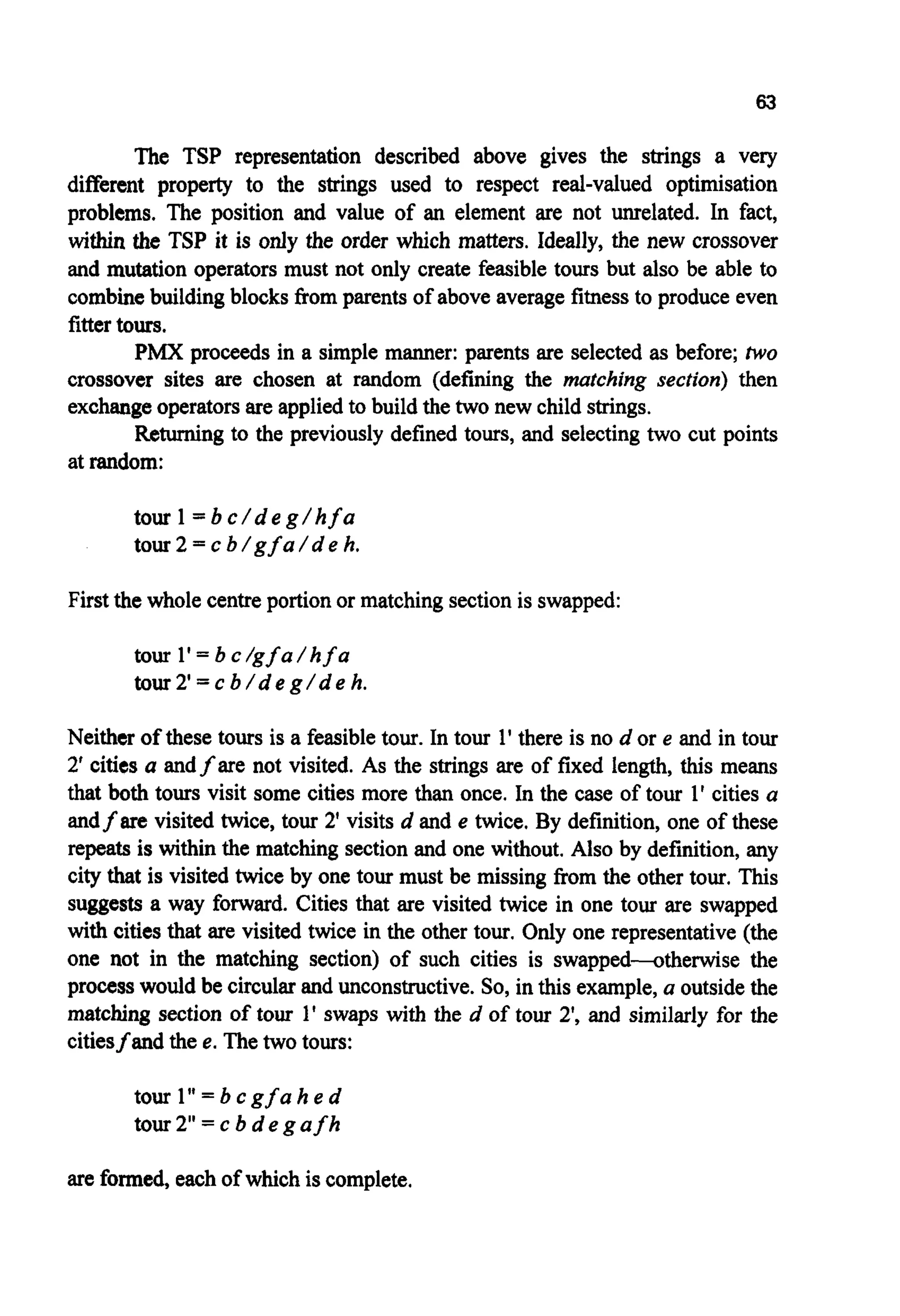
82. 65
One reason for attempting such searches can be best explained by an
example. If the problem characterised by the fitness landscape shown in
Figure4.6 was an architectural one, in which x was the angle of a pitched roof
and f the inverse of the financial cost of the construction, then each local
optima take on a significant meaning. They represent good, but not ideal,
financial solutionsof radically different form. If cost is the only criterion, then
angle x* is the only choice; however if any of the solutions XI, x2 or x3 are
deemed to be more in keeping with other, visual, desires then the architect
might be able to convincethe clientto invest the small amount of extra capital
required. Althoughthere are many points closeto the global optimumthat offer
better values offthan any of the local optima, their closeness to the global
optimum may produce littlejustificationfor adopting such a design rather than
the optimum.This is not so for those structuresrepresentedby the local optima.
In essence,the optimiser is being used as a filter, a filter charged with
the taskof findinghighlyperforming,novel solutionsto the problem across the
wholeproblem spaceand ignoring,asmuch aspossible, all otherpoints.
One way of finding such optima is simply by the use of multiple runs.
Beasley et. al. [BE93a,MI94,p176] indicate that if all optima have equal
likelihoodof being discoveredthenH shouldbe set by:
where p is the number of optima. As all optima will not generally be equally
likely to be discovered,
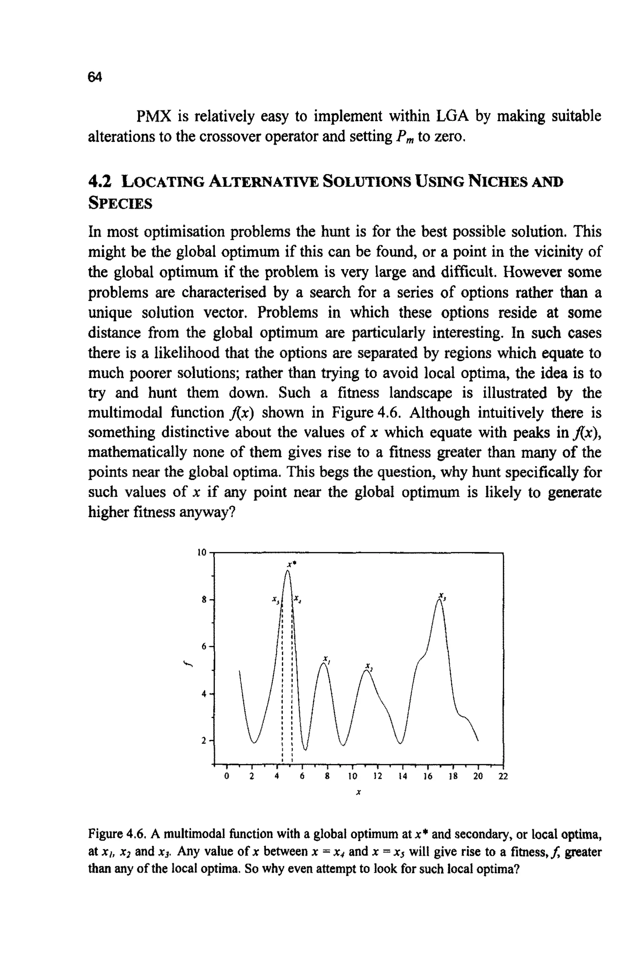
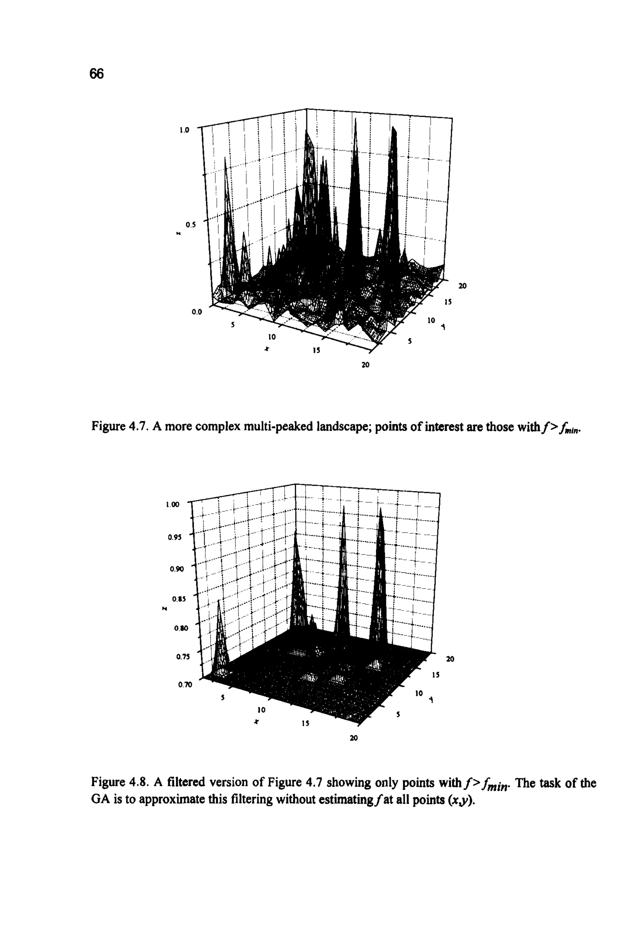
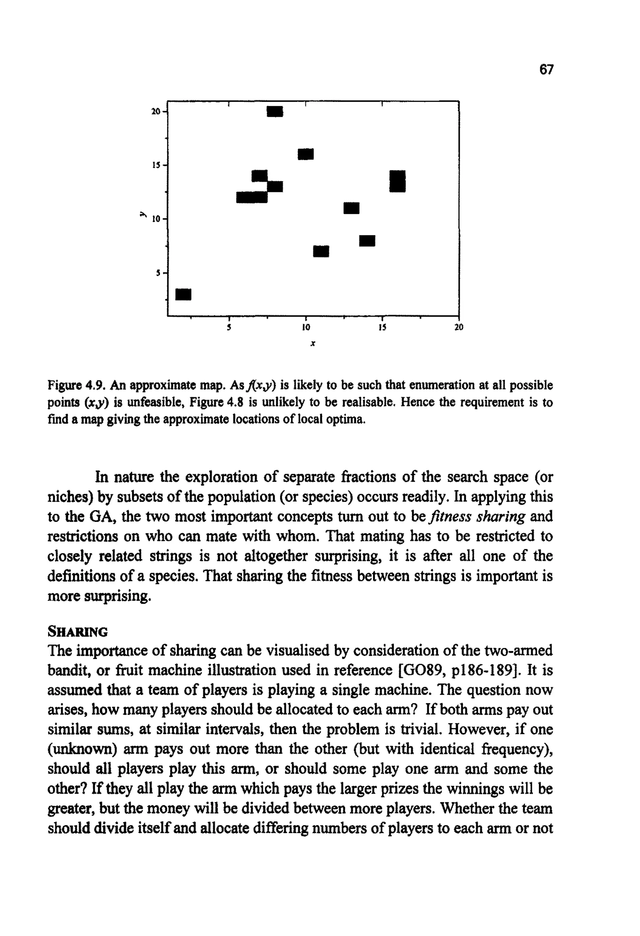
Figure4.7 shows a more complex search space. The quest is for a
technique that can effectively filter out any points that generate a fitness less
than some minimum&,".Such a filter would, if perfect, generate Figure 4.8,
which is much easier to interpret than the original function. In the figures
shown, this filteringis easy to apply by hand because the value off is known at
every point (x,y) within the problem space. Ordinarilyf is likely to be far too
complexto be estimated at more than a small fraction of the search space. So a
technique is needed that can hunt for peaks within a complex landscape
(producing Figure4.9). This is somewhat ironic; up until now the central
consideration has been the avoidance of local optima, now the desire is to
activelyseekthem.
will typicallyneed to be much greaterthan this.

84. 67
L , I I I
s 10 15
Figure 4.9.An approximate map.AsffxJlf is likely to be such that e n ~ e ~ t i o nat a11 possible
points (xy) is unfeasible, Figure 4.8 is unlikely to be realisable. Hence the requirement is to
fmd amap givingthe approximatelocationsof local optima.
In nature the exploration of separate fractions of the search space (or
niches) by subsetsof the population (or species)occurs readily. In applyingthis
to the GA, the two most important concepts turnout to befitness sharing and
restrictions on who can mate with whom. That mating has to be restricted to
closely related strings is not altogether surprising, it is after all one of the
definitionsof a species. That sharingthe fitnessbetween stringsis important is
more surprising.
SHARING
The importanceof sharingcan be visualised by considerationof the two-armed
bandit, or fruit machine illustration used in reference EG089, p186-1893. It is
assumedthat a team of players is playing a single machine. The questionnow
arises,how many players should be allocatedto each arm? If both armspay out
similar sums, at similar intervals,then the problem is trivial. However, if one
( ~ 0 ~ )arm pays out more than the other (but with identical ~e~uency),
should ail players play this arm,or should some play one arm and some the
other? If they all play the arm which pays the largerprizes the winnings will be
greater, but the money will be dividedbetweenmore players. Whetherthe team
shoulddivideitselfand allocatedifferingnumbers of playersto eacharm or not

85. 68
depends on how any winnings are divided,or shared, between the team. If it is
simply a free-for-all,or the winnings are carved up equally between all team
members at the end of the evening, then all the players will migrate to
whichever arm is slowly discovered to be better. However if a rule exists that
monies should only be divided between players of the same arm, then a
different behaviour will emerge. Migration will still occur to the better arm but
after a while those playingthe less good arm will learn that, although they win
less as a group, they gain more individuallybecause there are less members to
share the winnings between. In short, they will have discovered that it makes
senseto exploit a niche.
The ratio of team members playing each arm is easy to calculate. If
there are 25 members in the team and armA pays €50 and armB €40,then if all
players play on A they will receive €50125 = €2 each on a pay-out. If they play
B they receive €40125 = €1.60 each; whereas, if a s&& member decided to
play B they would receive €4011 = €40. This is a very good incentiveto desert
A. A balance will occur once the individualpay-out from each arm is identical.
This will occurwhen
Payout, Payout,
MA m5
-- --
where mi is the number of playerson armj.In this illustrationthis will be when
€50 €40-=-
mA mR
As
mA+mB=25
substitutiongives
50 40
25-m, mg
-----.=-
or
-11.1m3 =--
40x25
50+40

86. 69
and therefore,
mA=25-1 1.1=13.9
With this split between the two arms, the pay-out will be €3.60 each,
greater thanthe €2.00 each would receive if they all playedA.
So,the introductionof sharing allows differentniches to be exploitedto
the benefit of all. Different sub-populations, or species, exploit these niches,
with the number of individuals within a niche being proportional in same way
to the fitness of the niche. If this result could be generalised to other problems a
powerful optimisation approach will have been developed.Not only would the
filtering and mapping of the local optima describedearlier have been achieved,
but the number of individuals exploring any single peak would be proportional
to the height of the peak. This seems a sensible approach as it will ensure the
global optimum will still receive more attentionthan a minor local optimum. In
order to develop these ideas further, the meaning of the term species in this
context will have to be clarified.
SPECIES
In the natural world mating rarely occurs across species boundaries. So far, the
genetic algorithms considered have had no restrictions on who can mate with
whom. That there might be advantages, for some problems, in introducing
restrictions can be understood by considering how a single point crossover
might proceed in the search space shown in Figure 4.10.
If this function is mapped to a binary 4-bit string then -1 = 0000 and
1= 1111. These values both have maximum fitness v(x) = l), and thus one
would expect any selection system to frequently pick them to mate.
Unfortunately,such crossoverswill often generatevery sub-optimalstrings.For
examplethe crossover,
oo/oo
11/11
produces
0011
1100
and

87. 70
as children. Neither of these is anythingnear optimal. In general, in a complex
landscape, matings between distant, well performing, individuals will
frequently produce poor offspring. There might therefore be some benefit in
ensuringthat only like mate with like.
Figure 4.10.The production of sub-optimalsolutions from the crossover of highly performing
strings.
Goldberg and Richardson [GO871 introduced the idea of using a
phenotypic-based sharing mechanism to re-allocate fitness within the
population. The method makes use of a sharing function. This functionis used
to reduce the fitnessof individuals who have a large number of closerelations
(phenotypically)within the population. This limits the uncontrolled growth of
any particular species within the population; it also encouragesthe exploration
of the whole of the search spaceand allows small ~pulationsof i ~ d i v i d ~ sto
reside in any local optima discovered. The value of the sharing function sIfox
an individual i depends on a sum of sharing values tg,between the individual
and allotherpopulationmembers:

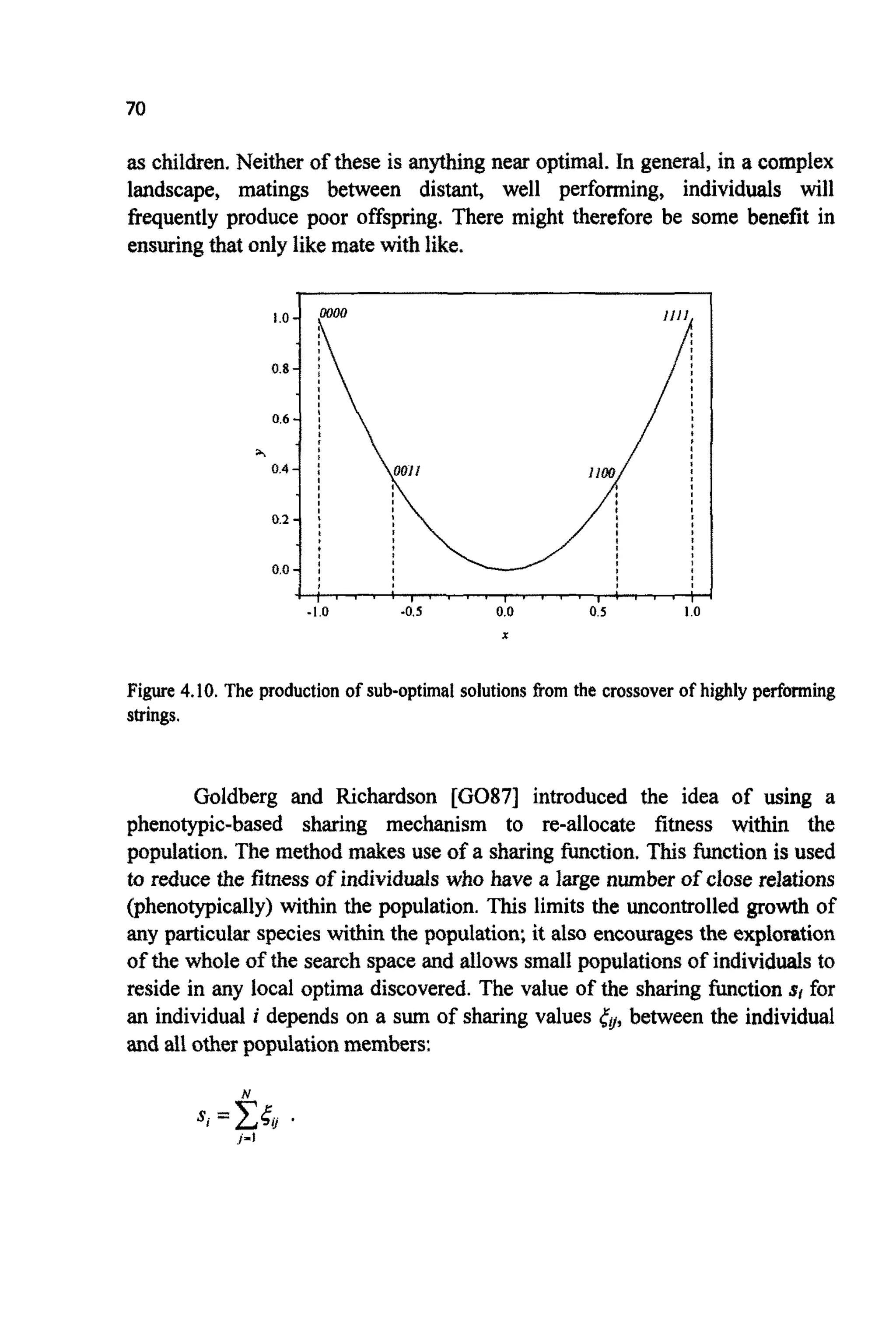
88. 71
The value of r& itself depends on the phenotypic distance between the two
individuals i andj. Several possibilitieshave been suggested and Figure4.11
illustratesone possibility.
I
Figure 4.I 1. One possible sharing function.The distance duis given by the absolute difference
between the two phenotypes in this one parameter problem-the maximum difference being
unity.(After [GO89andG089aI).
The method is implemented by t e m p o ~ l yreducing the fitness of each
individualtemporarilytofskore, givenby:
A successfidapplicationof the techniquehas been the work of Waiters,
Savic and Halhal [HA971 who have used sharing with multi-objective
problemswithinthe water industry(see g6.8).
As mentioned earlier, if lethals are to be avoided then some form of
restrictions on mating may be required [H071,DE89]. Alternatively, in a
similar manner to sharing, Eshelman and Schaffer [ES91,ES9la] bar mating
between similar individuals in an attempt to encourage diversity. Yet another
possibilityis to only allow fit individuals, in particular the elite member, to be
picked once by the selection mechanism in order to slow convergence.
~ ~ f o u ~in [MA95], comparesseveraf nichingmethods.

89. 72
4.3 C O N S T ~ ~ T S
Constraints can been visualised as giving rise to regions of the search space
where no natural fitness can be assign. Such regions produce "holes" in the
fitness landscapes (Figure 4.12). The question then arises of how to steer the
GA around such holes. Lightly constrained problems pose few difkulties for
GAS: the chromosome is decoded to a solution vector, which is in turn used
within the problem to evaluate the objective function and assign a fitness. If
any constraint is violated the fitness is simply set to zero.
"."
Y-1.0
Figure 4.12. A fitness landscape with three large holes caused by the presence of constraints
within a two-dimensionalproblem.
Although attractive, this approach is unlikely to be successkl for more
highly constrained problems (see [MI911 for some ideas). In many such
problems the majority of possible solution vectors will prove to be infeasible.
Even when this is not so, infeasible solutions may contain much usefbl
info~ationwithin their chromosomes. An alternative approach is to apply a
p e ~ l ~ ~ ~ c t i o ~[FCI89] to any solution that violates one or more constraints.
This function simply reduces the fitness of the individ~l,with the amount of
reductionbeing a functionof the violation.
The form of the penalty function must be chosen with care to maintain
the correct balance between exploitationand exploration.

90. 73
A W e r approach is the use of problem dependent crossover and
mutationoperatorswhichdo not allowthe formationof infeasiblesolutions,for
example the crossover operator introduced at the beginning of this chapter
when discussingc o m b i ~ ~ o ~ a loptimisation.
Anotherapproachis illustratedin the work of Walters, SavicandHalhal
[HA971 where a messy GA [G089a,G091a,G093] is used to build
increasingly complex solutions from simple solutions that are known to be
feasible(see $6.8).
In reference [PE97] Pearce uses a technique based on fizzy logic to
resolve c o n s ~ n t swithin a GA environment and discusses constr~nt
resolution in general, Powell and Skolnick, in [PO93], and Smith and Tate, in
[SM93], make general comments on non-linear constraints and penalty
~ c t i o n srespectively. Reference [MI95J discusses the strengths and
weaknessesof severalapproaches.
4.4 MULTICRITEIUAOPTMSATION
The optimisation problems considered so far have been expressed in a form
where, ~ ~ o u ~many parameters might be being optimised in parallel, the
fitness of any particular solution can be specified by a single number, Not all
p ~ b ~ e m sshare this a ~ b u t e ,In some problems the success of a p ~ c u l a r
solutioncan be estimated in more than one way. If these estimationscannot be
combined,then a single measureof the fitness will be unavailable.
An example might be an attempt to minimise the cost of running a
chemicalplant: some of the possibleoperational strategiesfor the plant which
reducethe financialcost of productionmight have the side-effect of increasing
the likelihoodof accidents. Clearlythese solutionsneed to be avoided,whilst at
the same time minimising the production cost in so far as practicable. Most
importantly,solutionswhich are simultaneouslybetter at minimisingcosts and
reducing accidents need to be identified. The concept of Pareto o ~ t ~ ~ a
[GO891can be used to identifysuch solutions. Figure4.13 shows six possible
strategiesforoperationofthe fictitiousplant.

91. 74
4
2
8
I 2 -
‘T
0
0
C
r
b
d
i
I I I
0 2 4 6
Figure4.13. Six strategiesfor the operation of a chemicalplant.
Solution a is optimal in terms of cost; f i n terms of number of accidents.
Solutions c and e are termed dominated because other solutions can be
identified that simultaneously offer both fewer accidents and reduced cost,
these are the nondominated solutions.
If estimationsare made for a large number of operational strategiesthen
the scatter plot of the outer points might take on the form of Figure4.14.
The Pareto optimal set is then the set of all nondominated solutions on
the inner edge of the scatter. Having identified this set (or the equation of the
curve, or front,joining them) it is up to the management and workforce of the
plant to settle on a particular strategy,drawn fromthis set.
Pareto optimalitycan be used in at least two ways to drive a rank-based
selection mechanism within the GA. Nondominated sorting [SR94] identifies
the Pareto optimal set and assign all members the rank of 1. These individuals
are then removed from the ranking process. The next optimal front is identified
and its members given the rank of 2. This process is repeated until all
individuals have been ranked. BASIC code to carry out this procedure is given
in Figure 4.15 and the approach is demonstrated in $6.8. An alternative
approach is the Pareto ranking scheme of reference [FON93] where rank is
proportional to the number of individuals that dominate the individual in
question (Figure 4.16).

92. 75
20
I
0 5 10
cosr
I5
Figure 4.14. Surfaceformed fromall possible strategiesfor the chemical plant's operation(only
the outer points are shown). The Pareto optimal set (or tiont) is formed from the nondominated
solutions.
FOR i R a n k = 1 TO N 'Loopover all possibleranks.
I F Rank ( i) = 0 THEN 'Only processunranked individuals.
FOR i = 1 TO N 'Pickan individual.
FOR j = 1 TO N 'Loop overall other individ~ls.
I F i <> j THEN 'Check fordomination.
END I F
IF F l ( i ) < F l ( j ) AND F 2 ( i ) < F2(j) THEN EXIT FOR
NEXT j
I F j = N t 1 THEN R a n k ( i ) = i R a n k 'Anondominatedsolutionh~
END IF 'been identified
NEXT i
FOR i - 1 TO N 'tozero.
Wow removethe currentnondominated frontby settingthe fitnessof individualson the front
I F R a n k ( i ) = i R a n k THEN
F l ( i ) = 0
F Z ( i ) = 0
END I F
NEXT i
NEXT i R a n k
Figure4.15.Nondominatedsorting(continuesover).

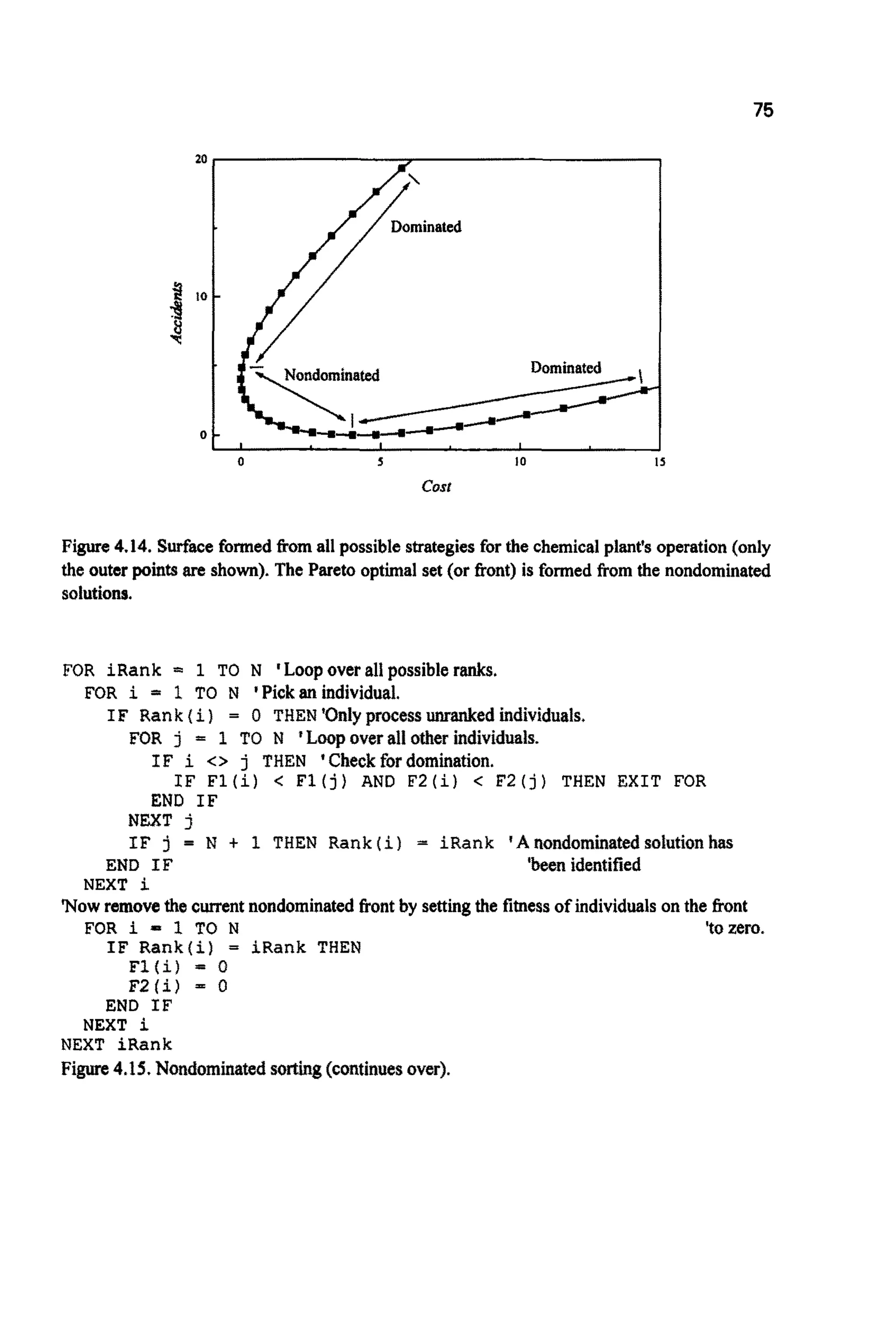
93. 76
FOR i = 1 TO N 'Re-assign fitness basedonrank
NEXT i
Figure 4.I5 (continued).BASIC code to cany out nondominated sorting of a population of size
N.The problem contains two measures of fitness, F1 and F2, which are reduced to a single
measure F by letting F =l/Rank.
F ( i ) = 1 / Rank(i)
6
5
4
5
3
2
1
1 2 3 4 5
rank 4
1"7
Figure 4.16. Pareto ranking for a problem of two criteria giving rise to two fitness functionsfi
mdh.
Both techniques require the use of fitness sharing to ensure that the
population covers a large enough fraction of the search space [HA97]. (See
[GR97] for some recent ideas about this).
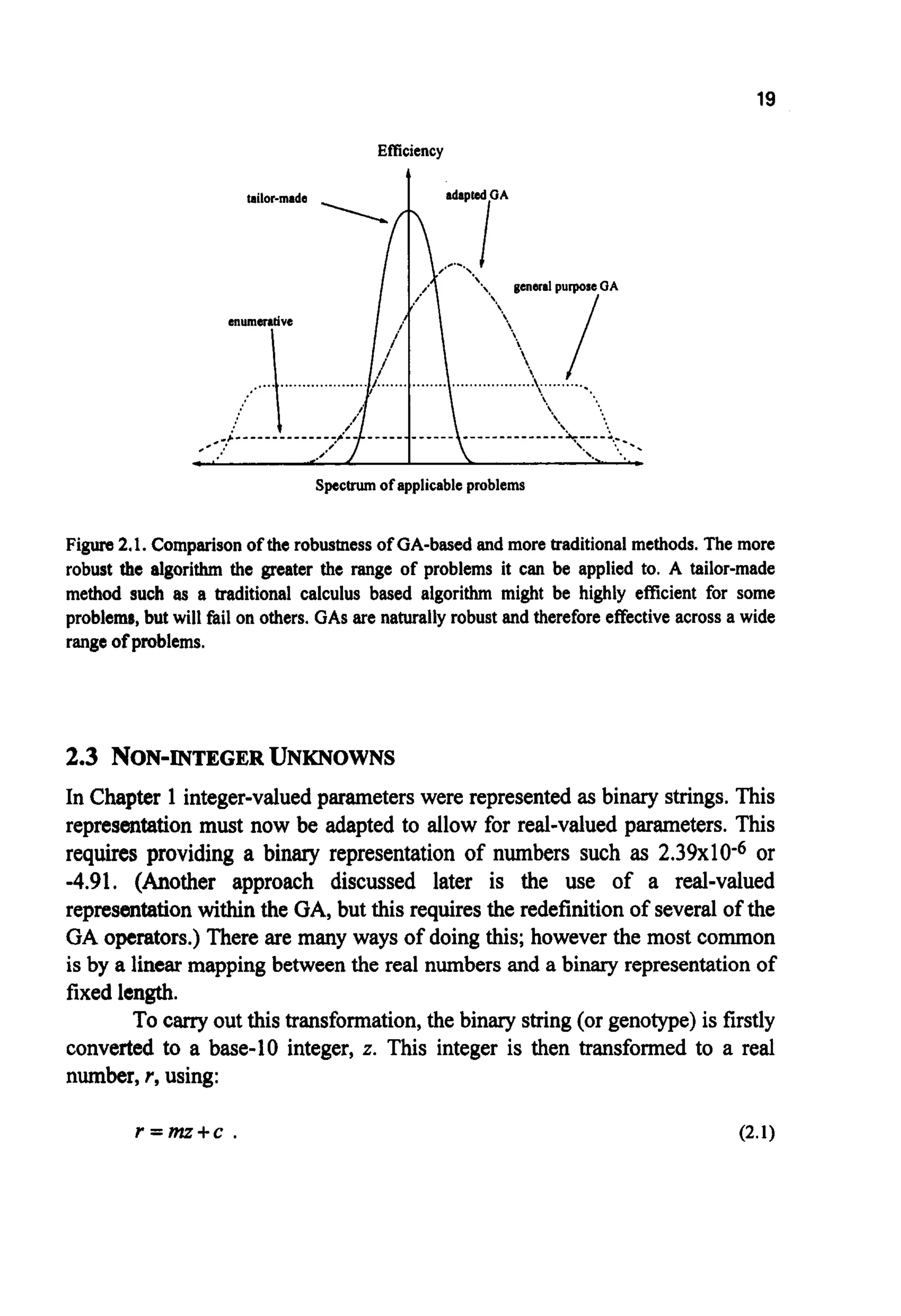
4.5 HYBRIDALGORITHMS
Genetic algorithms are not very good at finding optimal solutions! However
they are good at navigating around large complex search spaces tracking down
near-optimal solutions. Given enough time a GA will usually converge on the
optimum, but in practice this is not likely to be a rapid process. There are many
other, more efficient, traditional algorithms for climbing the last few steps to
the global optimum. This implies that a very powerful optimisation technique
might be to use a GA to locate the hills and a traditional technique to climb

94. 77
them. The final a l g o ~ ~will depend on the problem at hand and the resources
available.
The simplest approach to this hybridisation is to use the real-valued
solution vector, represented by the fittest individual in the final generation, as
the startingpoint of a traditionalsearch. The traditional search algorithmcould
be either a commercial compiled one, such as a NAG routine, or taken Erom a
text on numericalmethods.
Another, approach is to stay with the string representation used by the
GA and attempt to mutate the bits in a directly constructive way. One way to
achieve this is illustrated in the estimation of the ground-state of a spin-glass
presenbd in $6.4.In this example, local hills are climbed by visiting each bit
within the string in turn,mu~tingits value and re- valuating the fitness of the
population member. The mutation is kept if the fitnesshas improved.Another,
very simple, possibility is to hill-climb by adding (or subtracting) I to the
binary representation of the first unknown parameter in the elite string (e.g.
1101 + I = lllO), re-evaluating the fitness, and keeping the addition
(subtraction)if it has proved beneficial. This addition (subtraction) is repeated
until adjusting the first unknown parameter shows no benefits. The other
parametersare then treated in the sameway.
Working with the GA strings themselves has the advantage that such
techniques can be applied at any moment during a genetic algorithm's run.
Moving to a real encoding can make it difficult to return to a binary string
represented GA, because some parameters may have taken values that can not
be represented directly by such a string (see Chapter2). However, such real-
valued methods are typically highly efficient. One way around this problem is
not to use a binary stringrepresentationwithin the GA (as discussedin $4.7).
If the search space is believed to be complex at many scales,
abandoning the GA in favour of another method too soon can lead to an
erroneous solution. The liquid crystal problem studied in 56.5 contains just
such a space. In this work, using the final solution vector as the starting point
for a more constrainedGA-based searchwas foundto be effective.
Other methods of improvingperformanceand convergencespeed make
use of heuristics. One such example is the use of inter-ci~distanceswithin a
TSP(i.e, makingit no longerblind). Grefenstetteet, al. used this informationto
produce an improved uniform-type crossover operator. Rather than building
child strings by taking alternating cites from each parent, the child inheritsthe
city which is geographicallyclosest to the current city [GR85].
Alternatively, the fitness evaluations-which are typically the most
time consuming element of the algorithm4an initially be done in an

95. 78
approximate manner (see $6.5). For example, in problems which use least-
squares minimi~tionof experimental data, this can be achieved by initidly
only presenting the GA with a random, regular or other subset of the data and
running a fixed number of generations. The initiallysubset is then enlarged to
include more of the data and further generations processed [MIK97a]. This
process is repeateduntil all the data isWing considered.
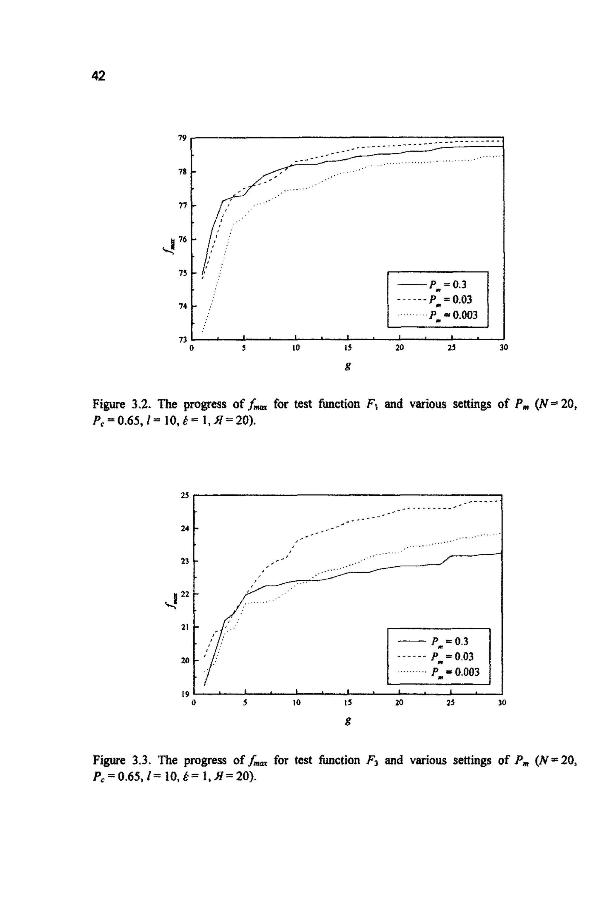
4.6 ALTERNATIVESELECTIONMETHODS
The selection pressure within the GA is centrai to its performance, and the
appropriate level is highly problem dependant. If the population is pushed too
hard, rapid progression will be followed by near stagnation with little
progression i n f , This is unsurprising. With a high selection pressure the
population will become dominatedby one, or at most a few, super-individuals.
With very little genetic diversity remaining in the population, new areas of the
problem-space become machable-except via highly unlikely combinations
of mutations. Another way of visualising the effect of this pressure is by
consideringhow directed the mechanism is toward a sub-set of the population
( ~ i c a l l ythe best). Highly directed m e c ~ s m swill result in a p a t h ~ ~ ~ n ~ t
search,less directedmechanismswill result in a volume-orientatedsearch.
The selection pressure can be characterised by the take-over time, r
[G091]. In essence, this is the number of generations taken for the best
individu~in the initial generation to completely dominate the pop~&tion.
(Mutation and crossover are switchedom. The value of f depends not only on
the selection mechanism, but for some mechanisms, on the function being
optimised.If fitness proportionalselection is used, then for:
1
a
f ( x ) =xa, f =-(Md-1)
and for
1
a
f(x)=exp(ax), f=--MnN
[GO9l,BA96,pl68], i.e. of the generalorderMnN.
Other selection mechanismsare common (see [G091]) and in essence
they all try to encouragethe GA to walk a fine tight-rope between exploitation
and exploration,whilst minimising sampling errors. Such mechanisms usudily

96. 79
make the assumption that if a individual has a lower fitness, it is less likely to
be selected. Thisneed not be so, as Kuo and Hwang point out in [KU93].
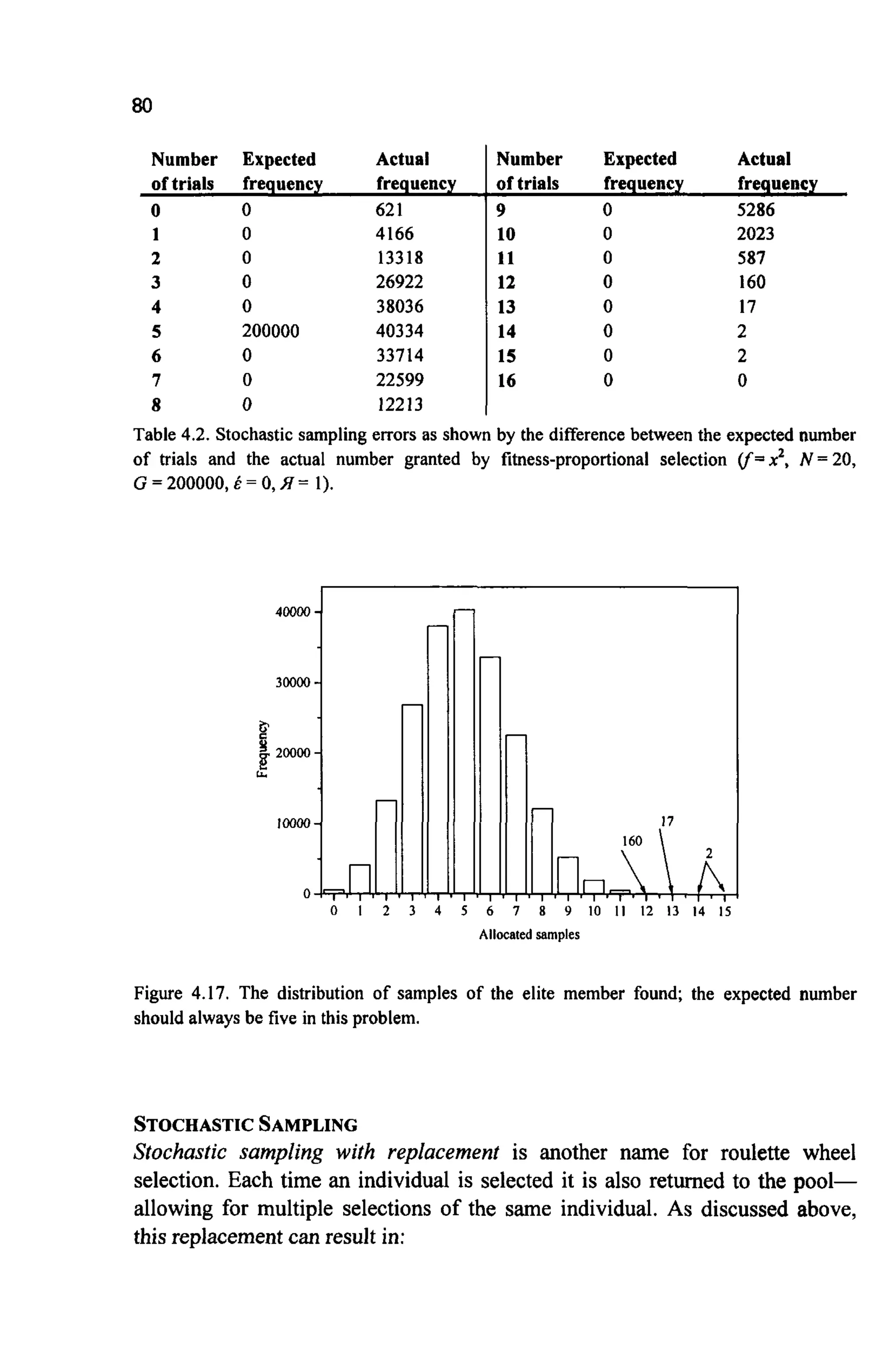
STOCHASTICSAMPLINGERRORS
Fitness-proportional selection is a stochastic method. On average, the number
of trials,q,(inthe next generation)an individual,i, is given will be suchthat if
then
r, =2raw
where rp" is the numberof trials an individual of averagefitnesswould achieve
(typically 1). This number will not always be achieved. GAS make use of
numerous calls to random number generators, and given enough calls, some
surprising patterns can emerge. Table4.2 and Figure4.17 show the result of
using the roulette wheel algorithm in LGADOS for N =20 and G = 200,000.
The results are for the elite member which, because of the problem used, has
j7g)= 5fm(g) for all g, and should thus have on average five trials in the next
generation. Although five is indeed the most common number of trials
allocated, many other possibilitiesalso occur. On 621 occasions no trials were
allocated to thisthe fittest member. This implies that, unless elitism is in place,
the best solution would be discarded. Converselyfmarwill occasionally almost
flood the population. Such over or under selection can greatly impair the
performance of the algorithm, and a number of alternative selection methods
have been designedto minimisethe problem.

97. 80
Number Expected Actual
of trials frequency frequency
0 0 621
1 0 4166
2 0 13318
3 0 26922
4 0 38036
5 200000 40334
6 0 33714
7 0 22599
8 0 12213
Number Expected Actual
of trials frequency frequency
9 0 5286
10 0 2023
11 0 587
12 0 160
13 0 17
14 0 2
15 0 2
16 0 0
40000
30000
P
g20000
L*
10000
0
0 i i 3 4 6 i i 9 i o I i i 2 1 ' 3 i i i s
Allocatedsamples
Figure 4.17. The distribution of samples of the elite member found; the expected number
should always be five in this problem.
STOCHASTICSAMPLING
Stochastic sampling with replacement is another name for roulette wheel
selection. Each time an individual is selected it is also returned to the pool-
allowing for multiple selections of the same individual. As discussed above,
this replacementcanresult in:

98. 81
(the expected number of trials for individual i). Stochastic sampling without
replacement forcesthe maximum number of trials an individual can receive to
equal unity (by not returning selected individuals to the pool). This is a major
brakeon the selection mechanism. However, it does still allow zbesf,the number
of trialsallocatedto the fittestindividualto equal zero occasionally.
Remainder stochastic sampling (with and without replacement)
estimatest;"p(g) then sets:
whereINT(-)returnsthe integerpart of (-).
In general this will leave some slots in the new population unfilled.
Stochastic sampling with replacement is then used to fill the remaining
positionsby usingthe fractionalparts.
to assign roulettewheel slots.
random number R', between 0 and 1. An individualis selectedif:
The method can also be used without replacement by simply using a
Stochastic universal sampling [BA87] also uses a roulette wheel but
with N equal spaced markers. The wheel is spun only once and all individuals
which falladjacentto a marker are selected.
RANKING METHODS
If the position of an individual within a list ordered by fitness is used to
calculatet i then problems of super-fit individuals are avoided. The position of
the individual within the list is all that matters, not how much fitter than the
population average it may be. This greatly suppresses problems of premature
convergence,whilst stillproviding a suitable level ofselection pressure in later
generations.

99. 82
In its simplest form, the population is ranked and the best 50% of
individuals selected to go forward to the next generation. Crossover is then
performed on all selected individuals by choosing random pairs without
replacement.
More subtle methods have been presented [BA85]. One possibility is to
fix rzf by hand and then apply a linear curve through zz$ that encloses an
area equal to N. The height of the curve then supplies rFpfor each individual
(Figure 4.18).One problem withthis approach is the need to selectthe value of
r z ,which will (of course) be problem dependent. Other methods use a non-
linear curve [MI94].
Rank
Figure 4.18. Linearranking.
The take-over time for rank-based selection depends on the details of
how it is applied, in particular on the value of z z f ,but ris of the order InN,
i.e. much lower than with fitness-proportional selection [GO91,BA96,pl71].
TOURNAMENTSELECTION
Tournament selection [GO91,BL95] is both effective and computationally
eficient. Pairs of individualsare selected at random and a random number, R'
(in the range 0-1) generated. If R+>r, 0.5 <r 5 1, then the fitter of the two
individualsgoes forward, if not, the less fit. The value of r also requires setting
by hand.

100. 83
In other imp~e~entatio~q individ~~sare i ~ t i ~ I yselected with the
singlebest goingthroughto the next generation.Suchanapproachhas:
This implies that the takeover time will rapidly decrease as q moves away
from2 (Le.binary tournaments).
SIGMASCALING
Linear fitness scaling {C~apter3)can be extended by making use of the
pop^^^ fitness standard d e ~ a t i o n ~ ~[MI96], with the expected number of
trials givenby:
STEAKWSTATEALGORITHMS
LOA is agenerationalalgorithmin that at each generation, a new populationis
formed (although some will be direct copies of their parents not disrupted by
crossovm or mutat~on)~Steady-state a I ~ ~ ~ ~ s[SY89,SY9€,W~89,DE93a]
replaw only a few of the ieast fit i n d ~ v i d ~ seach g e n ~ ~ t ~ o ~by c ~ s s o v e ~and
mut&ioG and thus require few fitness evaluations between generations, The
fractioa of individuals replaced is called the g ~ ~ ~ ~gap fDE75J. Such
go^^ have provedhighly effectiveon problemswhere identicalgenotypes
alwaysreturnthe samevalueofffor all esti~ations(thiswill not necessarilybe
so withnoisy, timevaryingdata) [DA9l],
4.7 ALTERNATIVECROSSOVERMETHODS
Single point crossover has been criticised for several reasons [CAW, ES89,
SCSSa]. Although it can recombine she% low-order, schemata in
a d ~ ~ g ~ u sm ~ e ~ ,it ~ ~ e n t l ~cannot process all schemata in the stme
way. For example,given:
~~O####Iand
###00###,

101. 84
single point crossover cannot form
01000##1
Such positional bias [ES89] implies that schemata with long defining lengths
suffer biased disruption.
Crossover of strings that are identical to one side of the cut-point will
have no effect, as the children will be identical to the parents. The reduced
surrogate operator [B087] constrains crossover so as to produce new
individuals wheneverpossible. This is achieved by limiting cut-points to points
where bit values differ.
TWO-POINTCROSSOVER
In order to reduce positional bias, many researchers use two-point crossover
where two cut points are selected at random and the portion of chromosome
between the two cuts swapped.For example:
00/0100/111and
11/101UOOO give
001011111and
I10100000.
Just as with single point crossover, there are many schemata which two-point
crossover cannot process, and various numbers of cut points have been tried
[EC89].
UNIFORMCROSSOVER
Uniform Crossover [SY89] takes the idea of multi-point crossover to its limit
and forces an exchange of bits at every locus. This can be highly disruptive,
especially in early generations.Parameterised crossover [SP911moderatesthis
disruption by applying a probability (typically in the range 0.5-0.8) to the
exchange of bits between the strings. (For a discussion of multi-point crossover
see [SP91b]).
4.8 CONSIDERATIONS OF SPEED
In most practical applications, the time taken to estimate the objective
functions,Q, will be greatly in excess of the time taken to cany out any genetic

102. 85
operations. Thereforethere is little need to worry about trying to time-optimise
these operations. One way to ensure minimum runtimes is to try and speed the
estimation of Sdxg). Two possibilities are to interpolate from pre-existing
values, or to use an approximate value of Sat&) for some generations but not
others. This could be by using the approximationforg <g’then revertingto the
true estimation for g2 g‘.This approach is used in $6.5, when only a sub-set of
the experimentaldata is used in early generations.
An obvious but important possibility is to ensure that Q(g) is not re-
estimatedonce it has been found for a particular chromosome. This will require
maintaining a (possibly ordered) list of all values of Sa calculated during the
run.Clearly, this list has the potential to become extensive and it might be of
value to only store it for g- 1 to g -k,where the historic period k used will
depend on the relative time overhead of examining the list and estimating
another value of 0.If new estimates are placed at the bottom of the list, it will
probably prove worthwhile to search the list in reverse order to maximise the
gain (see56.6).
A further possibility is to use a network of computers to carry out
separateestimatesof Q(g)on separatemachines.
In addition to all of these considerations, it is necessary to ensure the
use of the minimum values of 4 (j= 1...M) and to keep the range of values
each parameter can take as small as possible. Both the range and the string
length can be functions of generation (see $6.5) but care must be used as this
effectively removes areas of the search space during certain generations.
Alternatively a messy-GA [G089a,G091a] can be used to build complex
solutionsfrom simplebuildingblocks (for example, 56.8).
4.9 OTHER ENCODINGS
This text has concentratedon binary encoded GAS. Many authors have pointed
out that GASwill probably be at their most effective when the encoding is as
close as possible to the problem space. For many problems in science and
engineering this implies the use of numbers of base-10 form. Unfortunately,
using a real-valued encoding poses a large number of questions; in particular,
what to use as crossover and mutation operators. Several possibilities have
been promoted and a detailed discussion is to be found in references [MI94],
[ES93], [JA91] and [WR91]. Reeves in [RE931 makes comments on the
implicationsfor population sizes of using non-binary alphabets.
One possibility for crossover (between individuals i and k) is to use
[MU93,ZA97, p14-161:

103. 86
where R is a random scalingfactor(typicallyin the range-0.25 to 1.25).
Mutationcan be includedin several ways, for example:
r,(g+I)=r;(g)+R*(g)r,(g);R(g=O)=R*,R(g) 3 O a s g 4 G
Things need not however be made too complex and a binary
representation will often work extremely well. As Goldberg has pointed out
[G089,p80], GAS are typically robust with respect to the encoding used. He
givestwo simplecodingrules:
1. The Principle of Meaningful Building Blocks: the user should select a
coding so that short, low-order schemata are relevant to the underlying
problem and relativelyunrelatedto schemataover other fixedpositions.
2. The Principle of Minimal Alphabets:the user should select the smallest
alphabetthat permits a natural expressionof the problem.
It is relativelyeasy to get someidea of why the use of a binaryencoding
is a reasonable choice for many problems. Consider some of the strings that
might occur when solving fix) =x2 , 0 I x 5 15 with either a 4-bit binary
presentation or a one-to-one mapping of binary integersto the first 16 letters
of the alphabet. Table 4.3 shows five possible values of x together with their
respective binary and non-binary strings. As the list is descended, there is an
obvious visual connection between the binary stringsof fitter individuals made
possible by their low cardinality (number of distinct characters): they all have
1’s toward the left-hand side of the string. In the non-binary case no such
similaritiescan exist. As these similaritiesare at the heart of the searchmethod,
their numbershould be maximised.
Another way to emphasise the difference is to count the number of
schemata available in the two representations. For cardinality k, this will be
(k+ As the same accuracy is required from both encodings, L =4 in the
binary case and 1 in the non-binary case. Therefore, the binary repr~sen~tion
contains (2 + 1)4 = 81 schemata and the non-binary (16 + 1)’ = 17 schemata(a
to n plus #), a clear advantageto the binary representation.

104. 87
X f C(binary) C(non-binary)
1 1 0001 a
2 4 0010 b
3 9 0011 c
12 144 1100 I
14 196 I110 m
Table 4.3.Comparisonof binaryand non-binaryrepresentations.
LOGARITHMICREPRESENTATION
For many scientific and engineering problems, it is only the relative precision
of the unknownswhich is important [ZA97]. In such cases the encoding of the
logarithm of the unknown may prove more suitable. This will allow a very
large space to be searched without the need for excessive string lengths, but
still maintain reasonable accuracy when needed. For example, if an unknown,
r, may take any value between 1and 1,000and the answer is required to 1part
in 100,then a simple linear mapping between the problem space and a binary
representation requires adjacent points to vary by only 1/100= 0.01, This will
then allow values of r around 1to be distinguishedto the required accuracy of
1%. However, the precision around r = 1,000 will still be 0.01, which is 1part
in 100,000or 0.001%. This impliesthat most of the stringis redundant.
By using a logarithmic mapping the required accuracy can be
maintained throughout the space with a much shorter string,thereby enhancing
performance.
GRAYENCODING
It was suggested above that a GA might be at its most successhl when the
encoding used is as close to the problem space as possible. Thus, a “small”
change in the phenotype should indicate an equally “small” change in the
genotype. For a binary encodingthis is not so. Given a genotypewith I = 6 and
a phenotype,r with 0 Ir I63then
011111= 31
will have to undergo changes to all six bits to increase the value of the
phenotypeby one:
100000= 32.

105. 88
Binary Gray
0000 0000
0001 0001
0010 0011
0011 0010
0101 0111
0110 0101
O I I l 0100
0100 aiio
Gray binary encodingalleviatesthis by ensuring that any pair of adjacentpoints
in the problem space differ by only a single bit in the representation space.
(Note, a small changein the genotypecan still lead to a very large changein the
phenotype). For many problems this adjacency property is known to improve
performanceand it would seemsensibleto adoptthe use of a Grayencodingfor
most problems with integer,real or complex-valuedunknowns.
Table4.4 list binary and Gray equivalentsfor 1= 4. Figure4.19 presents
BASIC code for converting Gray to standard binary; reference [ZA97, p96]
givespseudo-codefor carryingout this ~ansfo~ation.
Binary Gray
1000 I100
1001 1101
1010 I l l 1
1011 Ill0
1100 1010
I101 1011
1110 1001
1111 I000
Bin(1) = Gray(1)
FOR i = 2 TO L
Bin(i) = 0
Bin(i) = 1
IF Bin(i - 1) = Gray(if THEN
ELSE
END IF
NEXT i
Figure 4.19. BASIC code to convert Gray to standard binary. The Gray and binary strings,
Gray and Bin (each oflength L) are assumed to be held in arrays where the first element is
the most significant.

106. 89
4.10 METAGAS
Much has been made in this text of the need to choosethe internalGA settings
(Pc,P,, N,etc) with care, and of the fact that their optimum settingsare likely
to be highly problem-dependent (as will be the exact form of the algorithm).
This leadsto the very natural question, why not have these settings selected by
a separateGA?Furthermore,asfbst+f* the form of the searchspaceis likely
to change, implying that the ideal internal settings might not be constant in
time. This leads naturally to the possibility of using a GA to optimise the
internalsettingsduring the runitself.
If only a single value of each internalparameter is required, and the GA
is goingto be used repeatedlywith near-identical problems, then the approach
is relatively easy to ~plementby using a meta-level GA [GRS6,BR91] to
controland evolvesettingswithin a populationof GAS.
Howeverin difficultproblems,or wherethe GA will only be used a few
times, the additional computing required probably makes the approach
unrealistic. The abilityto allowthe settingsto adapt in real-time [DA89,DA91],
might however allow the design of extremely eMicient algorithms, and is a
particularlyinterestingavenueof research.
4.11 MUTATION
So far mutation has come in a single guise: the infrequent random flippingof
bits within the c~omosome.Traditionally, mutation has always been seen as
very much a secondarymechanismin comp~sonto crossover. Howeverthere
would now appearto be a growing feelingthat it may have a more centralrole
to play [MU92a,HI95,JO95].
The mutation operator as described in Chapter 1 is rather a blunt
instrument, the main role of which would appear to be ensuring that the
~ p ~ a ~ ~ o nmaintainsboth possiblebit values (0and I)at all loci. If mutationis
to be applied in a more directed manner, i.e. as part of the searchprocess itself,
then it would seem sensible to make the operator more discriminating. For
example, with a binary representation (standard or Gray) the magnitude of the
disruption caused by mutation depends upon where in the chromosome
mutation occurs. Given a single parameter problem with L = 10, rmf,=0 and
r,, = 1023, then a mutation at one end of the chromosome changes Y by *l,
whereasat the otherend r would changeby *5 12.
This analysisindicates that near the end of the run,when hopefully the
majority of the population is in the vicinity of the global optimum, there might
be advantages in confining mutation to lower order bits. Conversely, during

107. earlier generations mutation of the higher order bits will help in the full
explorationof the space,whereasmutationof less significantbits will add little
to this exploration. (See the exercises at the end of this chapter for one
possibility).
Other possibilities are to bias mutation towards less fit individualsto
increase exploration without degrading the performma of fitter individuals
[DA89], or to make P,,, a function of g with the probability decreasing with
generation [F089].
Altem~tively,mutation can be used in a hill-climbing sense to close in
on the final solution after g =G. This is achieved by using mutation to slowly
increase (or decrease) estimates of each unknown within the elite member,
keepingthe changeonly if it has proved constructive(i.e. increasedf,).
See [BA93J and [TA93J for a discussion on setting optimal mutation
rates.
4.12 PARALLELGENETICALGORITHMS
Apart from the implicit parallelism provided by schemata processing, the
population-based approach of GAS makes them ideal for implementation on
parallel, or networked, machines. Althou~,for many, the reason for using a
parallet implementation will be a simple increase in speed due to the increase
in computer power, others use pseudo-parallel approaches that are believed to
improveperformanceeven when used on sequentialmachines.
Global Parallel GAS [G089,HU91,D091] treat the population as a
single unit and assign different individuals to different processors. In its
simplest form, the approach uses one machine (or processor) to control
selection and the genetic operators, and a series of other machines (or
processors) to cany out objective function evaluation. If the objectivefunction
evaluation takes a considerable time, a substantial speed-up can be achieved
given a littleadditionalcodeand a roomful1of personal computers.
~ i ~ a t i o nor Island GAS [TA87,TA89] attempt to mimic the
geographical separation of subpopulationswitnessed in the natural world. This
is achieved by allowing separatesubpopulationsor demes of chromosomes to
evolveusing selectionand crossover,but then allowing occasionalmigrationof
individualsbetweensubpopulations.
D i ~ s ~ o n ,neighbourhoud, cellulur, or ~ n e - g r a i ~ e ~GAS remove the
subpop~ationbarriers used in the migration methodology and replace them
with the conceptof geographicaldistance. Individualsare then only allowed to
breed with closeneighbours [RO87,MA89,SP91a,DA91a,MA93].

108. 91
Parallel GASare introduced in greater detail in reference [ZA97, p20-
301.
4.13 SUMMARY
In thischapterseveraladvancedoperatorshave been introduced,includingones
to tackle selectionand crossover in c o m b ~ t o ~ ~ land multicritiaopt~isation.
The latter leadsnaturallyto the in~ductionof the concept of maintainingsub-
populations of differing species within the algorithm. One possibility for
dealingwith constraints,the penalty function, has been suggested-although in
practiceitsuse is far from straightforward.
Alternative representations have been introduced and the
reco~endationthat if a b i n ~ - ~ erep~sentationis used, then a Gray
encoding is adopted. The use of a logarithmic representation has also been
promoted.
Hybrid algorithms, which combine a GA with a more traditional
algorithm, have been hinted at as a highly powerful combination for solving
practicalproblems.
Alternative selection, crossover and mutation mechanisms have been
discussed, in part to alleviate stochasticsamplingerrors, but also as a way of
ensuring the correct balance between exploration and exploitation. Meta GAS,
where the algorithmitself adapts duringa run,are one way this balance might
be naturaily found.
Finally, parallel a l g o ~ ~have been m ~ t i o n e ~as an interesting
avenueof research.
4.14 EXERCISES
1. W u c e PMX into LGADOS,BAS, or your own GA, and use it to help
solvethe simpleTSP detailedin Table4.1.
2. By includinga subroutineto apply a simplepenaltyfunction,solvea lightly
constrained multi-dimensional problem of your choice. Experiment with
the strengthof the penaltyfunctionto see the effecton the efficiencyof the
~ g o r i ~ .Increase the level and n~~ of ~ n s ~ a i n ~until most of the
search space is unfeasibIe. (This should indicatethat penalty hctions are
possibly inappropriatefor suchproblems.)

109. 92
3. Introduce tournament selection, linear rank selection, two-point crossover
and ~ i f o ~crossover into LGADOSBAS, or your own GA, and study
their effecton test hction performance.
4. Designand implementa new mutation operator,P$,which gives a reduced
probability of mutation of more significant bits during later generations:
PA = P,E(j,g) ;1 Ij II& ,1 Ik IM .The functionBshouldbe linear inj .
Studythe effectof differingfunctionalformson test functionperformance.
5. Convert LGADOS.BAS, or your own GA, to a Gray encoding. (This is
easier than it might seem and only involveschanginghow the binary strings
are converted to integers.) Compare the performance of binary and Gray
encodingon varioustest hctions and variousmutation rates.
6. Allow for a ~ o g a r i t ~ i crepresentation within LGADOS.BAS, or your own
GA. Use the new code to solve MAXV= XI;0 Ix 5 1x106to 1% across all
x and comparethe performanceto a linear representation,
7. Adapt LGADOSBAS, or your own GA, to stop the evaluation of
individuals that existed in the previous generation. Plot graphs of fmm
against number of objective function evaluations for some of the test
functionsof Chapter 3. What effect does this have on the efficiency of the
algorithmfor various settingsof Pcand P,? Extend the approachto stopthe
evaluation of i n d i v i d ~ ~that have occurred in the last ~ - g ~ n ~ a t i o n
(1 Ik 5g>.Use N 2 100in your experiments.

110. 93
CHAPTER5
WRITINGA GENETICALGORITHM
Implementinga genetic algorithm on a computer is surprisingly easy. Much of
this simplicity arises from the lack of sophisticated mathematics within the
algorithm: there are few operations that would be beyond even the most rusty
or inexperiencedof individuals.
For most applications, the programming language chosen for the GA
itself will be of little relevance becausethe majority of computationaltime will
be spent estimating the objective function. Thus it is far more important to
ensurethat that part of the program is optimised in structureand language. As
most programmingenvironmentsallow mixed languageprograms, the GA and
the objectivefunctionroutines need not even be in the same language (or even
d n g on the samemachine).
Althoughthere are several GA packages available,either commercially
or for free, I strongly believe in the value of trying to code one’s own simple
algorithm, at least in the first instance. For experienced programmersthis will
take less than a day.
The implementation described here is of LGADOS and is designed to
run under QBASIC on a PC. BASIC has been chosen, in part, because of its
ease of comprehensionby the less experienced (and because it is included on
most DOS-based systems). Sophisticated data structures have been avoided,
and although this possibly makes the algorithm slightly less elegant, it should
allow for easy translation into any other language (translationsinto PASCAL,,
FORTRAN and C are alreadyprovided on the disk). Those wishing to work in
PASCAL might like to use code from reference [G089]; those with a
preference for C could use the code in reference [MI941 (although this is for a
real-valued, rather than a binary, encodedGA).
This chapter starts by sketchingthe form of the program, explainingthe
data structure adopted, listing the main program and then examining each
operation and its associated subroutine (procedure) in turn. Extracting the

111. 94
results and adapting the program to solve other problems is also discussed.
Although a rough understanding of the program is advisable, it would be
possible simply to make suitable adjustments, as detailed below, and run the
code via QBASIC or a BASIC compiler (QuickBASIC would be ideal) and
solve other, more complex,problems.
A complete listing of the program is included on the disk and in
Appendix B.
A SKETCHOF THE PROGRAM
At the heart of the program are two non-overlapping populations of bmary
encoded strings. One is the current generation, the other a new temporary
population in the process of being constructed from the current generation by
selection, crossover and mutation. When the temporary population is complete
it replaces the current generation and the generational counter is incremented
by one. Thisprocess is sketched in Figure 5.1.
Generation = 1.
Create initial population 'Buildapopulation ofstrings at random.
Find unknowns 'De-codethe n ~ p o p ~ l a t i o nto integersthenreal numbers,
Find fitness Find thefitness of eachmember o~~hepopulation.
FOR Generation = 2 TO maximum number of generations
FOR NewIndividual = 1 TO PopulationSize STEP 2 'Loopoverthe
popula#~onchoos~ngpairsof mates
Select a mate
Select other mate
Perform crossover 'Passindividualsto the temporarypopulation afer
performingcrossover.
NEXT NewIndividual
m t ate
Repface
Find unknowns
Find fitness
NEXT Generation
Figure 5.1. A sketch(notred code) of tbeprogram.
'Mutatethe tempora~popuIation.
'Replacethe oid~#pulat~onc o m ~ ~ e ~ e ~by thenew one.
'De-codethe newpopdatation to integers thenreal numbers.
'Findthefitness of each member of thepopulation.
The code fragment:

112. 95
is BASIC’s way of implementinga loop a fixed number of times (in this case
10). The option “STEP” can be used to increment the counter by more than
unity each time. A single quote in BASIC indicates that any charactersto the
right are comments. Some of the lines of the program have been split in order
to fit them on the page; such wrap-arounds are indicated by the symbol B if
they occurwithin code but not indicatedif they occur within comments.
The program starts by building a populationof random strings(Create
initial population); these are then each converted to real-valued solution
vectors (Find unknowns) which are tested on the problem at hand and
assigned a fitness (Find fitness). This first generation then undergoes
selection (Select a mate and Select other mate) and crossover (Perform
crossover) a pair at a time and a new temporary population is constructed.
The temporary population then undergoes mutation (Mutate) and replaces
(Replace) the current generation. The new population members are then
convertedto real-valued solution vectors, tested on the problem and assigned a
fitness. The program is finished when a set number of generations (maximum
number of generations)have been processed.
Each of these operationsare expandedupon below, but first the form of
the arraysused to storethe populationmust be described.
DATASTRUCTURES
Although the use of user-defined data types (or records) would make for a
slightly more elegant program, these have been avoided in the interest of
simplicityand to ensure ease of translation. The population is held in a series
of arrays with each array representing one aspect of the population. Thus the
binary strings are held in one array (called Strings)as rows of integers (each
with the value 0 or 1). These are decoded as though they were true binary
strings to an array called Integers and then to real-valued solution vectors in
array unknowns. The fitness of each individual is held in the single column
array Fitness.
As an example of the layout of these arrays, consider a population
consisting of four individuals and a problem cf= x +y), with each unknown

113. 96
being represented by a string of length three and the unknowns being in the
range 0 to 14:
Strings:
I1 0 1 1 1 1
0 0 0 1 1 0
1 1 0 1 0 0
0 1 0 0 0 1
Integers:
Unknowns:
Fitness:
24
[;
Thus, using the notation of Chapter 2, for i = 1 (the first member), C = 101111,
z1 = 5,zz = 7, rl = 10,r2 = 14andf= 24.
The array NewStrings represents the new, temporary, population.
Elitestring, EliteIntegers, EliteUnknowns and EliteFitness hold a
copy of the genotype, integer phenotype, real phenotype and fitness of the elite
member.
An array, Range, holds the upper and lower bounds of each unknown.
For the example above:

114. 97
Range:
The substring length I; G; P,; P,,, and c,,, are all held as constants (i.e.
they can not be altered during execution). All the above arrays and the
constants are “shared”, i.e. they are global variables which all parts of the
program have automatic access to.
The program consists of a “main” program and a series of subroutines “called”
from the main program. The format of the call statementis:
CALL subroutine name (argl, argl, .......)
Such a statement transfers control to the subroutine and passes the arguments
argl, arg2 etc to the subroutine. The names of the subroutines hopefully
indicatetheir purpose.
The main program is listed in Figure 5.2. First the constants are
defined, then the arrays are dimensioned and the bounds of each unknown
stated. The random number generator is then “randomised” to ensure the
program uses a different sequence of random numbers each time it is run and
the files to hold the results opened.An initial population is then created and the
fitness of the population members found. Subroutine Statistics calculates
the sum and mean of the fitness and finds which individual has the highest
fitness. PrintGeneration does just that: it prints the results to the screen and
to the two result files. Scaling applies linear fitness scaling to each individual.
Because this scaling is applied after PrintGeneration the results printed
include the true fitness, not the scaled values.
After this first generationis complete, generations2 to G are processed.
Pairs of mates (or parents) are chosen by fitness proportional selection. A
random number is then thrown, and if this is number is less than or equal to P,
crossover is used to build the new strings, otherwise the strings are simply
cloned. Mutation is then applied and Replace used to overwrite the old
population with the new. The strings are then decoded to produce the

115. 98
unknowns, the fitness of each solution vector found and the results output.
Subroutinesare includedto apply elitismand fitnessscalingif required.
I------ SET ALL THE IMPORTANT FIXED PARAMETERS -------
'Theseshould be set by the user.
CONST Populationsize = 20 'Mustbe even.
CONST NumberOfUnknowns = 2
CONST SubstringLength = 12 'Allsub-strings have the same length.
CONST TotalStringLength = NumberOfUnknowns * SubstringLength
CONST MaxGeneration = 20 %.
CONST CrossOverProbability = . 6 'Pc >=O and <=I.
CONST MutationProbability = 1 / TotalStringLength 'Pm,>=Oand<I.
CONST Elitism = "on" "'on" or "of'.
CONST ScalingConstant = 1.2 'A value of0 implies no scaling.
'------DECLAREALL SHARED (I.E. GLOBAL) VARIABLES----------
'Thearrays that hold the individuals within the currentpopulation.
DIM SHARED Unknowns(PopulationSize, NumberOfUnknowns) AS SINGLE
DIM SHARED Integers(PopulationSize, NumberOfUnknowns) AS LONG
DIM SHARED Strings(PopulationSize,TotalStringLength) AS E
INTEGER
DIM SHARED Fitness(Popu1ationSize) AS SINGLE
'The newpopulation.
DIM SHARED NewStrings(PopulationSize, TotalStringLength) AS
INTEGER
'The array that defines the range of the unknowns.
DIM SHARED Range(2, NumberOfUnknowns) AS SINGLE
'The best individual in thepast generation. Used yelitism is on.
DIM SHARED EliteString(Tota1StringLength) AS INTEGER
DIM SHARED EliteIntegers(NumberOfUnknown8) AS LONG
DIM SHARED EliteFitness AS SINGLE
DIM SHARED EliteUnknowns(Number0fUnknowns) AS SINGLE
CLS Clear the screen.
CALL DefineRange 'Definethe range ofeach unknown. Theseshould also be set by the
user.
Figure 5.2.The main program (continued over).

116. 99
Set the random numbergeneratorso itproduces a diferent set of numbers
'eachtimeLGADOS is run.
RANDOMIZE TIMER
CALL OpenFiles 'Openfiles used to store results
'_-_-___CREATEAN INITIALPOPULATION,GENERATIONI ------
Generation = 1
CALL Initialpopulation 'Buildapopulation of strings at random.
CALL FindFitness Find thefitness of eachmember of thepopulation.
CALL Statistics(MeanFitnes8, SumFitness, FittestIndividual, B
Generation) 'Findthe meanfitness and thefittest individual.
CALL PrintGeneration(Generation, MeanFitness, s
FittestIndividual) 'Printgenerationtofile.
CALL Scaling(ScalingConstant,FittestIndividual, SumFitness, e
MeanFitness) llflinearfitness scaling is "on" thenscalepopulationprior toselection.
I----*-- LOOP OVERALL THE GENERATIONS-------
FOR Generation = 2 TO MaaxGeneration
FOR NewIndividual = 1 TO PopulationSize STEP 2 Zoopoverthe
population choosingpairs ofmates
CALL Selection (Matel, SumFitness, MeanFitness) 'Choosefirst
CALL Selection(Mate2, SumFitness, MeanFitneas) 'Choosesecond
mate.
mate.
'Passindividualsto the temporarypopulation either with or withoutperforming
crossover.
IF RND c = CrossOverProbability THEN 'Performcrossover.
ELSE 'Don'tperform crossover.
CALL CroseOver(Mate1, Mate2, NewIndividual)
CALL NoCrossover (Matel, Mate2, NewIndividual) 'Don'tperform
crossover.
END IF
Figure 5.2. The mainprogram(&ompreviouspage).

117. 100
NEXT NewIndividual
CALL Mutate 'Mutatethe temporary population.
CALL Replace 'Replacethe oldpopulation completely by the new one.
CALL FindUnknowns 'De-code the new population to integers then real numbers.
CALL FindFitness 'Findthefitness of each member of thepopulation.
CALL Statistics(MeanFitness, SumFitness, FittestIndividual,
Generation) 'Findthe meanfitness and thefittest individual.
CALL PrintGeneration(Generation, MeanFitness,
FittestIndividua1) 'Printgeneration tofile.
CALL Scaling(ScalingConstant, FittestIndividual, SumFitness,s
'Iflinearfitness scaling is "on" then scalepopulationprior to selection.MeanFitness)
NEXT Generation
CLOSE 'Closeallfiles
Figure 5.2 (conclusion). The main program.
'Process the next generation.
GENETICAND OTHER OPERATORS
Figure 5.2 is the heart of the program: generations are cycled through while
crossover and mutation build increasingly good solutions. In some ways the
other operators are just detail; much can be learned by simply adjusting the
internal GA settings (Pc,P,, G etc.) and trying the program on various simple
problems of your own choosing. However, an idea of how the genetic and
other operators are implemented is probably necessary if the advanced
techniques described in Chapter4are to be added.
In the following, each operation and its associated subroutine is
discussed in turn.
DEFININGTHE RANGE OF THE UNKNOWNS
Different problems will have unknown parameters being hunted between
different bounds. The range of each unknown is set in DefineRange using the
array Range. In Figure 5.3 the bounds of a two-dimensional problem are

118. 101
established;the list can easily be continued for higher dimensional problems
afterNumberOfUnknownshas been adjusted in the main program.
SUB DefineRange
'Definesthe upper and lower boundr of each unknown.
'Addother ranges usingthesameformat ifmore than two unknowns in theproblem.
Unknown P 1 'thefirstunknown.
Range(I, Unknown) = 0 'Thelower bound.
Range( 2 , unknown) = 1 'Theupper bound.
unknown = 2 'thesecondunknown.
Range(1, unknown) = -3.14159
Range(2, unknown) = 3.14159
'Addother ranges ifmore than two unknowns inyourproblem.
END SUB
Figure 5.3. Definingthe range ofthe problem.
OPENING THERESULTS FILES
Output is via two files: LGADOSRES and LGADOS.ALL (Figure 5.4).
LGADOS.RES lists the generation, g; fitness,f-, of the highest performing
individual; the average fitness of the generation,fme;and the unknowns rk
contained in the fittest individual. LGADOS.ALL lists g,f, rk and the binary
chromosome C for all individuals in all generations, and hence can be very
large. The files are comma-separatedand can be loaded into most spreadsheets
for manipulationand plotting.
The files are overwritten each time the program is run.Therefore it is
importantthat the resultsare copiedto files with more unique names at the end
of a run if data are not to be lost.
SUB OpenFiles
'Openresultfiles. See Chapter2for a description of their contents.
OPEN "LQADOS.RES" FOR OUTPUT AS #1
OPEN "LQAD0S.ALL" FOR OUTPUT AS #2
END SUB
Figure 5.4.Theopening of the results files.

119. 102
CREATING THE INITIAL POPULATION
The initial population is created by throwing a random series of 0’sand 1’s
’(Figure5.5). RND is a BASIC function which returns a random decimal
between 0 and 1; if RND > 0.5 then a 1 is placed into the string, otherwise a 0
is inserted.
SUB Initialpopulation
‘Createthe initial randompopulation.
FOR Individual = 1 TO PopulationSize
FOR Bit = 1 TO TotalStringLength
Strings(Individua1, Bit) = 1
Strings(Individua1, Bit) = 0
IF RND > . S THEN
ELSE
END I F
NEXT Bit
NEXT Individual
CALL FindUnknowns ‘Decodestrings to real numbers.
END SUB
Figure 5.5. Creating the initial population.
SELECTION
The program uses fitness proportionalselection with replacementvia a roulette
wheel analogy. A random number is thrown using the BASIC function RND
and is multiplied byfwm(Figure 5.6).The wheel is then spun and the individual
fitnesses added together until the sum is greater than or equal to this product.
The last individualto be added is then the selectedindividual.

120. 103
SUB Selection (Mate, SumFitness, MeanFitness)
'Selectasingle individualbyfltnessproportionalselection.
Sum - 0
Individual = 0
Roulettewheel = RND * SumFitness
DO
Individual = Individual + 1
Sum - Sum + Fitnees(Individua1)
LOOP UNTIL Sum >= Roulettewheel OR Individual = PopulationSize
Mate = Individual
END SUB
Figure5.6. Selection.
CROSSOVERAND No CROSSOVER
A randomnumber is used in the main program to decide whetherthe two mates
(or parents) are passed to either Crossover or Nocrossover. If the random
number is less than or equal to P, then crossover is used to build the child
strings, which are passed to the new temporary population Newstrings
(Figure 5.7). If not, the children are clones of their respective parents
(Figure5.8).
SUB CroesOver (Matel, Mate2, NewIndividual)
'Performsinglepoint crossover.
CrossSite = INT ( (TotalStringLength - 1) * RND + 1) 'Pickthe cross-site
at random.
FOR Bit = 1 TO Crosssite 'Swapbits to the lej?of the cross-site.
NewStrings(NewIndividua1, Bit) = Strings(Mate1, Bit)
NewStrings(NewIndividua1 + 1, Bit) = Strings(Mate2, Bit)
NEXT Bit
FOR Bit = CrossSite + 1 TO TotalStringLength 'Swapbits to the right of
Figure 5.7. Crossover being used to build two new members of the temporary population
(continuedover).
the cross-site.

121. 104
NewStrings(NewIndividua1, Bit) = Strings(Mate2, Bit)
NewStrings(NewIndividua1 + 1, Bit) = Strings(Mate1, Bit)
NEXT Bit
END SUB
Figure 5.7 (conclusion). Crossover being used to build two new members of the temporary
population.
SUB Nocrossover (Matel, Matel, NewIndividual)
'Passthe selected strings to the temporary population without applying crossover,
FOR Bit = 1 TO TotalStringLength
NewStrings(NewIndividua1, Bit) = Strings(Mate1, Bit)
NewStrings(NewIndividua1 + 1, Bit) = Strings(Mate2, Bit)
NEXT Bit
END SUB
Figure 5.8. Cloningthe parents to build two new strings.
MUTATION
Mutation is applied by calling subroutine Mutate (Figure 5.9) to step through
the whole temporary population, visiting every bit in each string and throwing
a random number. If this number is less than or equal to P,,,the value of the bit
is flipped.
SUB Mutate
'Visiteach bit of each string very occasiona/&flipping a "I" to a "0"or vice versa.
FOR Individual = 1 TO Populationsize
FOR Bit = 1 TO TotalStringLength
'Throwa random number and see ifit is less than or equal to the mutationprobability.
IF RND c = MutationProbability THEN
'Mutate.
IF NewStrings(Individua1, Bit) = 1 THEN
Newstrings(Individual,Bit) = 0
ELSE
NewStrings(Individua1, Bit) = 1
END IF
Figure 5.9. Mutation (continuedover).

122. 105
END I F
NEXT Bit
NEXT Individual
END SUB
Figure 5.9 (conclusion). Mutation.
REPLACEMENT
The old population is replaced by the new one by copying NewStrings bit by
bit into Strings and erasingthe contentsOf Newstrings (Figure 5.10).
SUB Replace
'Replacethe oldpopulation with the new one,
FOR Individual = 1 TO PopulationSize
FOR Bit = 1 TO TotalStringLength
NEXT Bit
Strings(Individua1, Bit) = NewStrings(Individua1, Bit)
NEXT Individual
ERASE Newstrings 'Clearthe old array of strings.
END SUB
Figure 5.10. Replacing the old population with the new one.
DECODINGTHE UNKNOWNS
The binary strings are converted to real-valued parameters for testing in the
problem by calling FindUnknowns (Figure 5.11). This starts by calling
FindIntegers to convert the strings to base-10 integers (Figure5.12). These
integers are then converted to real-valued parameters using the transformation
of Chapter2.

123. 106
SUB Findunknowns
'Decodethe strings to real numbers.
CALL FindIntegers 'Firstdecode the strings to sets of decimal integers.
'Nowconvert these integers to reals.
FOR Individual = 1 TO Populationsize
FOR Unknown = 1 TO NumberOfUnknowns
Unknowns( Individual, Unknown) = Range(1, Unknown) +
Integers(Individual,Unknown) * (Range( 2 , Unknown) - Range(1,
Unknown)) / ( 2 A SubstringLength - 1)
NEXT Unknown
NEXT Individual
END SUB
Figure 5.1 1. Findunknownscalls FindIntegersand then converts the integers to reals
within the bounds (range)of the problem.
SUB FindIntegers
'Decodethe strings to sets of decimal integers.
DIM bit AS INTEGER
FOR Individual = 1 TO Populationsize
bit = TotalStringLength + 1
FOR Unknown = NumberOfUnknowns TO 1 STEP -1
Integers(Individua1,Unknown) = 0
FOR StringBit = 1 TO SubstringLength
bit = bit - 1
IF Strings(Individua1,bit) = 1 THEN
Integers(Individua1,Unknown) = Integers(Individua1, E
Unknown) + 2 * (StringBit - 1)
END IF
NEXT StringBit
NEXT Unknown
NEXT Individual
END SUB
Figure 5.12.Convertingthe stringsto base-I0 integers.

124. 107
ASSIGNINGTHE FITNESS
The parameters extracted by Findunknowns are tested as solutions to the
problem at hand in FindFitness. Figure5.13 shows code for the two-
dimensionalmaximisationproblemf= xz+sin@).The subroutinecan be easily
adapted to solve other problems. It is important to ensure that no negative
fitnessesare assigned.
SUB FindFitness
'Theproblem at hand is usedto assign apositive (orzero)fitness to each individual in turn.
'Theproblem isf =x"2 -+ sinb).
FOR Individual = 1 TO PopulationSize
Fitness(lndividua1) = Unknowns(Individua1, 1) * 2 + 5
SIN(Unknowns(Individua1, 2 ) )
If Fitness(Individua1) c 0 then Fitness(Individua1) = 0
NEXT Individual
END SUB
Figure 5.13. Inserting the unknowns into the problem and assigning a fitnessto each member
of the population in turn.
LINEARFITNESSSCALING
For many problems, using some form of fitness scaling will greatly improve
performance. Scaling (Figure5.14) applies linear fitness scaling to the
problem, with the amount of scaling being controlled by Scalingconstant.
To switch scalingoff, Scalingconstant can be set to zero within the constant
declarationarea of the main program. Scaling is appliedjust before selection.
Because the results are output before this, the fitness reported is the true
fitness,not the scaled fitness.
SUB Scaling (ScalingConstant, FittestIndividual, SumFitness,
MeanFitness)
'ApplyLinear FitnessScaling,
'
Subject to,
'and
%/herec, the scaling constant, is set by the user.
Figure 5.14. Applying linear fitness scaling to the population prior to selection (continued
over).
scaledfitness = a 'fitness -+ b.
meanscaledfitness = meanfitness
bestscaledfitness= c *meanfitness,

125. 108
'rthescaling constant is set to zero, or all individualshave the samefitness, scaling is not
applied.
IF ScalingConstant c > 0 AND Fitness(FittestIndividua1) - I
MeanFitness > 0 THEN
'Finda and b.
a = (Scalingconstant - 1) * MeanFitness /
(Fitness(FittestIndividua1) - MeanFitness)
b = (1 - a) * MeanFitness
'Adjust thefitness of all members of thepopulation.
SumFitness = 0
FOR Individual = 1 TO PopulationSize
Fitness (Individual) = a * Fitness (Individual) + b
IF Fitness (Individual) c 0 THEN Fitness (Individual) = 0
'Avoidnegative values near the end of a run.
SumFitness = SumFitness + Fitness (Individual) 'Adjust thesum ofallthe
Jitnesses.
NEXT Individual
'Adjustthe mean of all thefitnesses.
MeanFitness = SumFitness / PopulationSize
END IF
END SUB
Figure 5.14 (conclusion).Applyinglinear fimessscalingto the population priorto selection.
ELITISM
Elitism is applied by checking if the fittest individual has a lower fitness than
the elite member of the last population;if so, a randomly selected individual is
replacedby the old elite member (Figure 5.15).
SUB Elite (SumFitness, FittestIndividual)
'Applieselitism by replacing a randomly chosen individual by the elite member
[fromthepreviouspopulation ifthe new marfitness is less then theprevious value.
IF Fitness(FittestIndividua1) < EliteFitness THEN
Individual = INT (PopulationSize * RND + 1) 'Chosenindividual to be
replaced
Figure 5.15. Elitism (continuedover).

126. FOR Bit = 1 TO TotalStringLength
Stxings(Individual,Bit) = Elitestring (Bit)
NEXT Bit
Fitness(Individua1) = EliteFitness
FOR Unknown = 1 TO NumberOfUnknowns
Int;agers(Individual,Unknown) = EliteIntegers(Unknown)
Unknowns (Individual,Unknown) = EliteUnknowns(Unknown)
NEXT Unknown
FittestIndividual = Individual
FOR Bit = 1 TO TotalStringLength
NEXT Bit
EliteString(Bit) = Strings(FittestIndividua1, Bit)
EliteFitness - Fitness(FittestIndividua1)
FOR Unknown = 1 TO NumberOfUnknowns
EliteIntegers(Unknown) = Integers(FittestIndividua1, Unknown)
ElitsUnknowns(Unknown) = Unknowns(FittestIndividua1, Unknown)
NEXT Unknown
END SUB
Figure 5.15 (concl~ion).Elitism.

127. 110
STATISTICS
Subroutine Statistics (Figure 5.16) is used to findfave (MeanFitness),f,,,,,
(SumFitness) and fm (MaxFitness). These are required if elitism is being
used and are also reported by PrintGeneration. The subroutine also calls
Eliteif required.
SUB Statistics (MeanFitness,SumFitness, FittestIndividual, 3
'Calculate the sum offitness across thepopulation andfind the best individual.
'thenapply elitism ifrequired
FittestIndividual = 0
MaxFitness = 0
Generation)
FOR Individual = 1 TO Populationsize
MaxFitness = Fitness(Individua1)
FittestIndividual = Individual
IF Fitness(Individua1) > MaxFitness THEN
END IF
NEXT Individual
IF Elitism = "on" THEN 'Applyelitism.
END IF
CALL Elite(SumFitness, FittestIndividual)
SumFitness = 0 'Sumthefitness.
FOR Individual = 1 TO PopulationSize
NEXT Individual
SumFitness = SumFitness + Fitness(Individua1)
'Findthe averagefitness of thepopulation.
MeanFitness = SumFitness / Populationsize
END SUB
Figure 5.16. Findingf,,,A,,, andf,, and callingElite.
PRINTING THE RESULTS
PrintGeneration (Figure 5.17) is used to Output a single generation to the
screen and to file. The file LGADOS.ALL contains all individuals from all
generations and hence can be rather large. If the information it contains is not
required, the corresponding lines should be commented out. BASIC uses a
semicolon at the end of a PRINT line to stop a carriage return from being

128. 111
automaticallyincluded. The files are comma separated to alloweasy importing
ofthe resultsinto a spreadsheetor plotting package.
SUB PrintQencration (Generation,MeanFitness,
FittertIndividual)
'Printresults to the screen and thefiles.
PRINT Generation; Fitness(FittestIndividua1); MeanFitness;
'Screen.
PRINT #1, Generation; I!, I t ; Fitness(FittestIndividual); # I , ";
MeanFitness; 'FileLGAD0S.RES.
FOR Unknown = 1 TO NumberOfUnknowns
PRINT Unknowns(FittestIndividual,Unknown); 'Screen.
PRINT #1, n , I t ; Uhknowne(FittestIndividual,Unknown); 'File
LGAD0S.RES
NEXT Unknown
PRINT 'Carriagereturn.
PRINT #l I 'Carriagereturn.
FOR Individual m 1 TO PopulationSize
PRINT #2, Generation; l a , I t ; Fitness(Individual); !I, 'I; 'File
LGADOSALL
FOR Unknown - 1 TO NumberOfUnknowns
NEXT Unknown
PRINT #2, Unknowns(Individual,Unknown); ' I , ; 'FileLGADOS.ALL
FOR Bit I 1 TO TotalStringLength
PRINT #2, RIGHT$(STR$(Strings(Individua1,Bit)), 1);I1, ";'File
LGADOSALL
NEXT Bit
PRINT #2, 'carriagereturn
NEXT Individual
END SUB
Figure 5.17. Printing the results fiom a single generationto the screen and the two output files.

129. 112
RUNNING AND ALTERINGTHE PROGRAM
After starting QBASIC, load LGADOS.BAS using the FILE menu and runthe
program using the RUN menu. Then open the two results files and f ~
yourself with the contents. To obtain meaningful answers to many questions
(such as the best value of P,,, for a particular problem) it is imperative that
multiple runs of the program are used. Because the program always uses the
same filenamesfor the resultsfiles,all previousresultsare lost each time a new
run is embarked upon. it is therefore important to change the name of these
files at the end of run.(Analternativewould be to make the necessary changes
to the programto allow the user to inputtheir own filenames.)
It is relatively straightforward to adapt the program to solve other
problems. This involves three main changes (which should only carriedout on
a copy of the program):
1. Within the “set constants” area of the main program adjust the values of
any constantsthat need changing;
2. Press F2 to access the subroutine list and edit DefineRange to reflect both
the number of unknownsin the problem and their ranges; and
3. Edit FindFitnessto reflect the new problem.
Adaptationsto FindFitnesscan be made either by insertingthe required code
directly into the program or, if using a compiler, by “chaining” to another
compiled program (by using the CHAIN statement) and using files (or other
methods) to transfer the solution vectors and the fitness between the two
programs.

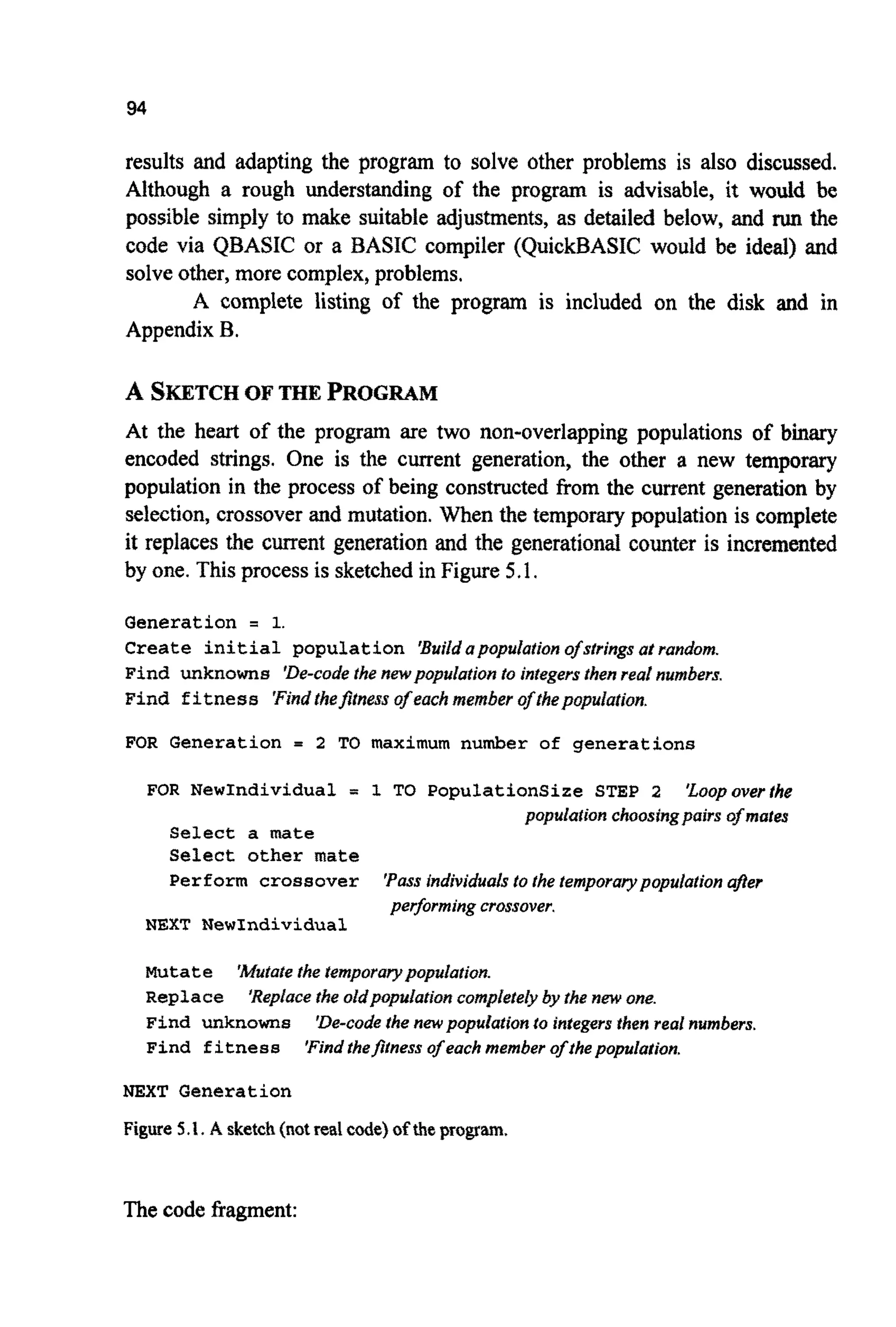
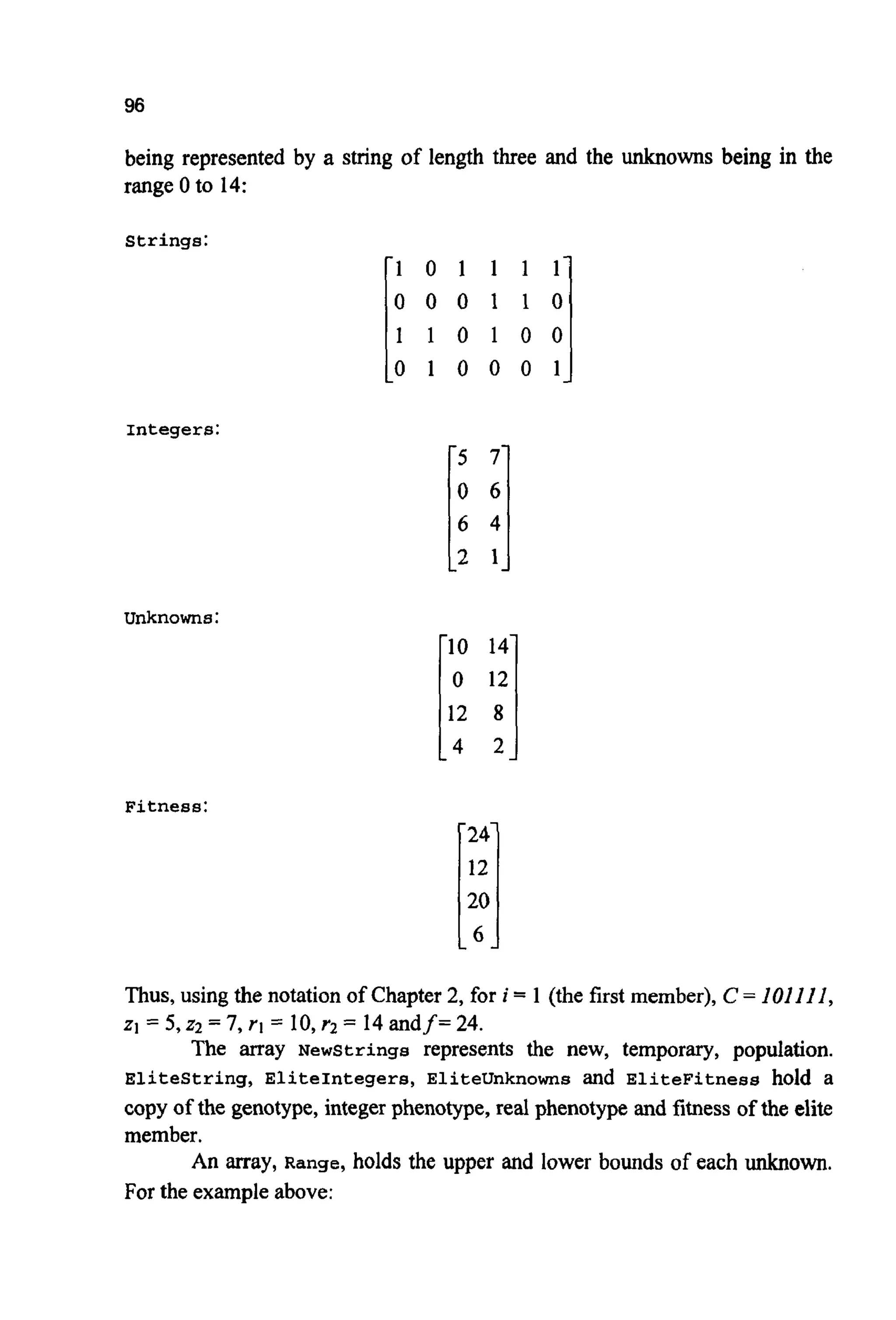
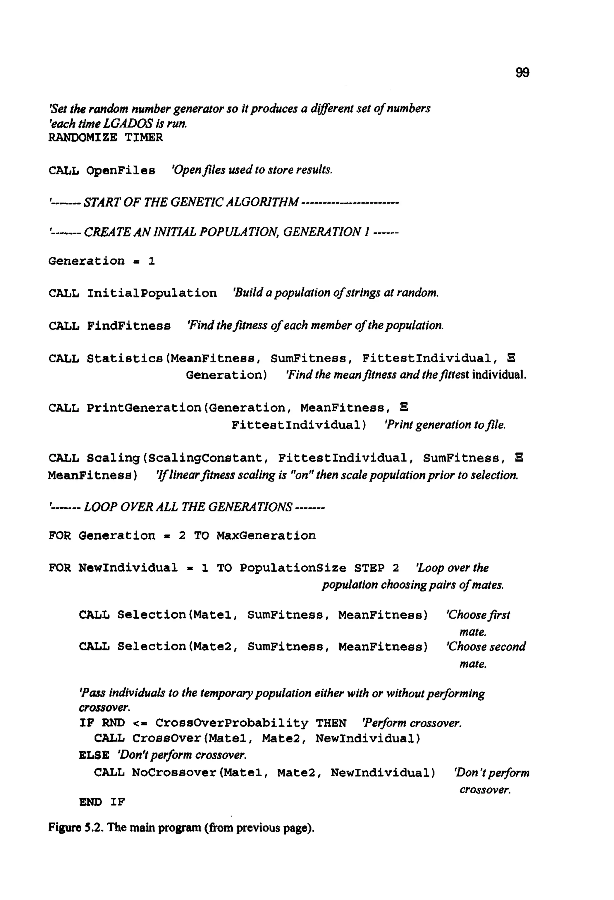
130. 113
CHAPTER6
APPLICATIONSOF GENETICALGORITHMS
A quick search of a publication database shows that the number of GA
applications is growing on a daily basis (Figure6.0.1). The range of
applications is truly stunning, including evolving computer programs
[K092,K094],estimations of protein structure [SC92]and designing water
networks [HA97].
The eight applications given in this book have been chosen for several
reasons: they are allpractical applications in scienceor engineering; all except
one uses relatively simple binary-encoded GAS of the type described in the
earlier chapters; further, they complement rather than echo the applications
given in other texts (discussed below). Although the requirement that the
examples use only binary representations and no techniques not covered in the
earlier parts of the text has somewhat limited the range of applications that
could be presented, this has been done to forcefully demonstrate that relatively
simple algorithms can help in solving complex problems. Each application
attempts to illustrate some of the difficulties in applying GASto various real-
world problem domains (Table 6.0.1). They range from the simple estimation
from experimentaldata of five real-valuedunknowns, to the use of a messy GA
to solve a complex water network problem.

131. 114
I 1 I I
1990 1992 I994 1996 I
Year
‘8
Figure 6.0.1. The continuing growth in the number of papers using GASpublished each yeru
indicates a burgeoningacceptanceof the technique. (Data obtained by searching for the string
“geneticalgorithm”within the scientificpublicationsdatabaseat the Universityof Bath;papers
within other fields are thereforenot included.)
I Applicatjon
6.1 image Registration
6.2 A SimpleApplication: Recursive
Predictionof Natural Light Levels
Main attributes
use of a simpleGA (LGA);
at most 25 real-valuedunknowns;
use of an approximatefitness function
which growsin accuracywith time.
GA applied ina recursivemannerto a
fitness landscapethat is not static, i.e. the
algorithm is hunting a noisy moving target
and two identical,but time separated,
genotypesmay not giverise to identical
valuesof fitness;
a simpleleast-squaresproblem comparing
an experimentaldata set with a simple
model;
few unknowns and limitedaccuracy
required;and
(therefore)a shortstring length.

132. 6.3
6.4
6.5
6.6
§ Apnlication
WaterNetworkDesign
Ground-StateEnergy of the fJ Spin
Glass
E s t ~ t i o nof the OpticalParameters
ofLiquidCrystals
Designof EnergyEfficientBuildings
115
Main attributes
b
b
b
b
b
b
b
b
b
b
b
b
b
b
b
discreteunknowns;
Graycoding;
linearrank selection;
uniform crossover;
a penalty functionto handle unfeasible
solutions;and
therequirementfor only a ne~-optimal,
but robust, solution.
long genotypes,L 3000;
largenumber of Booleanunknowns, M >
3000;
inclusionof anadditionallocalsearch
heuristic(directed~utation);and
directco~es~ndencebetween the
problem-space andthe string
representation,negatingthe need to
encodethe unknowns.
the developmentof a systemto replacea
previouslyhuman-guided searck
use of a seriesof sequentialadaptstionsto
a simpleGA;and
the inclusion of a traditionalsearchroutine
to create a hybrid algorithm.
a range of differentvariabletypes(binaty,
integer and real);
the need for a diverserangeof
approximatesolutionstogether with the
globaloptimum;
the need for h u ~ a n - b ~ e dfinalselection;
and
the need to avoid re-estimatingthe fitness
of any alreadyprocesseddesign.
use of remainderstochasticsamplingand
a generation gap

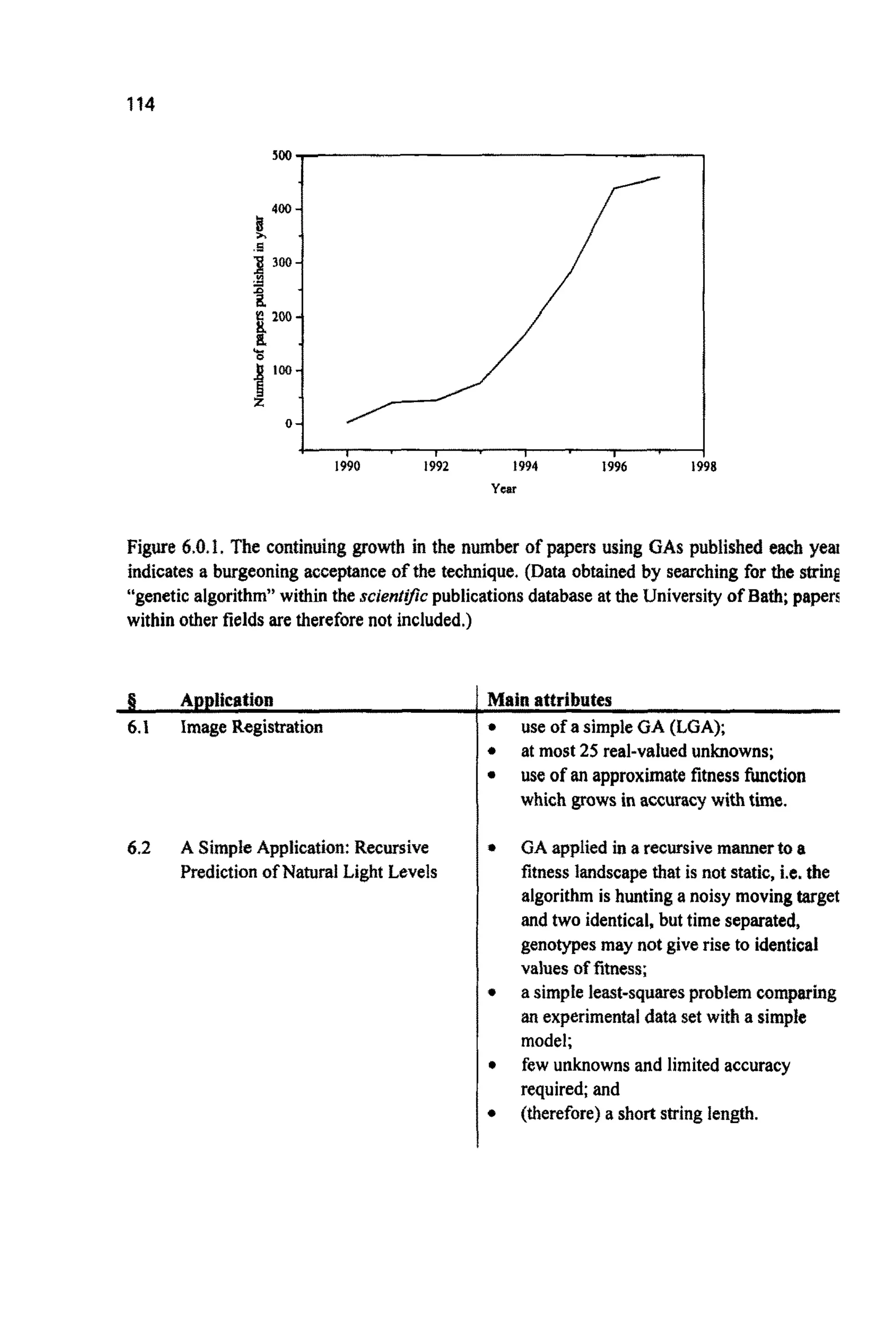
133. 116
4 Application
6.7 Human Judgement as the Fitness
Function
Main attributes
a GA being driven by aestheticjudgement,
rather than a numerical measure of fitness,
a problem where identical genotypes may
be given non-identical values of fitness;
and
a system where relatively few fitness
evaluations are possible.
6.8 Multi-objective Network
Rehabilitation by Messy GA
a sparse problem space;
use of a messy algorithm;
a multi-objective problem; and
fitness sharing.
Table 6.0.1 the various problems detailed in this chapter and their main attributes.
As with any book, the number of applications is limited by spatial
constraints. If none of them match your own areas of interest, the following
introductory texts should be studied for further applications and references.
Alternatively,an electronicsearch should be made of a publication database.
Davis [DA91]
Parametric design of aircraft
Routing in communicationsnetworks
Robot trajectories
Nonlinear systemsand models of internationalsecurity
Strategy acquisition
Artificial neural networks
Mineral separationby air-injectedhydrocyclone
Fault diagnosis
Conformationalanalysis of DNA
Interpretationof sonar signals
Engineeringdesign
Travelling salesmanproblem
Scheduling
Goldberg [GO891
Optimisationof engineeringstructures
Iterated prisoner’s dilemma

134. 117
0 Machine learning
Michalewicz [MI941
0 The transportationproblem
0 Travelling salesmanproblem
0 Graph drawing
0 Scheduling
0 Partitioning
0 Robotic path planning
0 Machine learning
Mitchell [MI951
0 Evolving computer programs in LISP
0 Cellular automata
0 Time series analysis
0 Protein structure
0 Evolving weights, learning rules and architectures for artificial neural
networks
0 Use of GAS in modelling evolution, learning, sexual selection and
ecosystems.
Zalzala and Fleming [ZA97]
0 Control systems
0 GASand fuzzy logic
0 Artificial neural networks
0 Chaotic system identification
0 Job shop scheduling
0 Robotic systems
0 Aerodynamics
0 VLSIlayout
6.1 IMAGEREGISTRATION
Genetic algorithms have a long history of use in image registration and in
particular with medical image registration [for example FI841. This is not
surprising as one can easily imagine that many such problems will contain
search spaces littered with local minima. Unlike x-rays, modern medical
imaging techniques also have the distinction of generating three-dimensional

135. 118
visualisations of the human body, greatly increasing the scale of the search
space.
The work reported here is taken from work by Coley and Bunting
[CO94] and Wanschura, Coley, Vennart and Gandy, and attempts to register a
pair of time-separated magnetic resonance imaging (MRI) data sets. (This time
separation may be over several months and with the images recorded on
differing machines.) The technique is useful for monitoring small changes in
anatomy, such as disease progressionwith time (e.g. degradation of cartilage in
arthritic disease), pre/post-surgical studies and signal intensity (e.g. functional
brain imaging) in otherwise identical images. It provides a simple application
of a GA to a problem requiring:
0 the use of a simple GA (LGA);
0 at most 25 real-valued unknowns; and
0 (because of the large amount of experimental data) the use of an
approximate fitness function which grows in accuracy with generation.
INTRODUCTION
Even when taken with registration in mind, time separated MRI data sets are
unlikely to be perfectly registered. Misalignment of the object under
investigation within the RF coil, small anatomical changes and changes in
system settings will all affect the registration of the images. This misalignment
is unlikely to be of concern if the images are presented as planar slices through
the objects and the time-separated sets are kept distinct. However, if an
accurate determination of very small changes is required, the images will
require to be registered before further operations (e.g. subtraction) are
performed. The approach adopted for identifying changes by registration is
based simply on a calculation of pixel by pixel intensity difference followed by
subtraction.
To obtain the registration the first image must be transformed
(translated, rotated or deformed) until the best match with the second image is
found. The similarity of the two images can then be quantified in a cost
function, Q. By using a numerical optimisation method to find the minimal cost
(or maximal similarity) a fully automatic procedure to extract the region of
interest is produced.
MRI data sets typically contain in excess of 16,000points per image,
and the search space for implementing registration is likely to contain a large
number of local optima which do not give the correct alignment of the images.
Although the GA has been promoted as an aid to the registration of medical

136. 119
images taken by different techniques (e.g. MRI together with X-ray)
[FI84,HI94,NI96], little work has been carried out to indicate the accuracy of
the method when used on typical pairs of time- pa rated MRI data sets
[CO94,CO96], In particular, the abilitiesof the method have not been studied
for sets misregisteredby amountstypical of clinical scans. (The data sets used
in this study were collected for other general purposes, and not with
registsationin mind).
METHOD
The two image data sets were stored as greyscale (0-255) intensities of
128x 128 pixels. Automatic registration of the two images requires (a) a
~ s f o ~ ~ t i o nand (b) a measure of s j r n ~ ~ ~ ~ .The transfo~ationapplied is
givenby the following:
X =a,+a,x+a,y +tgz+a,xy +a,xz +a,yz -!-u+yz, (6.1.1a)
5i=a,+agx +q,z+aI2xy+ +a,,yz +qsxyz (6.1.1b)
and
Z=at6+a17x+a18y+a19z+a20xy+a,,xz+a,zy~+a,,xyz, (6.1.lc)
where x, yt z are the three Cartesian spatial dimensions and the at are the
adjustableparameterswhosevalues we are trying to estimate (z = E = 0in the
2-Dw e , leaving eight ~ 0 ~ s ~ .The ~ ~ f o ~ a t ~ o ncan be v ~ s ~ ~ s ~as a
rubber cube which allows the image to be translated, re-scaled, sheared or
rotated. For example,ao, ag and a16 describethe translationof the image in the
x-, y- andz-directionsrespectively.
Themeasure of fitness, or successof the transformationis based simply
the ~ i n t - b y - ~ i n tabsolutedifferencebetweenthe two images:
(6.1.2)
where m =number of points considered, Ac = colour (or greyscale intensity)
difference between the same point in the first and the transformed second
image, and A is a constant to convert the minimisation to a maximisation,
(Morecomplexmeasureshave been suggested[T077,BR91].) Becausethe two
images may well have differentoverall intensity dis~butions(due to the way

137. 120
the imaging machines were staffed and operated-with the time separation
possibly being over several mon~s)an additional~o~ parameter, ff24, is
required to equalised the distributions:
where ciu) and c20) are the individual colours (or greyscale intensi~ies~of
pixeljfor the two images. (Note,9 4 is the same for allj.)
APPROXIMATEFITNESSESTI~ATION
To speed calculation, the pointsj must be kept to a minimum. Initial
filtering is carried out by excluding all points with near zero intensities.Most
of these points represent the backgro~dblack outsidethe anatomic^ structure
being studied.This typicallyhalves the number of points processed. Pixelsj are
selected as a random subset of the complete data (this subset must be large
enoughto contain a statisticalrepresentationof the image, initially2-3%), with
the size of this subset growing as convergence is reached [FI84]. It is this
statistical approach which is responsible for much of the efficacy of the
approach. Because of the high levels of noise within the images, much of the
intensity of a pixel within this subset might simply be stochastic in nature. To
alleviatethis, the intensitiesof pixelswithin the imageswere averaged with the
surroundingones. For g= 1, and 2-D images, this smoothing took place over
25 pixels centred on the pixel in question, the size of the grid reducing to unity
byg=G.
LGA was used with N = 50 initial guesses, Pc= 0.8 and Pm=0.001.
The registration obtained by the method can be demonstrated by comparing
slices fiom subtractions of the two sets, with and without a transfo~~tion
being applied.
In order to test the accuracy of the approach outlined above, the
technique was initiallyapplied to the problemof registeringtwo time-separated
images (Figure6.1.la, average pixel intensity, Z,=49.8, <r = 45.9 and
Figure6.1.lb, lm = 53.4, (z =50.3) of the right-hand index distal-
interphalangeal(DIP)joint of a healthy volunteer.
3-D images with 200pm in-plane resolution were collected with 16
contiguo~sslices of 1 mm thickness. After the initial scan, the frnger was
removed from the RF coil, then repositioned within the coil ready for the
second imaging experiment. (This repositioning mechanism has been found to
be inherently inaccurate, and can often result in m i s a l i ~ e n tof the joint by
the order of mm.) A secondset of images was taken, and upon completion, the

138. 121
central image slice from each data set was selected, and the GA applied to
align the two sets.
Figure 6.1.1. (a) Planar slice through image set 1: distal-interphalangeal joint in sagittal
section. @)Equivalent planar slice through image set 2. Note, the finger is displaced by
approximately2 mm. (The figuresarebinary versionsof the 256 grey-scaleintensitiesused.)
RESULTS
The generation, or time, evolution of the fitness is displayed in Figure 6.1.2.
The solution is seen to have converged after approximately thirty generations.
This point took approximately 20 s to reach on a personal computer,
demonstrating the efflciency of the algorithm-which was implemented in
PASCAL.

139. 122
0.575
0.920
0.915
'I
0.910
0.903
0 . 9 0 '
-
.., - - - -
-
-
- ;
- ;
' ' 1 " " " ' 1 "
Figure 6.1.2. The time evolution of the fitness; the highest fitness within any generation is
shown as a solid line, the mean fitness of the population as a dashed line.
The degree of misalignment reduction can be viewed by comparing
subtractionsof the data sets with, and without, the transformation. Subtractions
of correctly registered, identical, sets should result in totally blank images.
Subtracting the two images given in Figure 6.1.1, without first applying a
transformation, results in Figure 6.1.3a (Im = 25.4, (T = 30.9). The "ghost"
image seen is typical of misalignment. The only enhancement to the final
image is noise reduction by rejection of very low intensity pixels. For
comparisonan image obtained by identical subtraction,but after applicationof
the transformation generated by the GA, is given in Figure 6.1.3b (I, =2.1, (T
= 11.1). The ability of the GA to accurately align the images is clearly shown
by there being almost no structures in the image, and no ghost image (also
implying that there are no anatomical differences between the two data sets);
what remains is essentially noise. A more quantitative measure of alignment,
apart from the much reduced values of I,, and (T, is the number of fully
connected pixels, PJ,which reflects the information content of the image. A
pixel is fully connected if, and only if, it has a non-zero intensity and its eight
nearest neighbours also have non-zero intensities.If the two images have been
successfully aligned to the image resolution (1 pixel, or 200pm) then
subtraction will give Pf=O. For Figure 6.1.la and 6.1.lb, Pf= 15793 and

140. 123
15723 respectively; for Figure6.1.3a Pf= 12907, and for Figure 6.1.3b, Pf=0
indicatingregistration.
The technique is useful for monitoring small changes in anatomy, such
as disease progression with time (e.g. degradation of cartilage in arthritic
disease), pre/post-surgical studies and signal intensity (e.g. functional brain
imaging)in otherwise identicalimages.
Figure 6.1.3a: Planar slice after the subtraction of the images without the GA-based
registration. The ghost image of thejoint is due to misalignment of the data sets. Figure 6.1.3b:
Planar slice through the subtraction of the images after the GA-based registration; almost all
misalignmenthas been removed. (Note, these figures are binary versions of the 256 grey-scale
intensitiesused.)
6.2 RJECURSIVEPREDICTIONOF NATURALLIGHTLEVELS
Controlling artificial lights within buildings to act solely as a supplement to
available daylightingrequires continuous knowledge of natural lighting levels
within each room. Although this information is readily obtained by
measurementwhilst lightsare extinguished,once illuminatedthe determination
of the underlying natural light level is not so straightforward.This application
describesthe use of a genetic algorithm as the heart of a self-commissioning,
adaptive algorithm capable of the real-time prediction of natural light levels at
chosen points within a room using external measurements of vertical and
horizontal plane illuminance. Such a system forms the basis of a robust and
practical lightingcontroller.

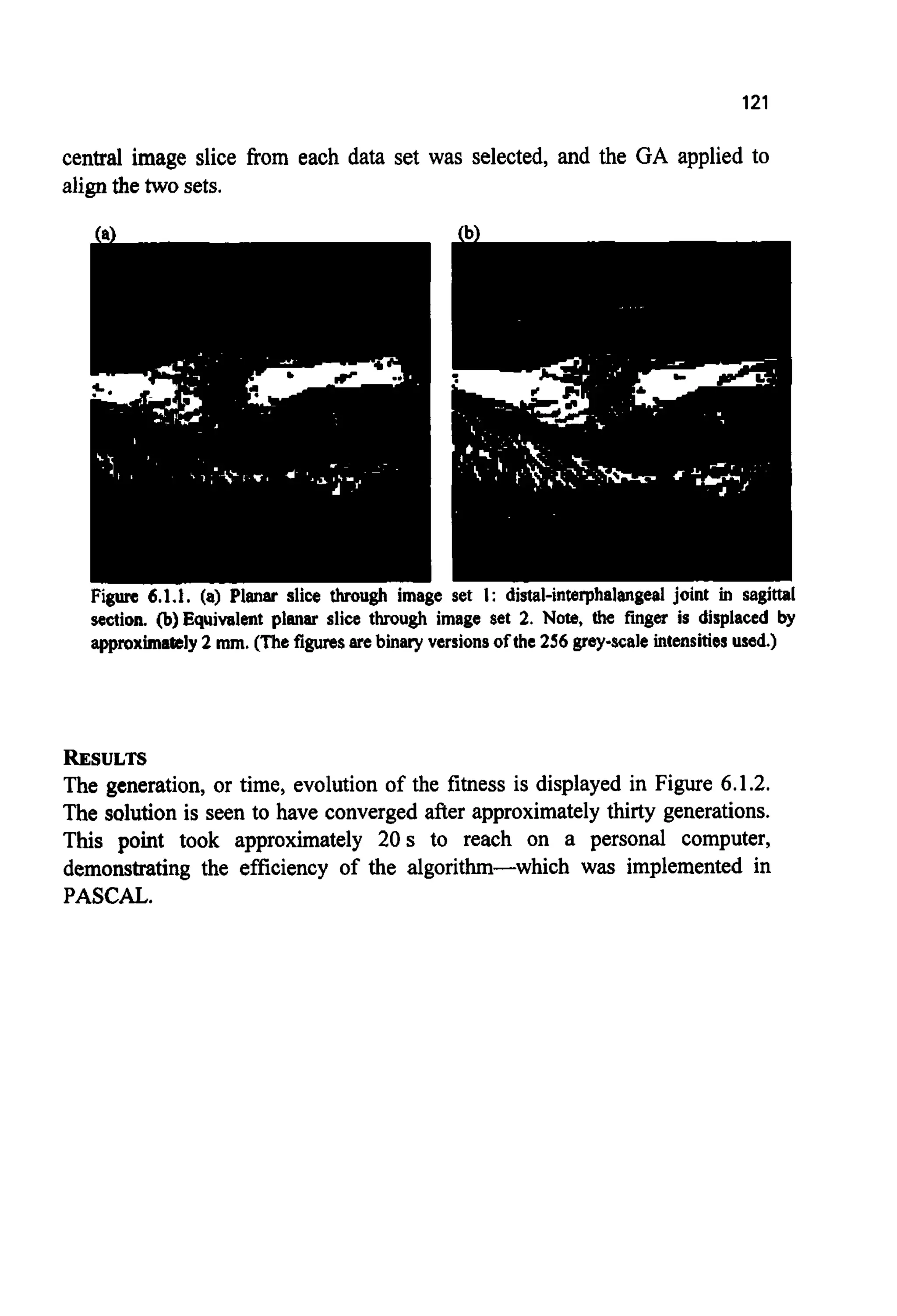
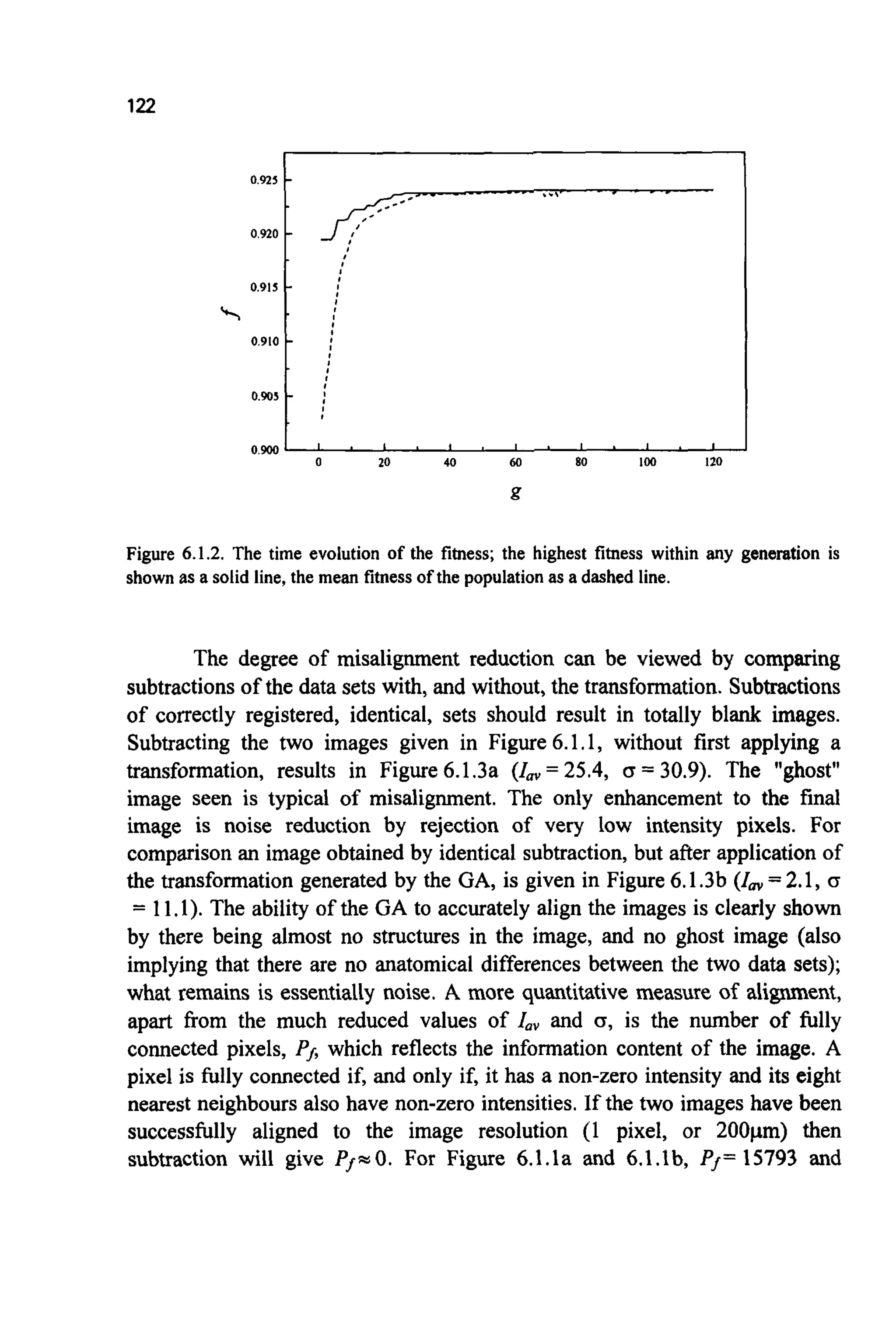
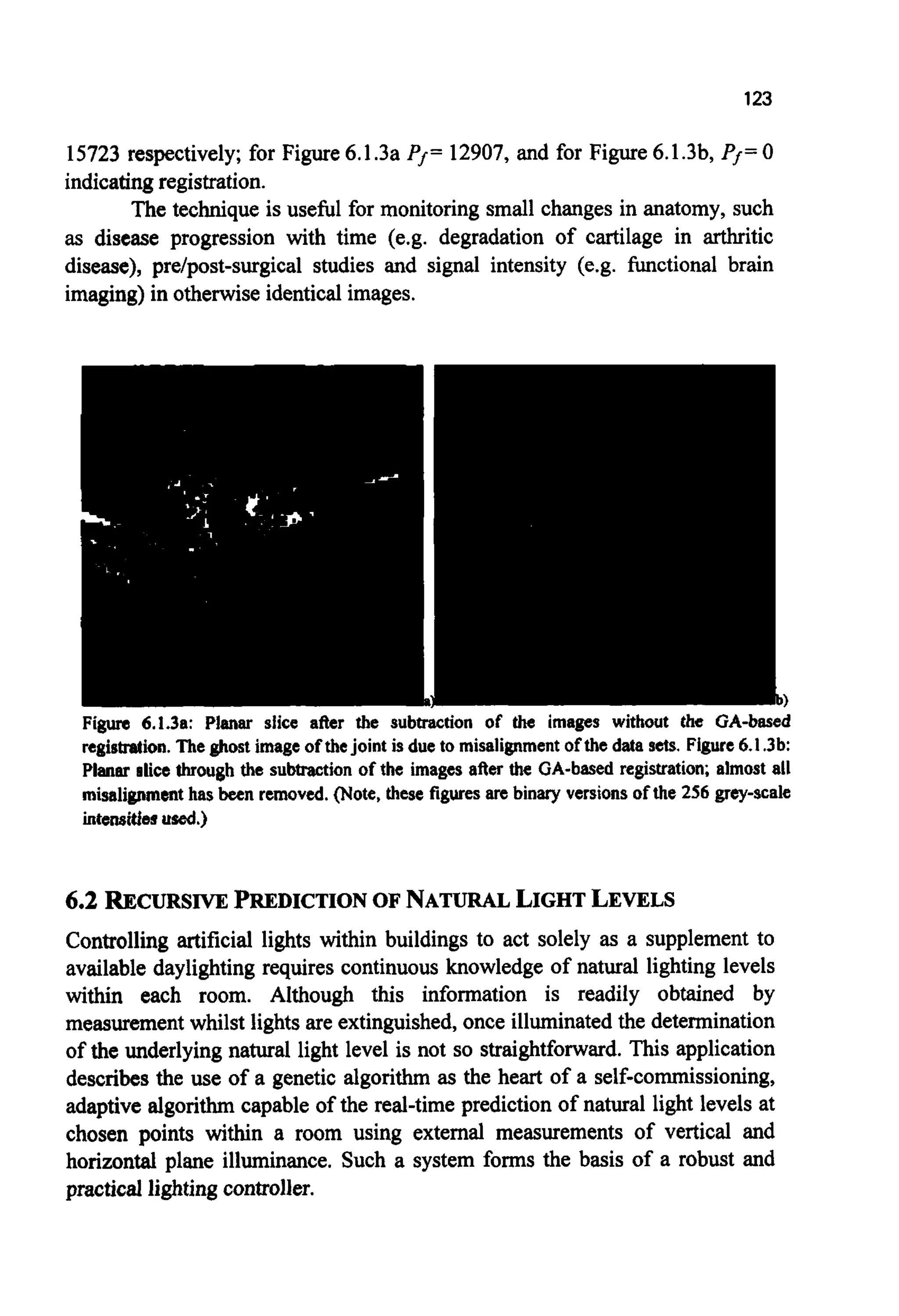
141. 124
This application(based on reference [CO97]) is very simple, requiringonly
the identificationof five unknowns-the accuracy of which is not particularly
important.The GA is applied in a recursive manner: as new sets of data arrive
the algorithm is re-run, without re-initialisation, for a fixed number of
generations.The results are compared with those found by a traditionalmethod
[C094a]. It illustratesthe following:
a binary coded GA applied in a recursivemanner to a fitness landscapethat
is not static, i.e. the algorithm is hunting a moving target and two identical,
but time-separated, genotypes may not give rise to identical values of
fitness;
fitness-propo~ionalselection;
singlepoint crossover;
a simple least-squares problem comparing an experimental data set with a
simplemodel;
a search space knownto contain local optima;
many equallypossible,often distant,solutions;
few generationsto convergence;
few unknowns;
limited accuracyrequired; and
(therefore)a short string length.
I N T ~ O D U ~ I O N
This application discusses the employment of a GA to the problem of
predictingthe natural horizontalplane iliuminance(i.e. that falling on a desk or
worksurface) within a room, ftom measurements of illuminance outside the
building envelope and at some point distant. Attempts at such predictionshave
been made before [C094a] using a recursive least squares algorithm, allowing
results for a GA to be contrasted with those of a traditionalalgorithm.
Lighting is often the largest single item of energy cost in offices and
considerablesavings can be made [EEOI] implying reductions in both cost and
resultant emissions of gases implicated in global warming, Savings can be
effected by a com~inationof higher eaciency lamps, more efficient fittings,
better controls and increasedusage of da~~~ghting.Here the approachis anovel
lighting controller which enables maximum use to be made of available
daylight.
The availability of high levels of natural light within a space is not, of
itself, sufficient to ensure that less use will be made of artificial lighting. For
manually controlled systems, studies have shown [HU79] that it is the

142. 125
perceived level of light on initially entering the room which chiefly determines
whether lights will be illuminated. Once switched on, it is very unlikely that
they will be switched off-notwithstanding any subsequent increase in natural
light levels. Automatic photocell-based controllersface a similar difficulty. It is
straightforward for such systems to prevent the initial use of artificial lights if
levels of natural light measured at internal sensors are high enough to obviate
their use. Once illuminated, however, it is more difficult to decide whether the
underlying level of daylighting is sufficient to enable them to be extinguished.
There are various solutionsto this problem.
One apparently attractive approach to the problem is to make
measurementsof external lighting levels and to relate these to expected internal
levels. This is far from easy to accomplish. The relationship between internal
and external illuminance is time-dependent on an hourly and seasonal scale.
Thus any attempt to determine a simple ratio which relates the two is unlikely
to be successful. A better approach would be to relate external horizontal and
vertical plane illuminance, in a number of directions, to internal horizontal
plane illuminance [HA88]. The advantage is that vertical plane illuminances
contain directional, and therefore time, information. A means must still be
found, however, to determinethe ratios which relate the various componentsof
vertical plane illuminance to internal conditions. This can be done by
calculation for each space, but there is a better approach, which also allows
such ratios to be time-dependent.
Experience with lumped-parameter thermal models [CR87,CR87a] led
to the development of a computer routine for the real-time identification of the
model parameters from the measured building response to energy inputs
[PE90,PE90a,C092]. There is obvious potential here for application to the
lighting problem just discussed. Given a simple model relating internal
horizontal plane illuminance to the separate components of the external
horizontal and vertical plane illuminance, a similar technique could be used to
identify the unknown parameters as employed in the thermal case. Such an
approach was successfully tried [CO94a] by using a recursive least squares
algorithm. However, although the average error was found to be small, the
largest errors in prediction (which were possibly systematic) occurred during
times of high illuminance, just when any practical controller should be
signalling for the artificial light to be extinguished.It was unclear whether this
poor performance was due to the model or the algorithm used. It was decided
to see if better predictions could be made by using a GA, thus hopefully
lending support to the model. If indeed the GA did perform better, this would

143. 126
probably imply it had successfullynavigated around one or more local optima
to a better solution.
THEMODEL
The model chosen to relate the internal horizontal plane illuminance I$, at
time t, at a given point in any room m in the building, to the five external
measured vertical and horizontal plane illuminances,4"",falling on the roof of
the building, was the simpleparameterisation,
(6.2.1)
where the bi are the numerical attenuation coefficients which contain
information on, for example, the atten~tingpower of the windows and the
reflectivityof internaland externalsurfaces.
It is worth noting that the model described here does not need any
information on the alignment of the external sensors, nor does it require
knowledgeof the orientationof the windows. This will allow any systemthat is
developedfrom this model to be largely self-co~ission~ng.
Equation (6.2.1) is a somewhat arbitrary par~ete~sationof the
problem. Thus the Hrnwill not, in general, form a linearly independent set.
However this should not be a problem as there is little need to find a unique set
{b}, but only any set in the parametric space which is capable of representing
the response of the system. This will only hold true if no attempt is made to
place a precise, physical meaningon the individu~elements of {bf,but instead
to regard them solely as parameters. It is known [CO94a] that the space
contains many local optima and that there are many sets {b} able to provide
solutionsof variousaccuracy.
PARAMETEREXTRACTION
For any particular room, (6.2.1)is of the form
5
x, = C a j x , .
J'1
(6.2.2)
E q ~ t i o n(6.2.2) is the form needed for the classical linear least-squares
problem in which a set of unknown parameters { a ) describing an observed

144. 127
system is to be determined from k measurements at differenttimes of a set of
observables{ x }.
In the linear least-squares problem it is assumed that the k successive
measurementsof the setx can be representedby
N
x,, =Cajxj,+E, .
j-1
(6.2.3)
where i = 1,2 ...k; siis an errorterm, and in this caseN = 5.
Although strictly speaking the €j should be Gaussian and serially
uncorrelated, least-squares gives reasonable results with most error
distributionsencountered in practice. Specifically,estimatesdj of the unknown
parametersuj are chosento minimisethe functionsd, where
(6.2.4)
In order to solve (6.2.4) using a GA, the five unknown parameters
represented by the elements of { Ci } were encoded as binary strings of length
10. Using the knowledge gained from reference [CO94a] it was decided to
limit the search range to f100. Thus the search space is discretised to an
accuracyof better than one part in a thousand.
SECULARTRENDS
In (6.2.4) the sum runs over all values of i, i.e. all the collected data. This has
the advantage of smoothing fluctuationsin the data caused by inaccuracies in
the measurements (caused, for example,by the temporary use of blackouts, or
wildlife interfering with the external sensor), thereby stabilising the values
stored in { Ci }, and making the algorithm robust. However, although stability
against fluctuationsin the data is a good thing, there is a desire to track secular
trendsin the response characteristicsof the system:for example,the dirtyingof
windows or the constructionof a nearby building. This problem can be solved
by various methods [YO74]:for example, by using an exponentially weighted
past averaging method to curtail the memory of the estimation procedure in
least-squares analysis. In systems where the variation of the parameters is
knownapriori, more advanced methods can be used, for example the Kalman
filterestimator [KA60].As very little upriori information of the nature of the
time variation of the parameters has been assumed, a simpler method is

145. 128
adopted. The sum in (6.2.4) is run over a sliding window of fixed width w.
Thus the arrival of a new data point (the p )causes the sum to run from k-w to
k.
As any trends are presumed to be slow, consecutive predictions of { ir }
are likely to be similar. Thus it would seem appropriatenot to the reset the GA
to a random initial population upon receipt of a new data point. The initial
population is simply set to the final population from the last run.
APPLICATION
A computer code ILLUMIN was written to apply LGA to the model and
calculatethe five unknown parameters that characterisethe responseof a room.
The data analysed here were recorded at the Physics building of the
University of Exeter during the spring of 1992. Five light-sensitive resistors
were attached to the top and the four vertical faces of a small plastic cube. This
sensor array was housed in a glass enclosure and placed on the roof of the
building. Within a room in the same building a single sensor was set in a
horizontal orientation to measure the internal light level. The time series of
measurements from these sensors was monitored constantly and recorded on a
data logger every ten minutes (Figure 6.2.1). Two consecutive sets were
collected, one for training of the GA and the other for testing the results.
0 25 50 75
Data Points i (recorded at 10 min. intervals)
Figure 6.2.1.A short fraction of the time series of measurements from the five external sensors
(nocturnal periods removed),with each line representing a different sensor.

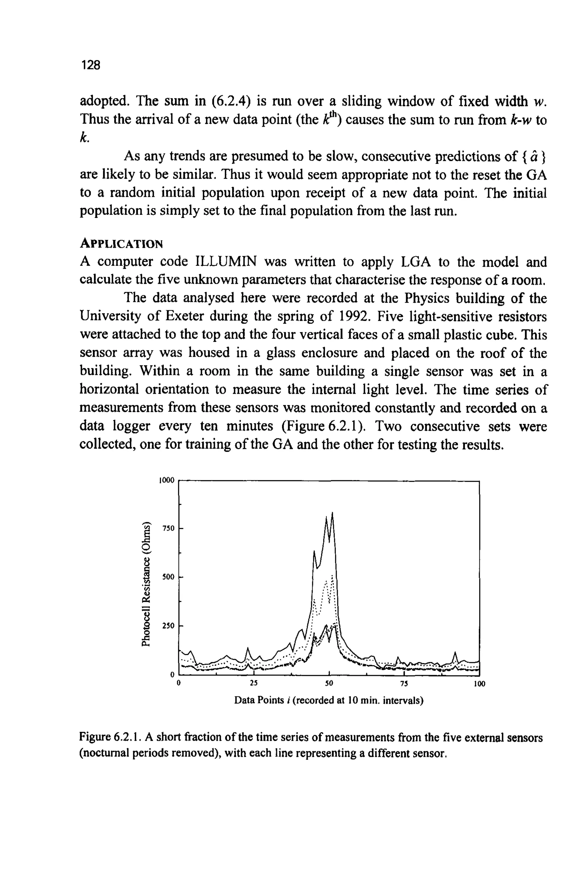
146. 129
RESULTS
Table 6.2.1 showsthe parameter values identified by ILLUMM using the first
seven days‘ data, together with the values found by the recursive method.fr
was foundafter24 g e n e ~ t i o ~forN = 100,P, = 0.005, P,=0.6,E = I,fitness-
p r o ~ ~ o n ~selection, and w set to the width of the data set. The mini~sation
of (6.2.4) was recast as a m~imisationof fitness by settingf=A -Q, where
the constantA is large enough to ensurefis positive. The identified values are
similar, but not identical,to those produced by the traditional recursive method
[PLSO].
12.156
0.5328
22.522 21.9
22.262 22. 1
-36.713 -35.8
Table 6.2.1. Ttte fmal (dimensionless) parameter values found by recursive least squares
[CO94a]andbythe geneticalgorithm,forthe dataof Figure 6.2.1.
The model represented by (6.2.2) and the fit represented by the
parametervalues given in Table 6.2.1can be tested by using (6.2.2)to generate
a time series of internal light levels, and comparing this with the second
observed series (Figure 6.2.2). The results from the GA show exceptionally
good agreement and a large improvement (particularly at higher light leveb)
over those fkom the classical recursive least-squares algorithm. The final
parameter set is found to predict the internal light level from observed external
levels to within an RMS error of 3% at an i l ~ ~ i n ~ c eof 500 lux. This
improvementimpliesthat the GA has better navigational propertieswithin the
space. In particular, as both solutionsare close, not just in terms of the result
but the parameter set itself, it would seemthat the GA was ableto “jump” over
one or more local optima to find a better solution. However, without an
enumerative search of the space it is impossible to say if the values found
represent thetrue global optimum.
In practice k extends indefinitely, and thus many totally separated sets
of widthw are collected so that the controller can take account of slow secular
trends in the parameters (caused, for example, by seasonal transients in the
reflectivity of the land s ~ o ~ d j n gthe building and changes in tree foliage).
This adaptive mode is also suitable for sign~lingexcursions in the fitted

147. 130
attenuation parameters beyond pre-determined limits (caused, for example by
the failure of the occupants to open curtains). The method has proved
successful with w = 600 and the GA being re-run without re-initialisationfor a
further 24 generations for each subsequent set. An alternative approach might
be to set w = 1 and only allow the algorithm to advance a single generation for
each new data point. However, because of the possibilities of large errors in
individual data points, due in this instance to environmental factors, the
performance of the GA might well be compromised.
This opens the way to integrating such models with lighting controllers.
Such a controller would employ this technique to maintain an updated estimate
of the attenuation factors, {b}, during periods when artificial lights were not in
use. Once the lights were illuminated, the controller would use the model
represented by (6.2.1) to predict natural internal light levels from the
continuing measurements of external light levels f:. If the predicted internal
illuminance exceeded a predetermined threshold value (set by the occupants),
the controller could then call for the artificial lights to be extinguished. Such a
prototype has been used to control the illuminationwithin an office space,
-2000 " ' " " " " " ~
0 100 ZOO 300 400 JW 600 700
Data Points i (recordedat 10 min.intervals)
Figure 6.2.2.Comparisonof measured and predicted light levels (nocturnal periods removed):
GA solid line, recursive classical dotted line, and measured dashed line.

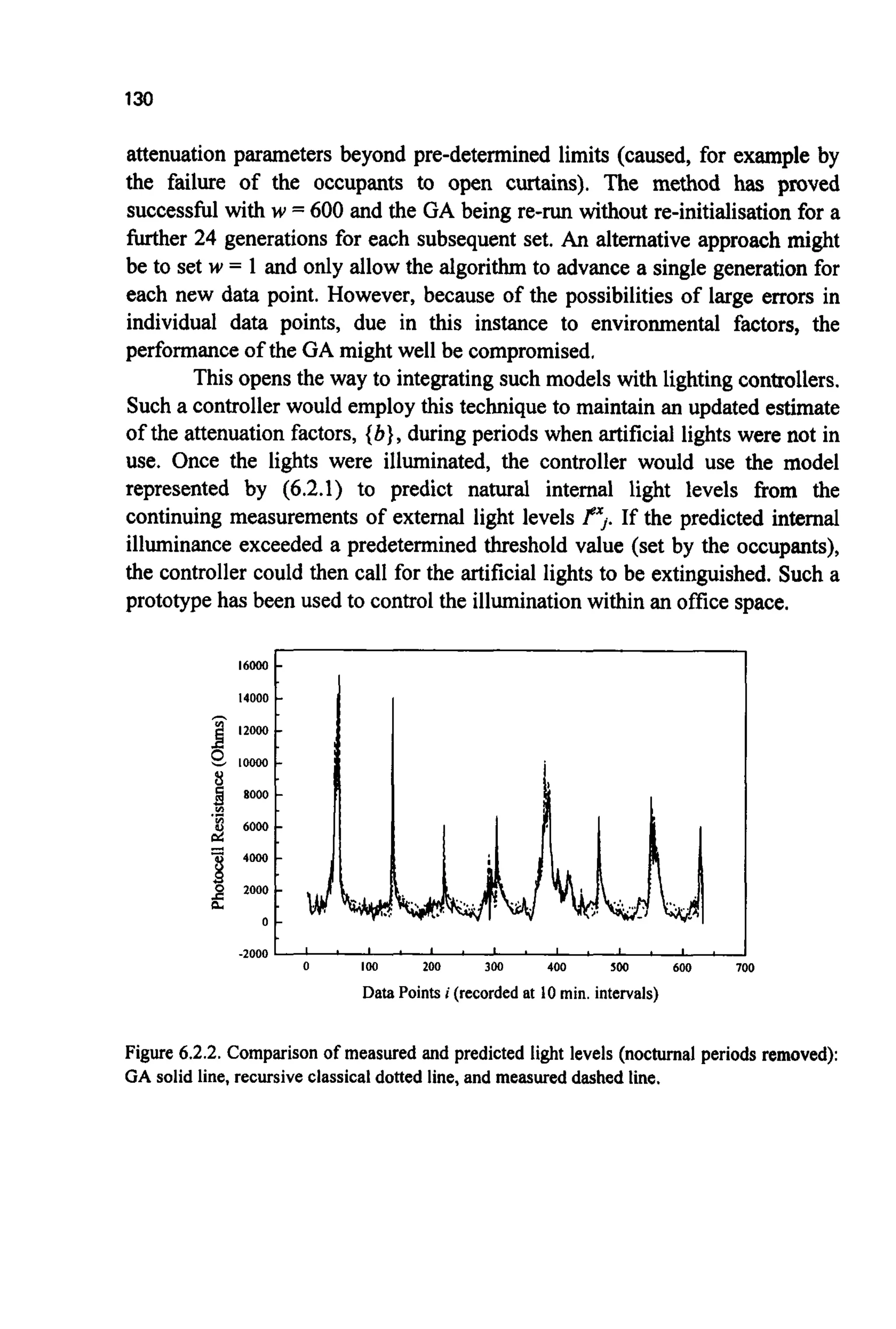
148. 131
6.3 WATERNETWORKDESIGN
Such is the scale of infrastructural asset represented by a large water
distribution networkthat the use of a sub-optimaldesign can have considerable
cost implications. Unfortunately the complexity of such systems is such that
the identification of the optimal design for a particular network is far from
easy. By developing a GA-based design tool, GANET [SA97], for water
distribution network planning and management, Godfrey Walters and Dragan
Savicare attemptingto rapidly identify near-optimalsolutions.
In the work described here [SA97], GANET was applied to both
illustrativeand real water networks. The following features are exhibited:
0 discrete unknowns;
0 Graycoding;
0 linear rank selection;
0 uniform crossover;
0 a penalty function to handle unfeasiblesolutions;and
0 the requirement for only a near-optimal,but robust, solution.
The penalty function is particularly interesting because it is generation-
dependent.
INTRODUCTION
The problem of selecting the optimal set of pipe diameters for a network so as
to minimise cost has been shown to be an NP-hard problemt [YA84]. The
simulation of the hydraulic behaviour of a single network itself is a difficult
task,requiring a simultaneousconsiderationof energy and continuity equations
and the head-loss function [WO93]. The actual network layout is often
determinedby such factors as the locationof roads, leavingonly pipe cost to be
minimised. The solution itself is constrained by requirements of minimum
flows and pressures at various points on the network. The pipe diameters
themselves will not in general be continuous variables, but will be defined by
the rangeof commerciallyavailable sizes.
The objective function, Q, to be minimised is the cost, c, given by a
function of pipe diameters 0,and fixed lengthsAt only:
'NP hard problems are ones that cannot be solved in polynomial-time. Essentially this means
that the complexity of the problem grows at a faster than polynomial rate as more unknowns
are added, making all but the simplest problems impossible to solve.

149. 132
(6.3.1)
where Npis the total number of pipes in the network.
Sa requires minimising under several constraints. At eachjunction node
the flow into the junction, gin, and the flow out of the junction, QOul,are
connectedthrough the continuityconstraint:
(6.3.2)
where Qe describes the demand (or inflow) at the node. For each loop within
the system energy conservationimpliesthat:
(6.3.3)
where Ep is the energy input by a pump and hf is termed the head-loss. In order
for the network to be usehl a minimum head will be required at each node.
These minim^ heads H,”” ,at each nodej form a set of constraints, H, such
that:
H,2 H,”“ ;j = 1,.....N, , (6.3.4)
where N, is the total number of nodes.
In order to confirm that any network designed by the GA satisfies these
constraints requires the solution of a hydraulic model of the system. The most
commonly used formula to describe the relationship between pressure drop,
flow rate, pipe length and pipe diameter is the empirical Hazen-Williams
(H-W) relationship [WA84]; in empiricalunits:
where v is the flow velocity, Rh is the hydraulic radius, Sf the hydraulic
gradient, and b a dimensionalcoefficient.For a pipe of length A and flow Q the
head loss is given by:

150. 133
where w is another numericalconversionconstant.
PREVIOUSSOLUTIONTECHNIQUES
It has been suggested [YA84] that only explicit enumeration or an implicit
numerationtechnique such as dynamicprogrammingcan guarantee finding the
optimal solution. The problem is non-linear due to the energy constraintsand
further ~mplicatedby the requirement to use discrete-sized pipe diameters.
The problem is NP-hard and intractable for even relatively small (Np<20)
networks. However, as is typical with many real-world problems, the inability
to guarantee an optimal solution is not of prime importance. The goal is the
identification of the lowest-cost system given a realistic amount of time in
which to do the calculation.Due to engineeringand other factorswhich cannot
be Wly described in the model, the final solution ~ p l e m e n t ~might only in
part be described by the optimum identified by the modelling processes.
Becauseof such considerationsand the limited amountof time available to find
a working solution, it is important that the algorithm identifies near-optimal
solutionsrapidly. Even if other methods are able to find better solutionsgiven
enough time, it is the p e ~ o ~ a n ~of the method within a time constraint
which is important. With a network of only 20 pipes and a set of 10 possible
pipe diametersthere are lo2' different possible designs. Clearly only a fraction
of thissearch spacecan be examinedby any practicablemethod.
Historically, much of the search space has been eliminated either by
using a simplified approach [GE85,MU92], or by additional human
i n ~ ~ e n t i o n[WA85]. Otherapproachesinclude attemptsto reduce the probIem
to a sequence of linear subproblems [SH68,FUf90].This can lead to split pipe
designs, with one or two pipe segments of differing discrete sizes between
nodes. In reality, such segmentswill need to be replaced by a single diameter
before implementation.
onl linear p r o g r ~ i n gtechniques have been applied to the problem
[EL85,DU90], but have treated pipe diameters as continuousvariables and are
limitedto problemsof small size.
Increasingly, evolutionary inspired programming methods have been
appliedto hydraulicnetworks[G087a,WA93,MU92,WA93a]
GANET: A GA MODEL FOR LEAST-COSTPIPENETWORKDESIGN
The use of a GA to solve a network problem can be illustrated by using
GANET to solve the two-loop network studied initially by Alperovits and
Shamir [AL77] (Figure 6.3.1). In the following, the GA rather than the water

151. 134
Node
1(source)
2
3
4
5
6
I
engineering aspects will be concentratedupon. In particular, considerationwill
focus upon the hunt for a near-optimal solution, the use of Gray coding, the
form of the unknowns, and the penalty function.
Demand (m’lh) Ground level (m) Minimum AcceptableHead
above ground level (m)
-1 120.0 210.00 30
100.0 150.00 30
100.o 160.00 30
120.0 155.00 30
270.0 150.00 30
330.0 165.00 30
200.0 160.00 30
Figure 6.3.1 The two-loop network used as an example (by permission of ASCE [SA97]).
The network consists of a single source with a 210m head and eight pipes
arranged in two loops. The pipes are assumed to be lkm long with Hazen-
Williams coefficients of 130.The demand and head requirements at each node
are listed in Table 6.3.1. The fourteen commercially available pipe diameters
and their cost per metre are given in Table 6.3.2.

152. 135
Diameter(In.) 1 Cost
1
2
3
4
6
8
10
12
14
16
K3
20
22
(monetary units)
2
5
8
I 1
16
23
32
50
60
90
130
170
300
Table6.3.2.Pipediameterand costdata[SA97].
VARIABLEFORM
The form of the unknowns in this type of problem is such that the mapping
described in Chapter2 between integer and reds is not required. Figure 6.3.1
showsthat there are eight decisions (the eight unknownpipe d i a m e ~ ~ ~to be
made about the network. Each one of these decisionvariables can take one of
the fourteendiscrete values listed in Table 6.3.2. The shortestbinary stringthat
can represent fourteen values is of length four. However 24= 16 not 14. This
illustrates ~ d ~ d a n c yin the coding, with two of the possible strings not
representing any available pipe diameter. The simplistic way around such
redundancy is by assigning the two additional string possibilities to other
(close) pipe diameters. This will mean that in the two cases the same diameter
is represented by more than a single sub-string, whereas the other twelve
diameters are represented by unique sub-strings. Such an approach can have
stochastic implications, although these are unlikely to be major unless the
approachistakento extremes.
GRAYCODING
The algorithmis based on a Gray binary codingof the decision variables. Such
a coding representsadjacentintegers in such a manner that they differ in only
one bit position (see Chapter4). Thus similar physical pipe diameters have
similar string representations. In many problems this adjacency property is

153. 136
more important than one might initially think. For example, if the possible
pipes in Table 6.3.2 are represented by a four-bit simple binary string, then the
followingordered list is generated:
pipe size 4-bit binary pipe diameter (in.)
representation
0000 1
0001 2
0010 3
001I 4
0101 8
0110 10
0100 6
Moving from a pipe size 3 (4 inches) to size 4 (the next size up) cannot be
achieved by flipping the value of a single bit, but requires three out of the four
bits in the string to change their value, whereas in the Gray coding shown
below, a single bit move gives a single increment in pipe size.
pipe size 4-bit Gray
0 0000
1 0001
2 0011
3 0010
4 OIIO
5 0111
6 0101
representation
pipe diameter (in.)
1
2
3
4
6
8
10
Although by using such a coding, programming the algorithm is made
slightly more difficult, the performance of the algorithm is likely to be
improved. In particular, in the later stages of a run where the solution is near
optimum and mutation is playing an important role, progression will hopefully
become faster. Another advantage is that a particularly simple bit-based hill-
climbing routine can be included as a direct search algorithm after the final
generation has been processed.
THEPENALTYFUNCTION
The objective function, 8,is particularly simple,just the sum of the cost of the
individual pipes. However, each network created must be checked against the

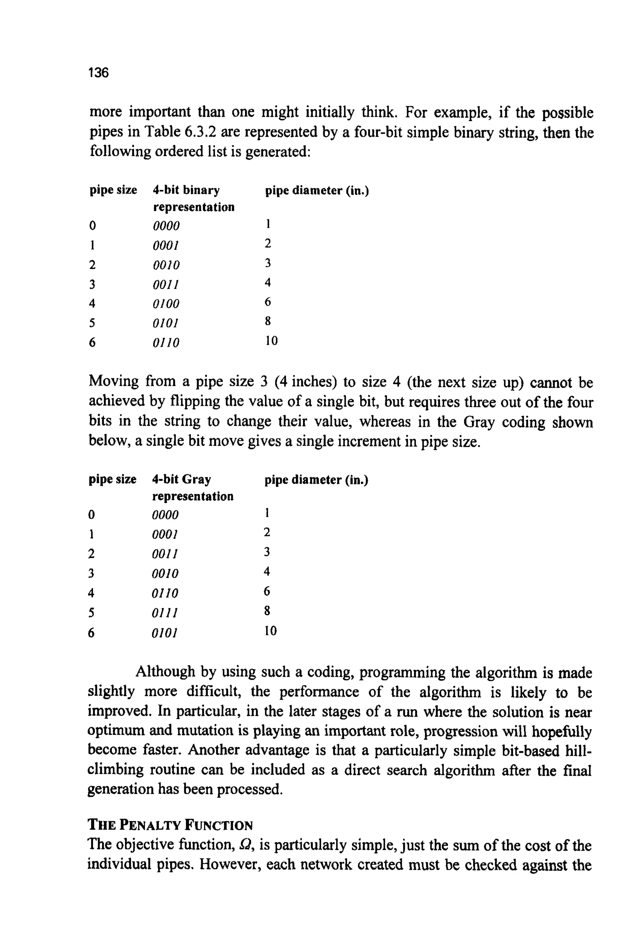
154. 137
minimumhead requirementsat the various nodes. The network solver used by
Waiters and Savicis based on the EPANET [ROS93] computer pro^. This
uses a gradientmethod [TO871for solving(6.3.2)and (6.3.3)
Unfeasible solutions, i.e. those which fail to meet (6.3.4) are not
removed from the population. Instead their fitness is degraded. If they are far
from feasible,they are likely to be viewed as "lethals"by the algorithmand fail
to reproduceat next generation.Thus (6.3.1)is replacedby,
where p is a penalty multiplier and the term in braces equals the m ~ i r n ~
violationof the pressurec o ~ ~ ~ n t .
The multiplieris chosen to norrnalisenominalvalues of penaltiesto the
same scale as the basic cost of the network. Unfeasible solutions are likely to
carrymore informationusefulto the GA earlyon in the searchthan towards the
end, when fine adjustmentsare being made to the optimal solution.In addition,
in many search spaces there are likely to be more unfeasible solutions during
the early generations. It would thereforeseem sensibleto devisea penalty term
whichbecomesincreasinglyseverewith generation.Onepossibility is:
where K is a constant. When g = G, i.e. the final generation,p should be such
that no unfeasible solution can be better than any feasible solution in the
population.
REPRODUCTION
In an attempt to avoid prematurec~nv~~genceand the need for fitness scaling,
rank selectionwas used with a linear weightingfunction.
After experimentationwith different operators, uniform crossover was
adopted.This alsoallowed(6.3.1)*which describesa minimisationproblem, to
be used directlyby simply ranking in reverse order. With P, = 1.0, P,,,was set
to 0.03, or approx~atelylIL, and elitismapplied.

155. 138
p 900-
'I
g, 800-
-9
I 700-
s
4
1 600:
'I 500-
s'
400 -
ANILLUSTRATIVEEXAMPLE
Although the network shown in Figure 6.3.1 is of modest scale, it still contains
148,or approximately 1.5x109,possible designs. This has forced all previous
studies to consider split-pipe solutions. Table 6.3.3 lists some typical results,
together with results from GANET. As different authors used differing values
for the head-loss coefficients of the Hazen-Williams formula, the results are
difficult to compare. Two GA-based solutions are presented covering the full
range of published values. The results are particularlypromising because of the
use of realistic non-split pipes and because the calculations only took
approximatelyten minutes on a personal computer.
Figure 6.3.2 shows a typical plot of the cost of the best solution as a
function of generation.The form is typical: a rapid reduction followed by much
slower progress until the termination condition (G = 500) was reached. The
best solution found was identified after approximately 130 generations. A
population size of 50 was used, implying250,000 evaluations were performed.
At most, this represents less than 0.017% of the possible pipe combinations and
therefore of the search space.
1 . 1 - 1 ' 1 ' 1 . 1 . 1 . 1
Figure6.3.2.Evolution of cost with generation(data from [SA97]).
The quality of the solutions identified, and therefore the robustness of
the method, can be gauged by hydraulic simulations of the other results
presented in Table 6.3.3. These simulations were carried out for both the
maximum and minimum values of the conversion constant w in the Hazen-

156. 139
Nods
i
2
3
4
5
6
7
Williams formulaused to produce GA results. Table 6.3.3 shows that many of
the resultsbecomeunfeasible for at least one of these bounds. This is less so of
the GA-based calculations. This indicates that the GA has identified robust
engineeringsolutionsto the problem.
Alperovitsand Goulter Kessler Eiger GA GA
Shamir et al. and et al. No.1 No. 2
[AL771 [GOU86] Shamir [EI94] a)= 10.508 o=10.903
53.80 54.15 53.09 53.09 53.09 55.86
31.89 32.78 29.59" 29.81IF 29.97IF 30.30
44.71 43.91 43.35 43.59 43.18 46.38
31.65 31.65 29.38IF 29.90" 33.13 31.61
30.83 30.83 29.69" 29.46" 30.11 30.50
31.11 31.11 29.59IF 29-34'' 30.13 30.52
[KF,89]
REALNETWORKS
GANET has been applied to the trunk network of both Hanoi [FUJ90] and
New York [SC69]. The Hanoi network consists of 32 nodes and 34 pipes
organisedin three loops,with approximately2 . 9 ~ 1 0 ~ ~possible designs.
In the case of New York the problem was one of expansion, the goal
being to identify the most economically effective designs for additions to the
pre-existing systemof tunnels.
In both cases the use of a GA provided robust solutions in a very
efficientmanner.
6.4 GROUND-STATEENERGYOF THE fJ SPIN GLASS
Spin glasses have been studied for many years by physicists as idealised
representations of the solid state. Such a representation consists of a large
number of spin sites residing on an interconnected lattice (see Figure 6.4.1).
However, interest in such systems goes beyond the world of physics and they
are currently of great interest across a wide range of fields [BI86].
Additionally, computational methods developed to study spin glasses have
been applied to questions in computer science, neurology and the theory of

157. evolution {ST89,FA94,KI87~.A well known example of this is the design of
artificialneural networks, where the Hopfield net is found to be isomo~hicto
the Ising spinmodel [R093].
One problem studied within spin glass systems is the dete~i~ationof
the ground state energy for a system of infinite size. The value dependson the
layout of the lattice, its dimension and the configuration of the bonds.
Wanschura, Migowsky and Coley [WA96] have used a genetic algorithm
together with a local search heuristic (as suggested by Sutton [SU94]) to
estimate the ground-state energy of spin glasses of dimension greater than
three. For a lattice of even modest size the d e t e ~ i ~ t i o nrepresents a severe
compu~tiona~challenge.Thework describedhere illustratesthe following:
long genotypes,L > 3000;
* large number ofBooleanu~nowns,M > 3000;
* inclusion of an addition^ local searchheuristic (directedm ~ ~ t i o n ~ ,and
direct correspondence between the problem-space and the string
representation,negatingthe need to encodethe unknowns,
% - @ - @ - @ - %
@ --Cf3 -€3 - @ -63
I l f l l
I I I I I
QD -63 --€3 - @ -63
@ - @ --@ --@ - @
I I I I I
Figure 6.4.I. A regular spin glass in a minimum energy state showing spin sites (a = +, 1 or
“up”, QD = -, 0 or “down”) and bonds( I and-).
~ ~ ~ ~ 0 ~ ~ ~ ~ 1 0 ~
The model used assumes that jntera~tiononly takes place between nearest
neighbours, The number of such neighbours will however depend on the
di~ensionD of the system (D= 2 in Figure 6.4.1). The interaction between
any two spins i,k, is described by the couplingconstantJrk which representsthe
bond. In general, J,k can take any value; however, here the restriction is that
J = Itl.

158. 141
~ e n ~ l y ,the problem is a simpleone: given a particular c o ~ ~ a t i o n
of bonds, find the configurationof spins that give the lowest energy (defined
below) to the system. However, unless all the bonds are given the same value
(for example the Ising model), the problem proves far from trivial. In
particular,the followingprovidedifficulties:
1. Frustration: In a typical spin glass system there is usually no spin
configuration that will simultaneously satisfy all of the bonds: a local
minimisation of the energy does not necessarily lead to the global
minimum[TO77,VA77J.
2. High n o n - l ~ e ~ ~ :The energy is a highly nonlinear ~ c t i o nof the spin
configuration,which resultsin many local energyminima.
3. Large Sonfiguration space: A system of dimension D and lattice length h
has 2L possible configurations and a large number of unknowns to be
found.
These factors imply that an analytical solution is almost impossible, although
mean-field approximationshave been proposed. Thus, findingthe ground-state
of a spin glass has become a prime testing ground for numerical optimisation
methods. Different methods have been proposed and tested (e.g. simulated
annealingfDA87,R093]).
METHOD
The very largenumber of possible combinationsof spinorientations(2'Oo0for a
system of dimension 3 and length or side 10) has lent to a certain reluctance
[ST941amongst workers in the field to tackle systems of higher dimension
using traditionalsearch methods. Recently it has been suggested [SU94] that a
GA might provide a method for estimating the ground-state energy of spin
glasssystemsof dimension greaterthan 3. The scaleof the problem, combined
with the existence of multiple local optima (at all scales), makes higher-
dime~ionalspin glasses ideal subject matter for the testing of the new
heuristic and co~ectionistsearch models now being applied within the
physicalsciences.
The groundstateenergyis defined asthe minimum value of
1
H=--GJoSiSj ,
2 i j
(6.4.1)

159. 142
for a system of spins Si.The bonds Ji/are regularly oriented in the Ising model
and randomly oriented in the Edwards-Anderson model [ED75,SH75]. The
summation is carried out over nearest neighbour pairs. With randomly oriented
bonds it is not possible to minimise (6.4.1) at each individual spin site and the
value of the ground-state energy will depend on the particular bond
configuration in question.
For the Ising model the ground-state energy Eminhas a known value
(per spin) for systems of any dimension D,and any linear size (or length) h,
and is equal to -D(in units of J).For randomly oriented bonds it is believed
that Emin(for infinite A,) has a value of -1.403 f 0.005 for a 2-dimensional
lattice [SU94,SA83]and -1.76for 3-dimensions [SU94,CE93].
In the case of a spin glass, the encoding of the unknown parameters (S,)
into the genotype is particularly natural. Each individual in the population is a
single complete lattice with I being used to represent an up spin and 0 to
represent a down spin. The concatenated string is then just an ordered binary
list. The configuration of the bonds is randomly assigned at initialisation. The
formation of the next population is simply a matter of cutting pairs of
genotypes at the same, random, point and swapping the severed halves of the
lattices (i.e. single point crossover). Mutation is implementedby the occasional
flipping of digits in the new strings. Selection of individuals to undergo this
processes is inverselyproportionalto each individual'svalue of H, i.e.:
1
H
f =-
For small lattices (and no mutation operator), convergence can be
defined as the point where all strings in the population, and therefore all
lattices, are identical. For large lattices such a strict definition of convergence
can lead to long run times. In this work convergence is deemed to have
occurred when at least 40% of the lattices are identical and the best estimation
of Eminhas not changed for 100 generations. It was found that convergence
could be reached sooner if each spin-site in each new lattice was visited
"typewriter", fashion with the spin being flipped if this led to a decrease in the
energy of the local system (this is similar, but not identical, to the method used
in [SU94]).
The algorithm was checked by reproducing the most recent estimates
[SU94] of Eminfor the king model and for the two- and three-dimensional
Edwards-Andersonmodel cited above. This also allowed appropriate values to

160. 143
be found for the population size, the crossover rate and the mutation rate to
ensure rapid convergence. A mutation rate of 0.001 was used together with a
pop~ationsize of 800 s ~ ~ ~ e o ~spin systems, with ? ~ %of the lattices
undergoingcrossovereachgeneration(i.e.Pc=0.7).
The GA was runwith dimensiontwo to six with L runningbetween five
and twenty and periodic boundary conditions (i.e. any side of the lattice in
Figure 6.4.1 isjoined to its opposite). Ten runs of the program, and hence ten
differeat bond configurations, were tried in all cases except the case of D =6
when only five runs were completed. The results are shown in Figure 6.4.2.
Extrapolationof the results (using linearregression) to infinitelysized systems
allowsthe estimationsOfEmim (h-m) givenin Table6.4.1.
Applying linear regression, once more, to the results given in Table
6.4.1 allows the decrease (in units of J) in Emin (k+.o) with increasing
dimensionto be estimated0.312 f0.0116per extra ensio ion.
-2.05410.003
-2.347 f 0.016
6 -2.553I 0.022
Table6.4.1. Estimatedgroundstateenergies,Emf",for infinitesystemsofvaryingdimension.

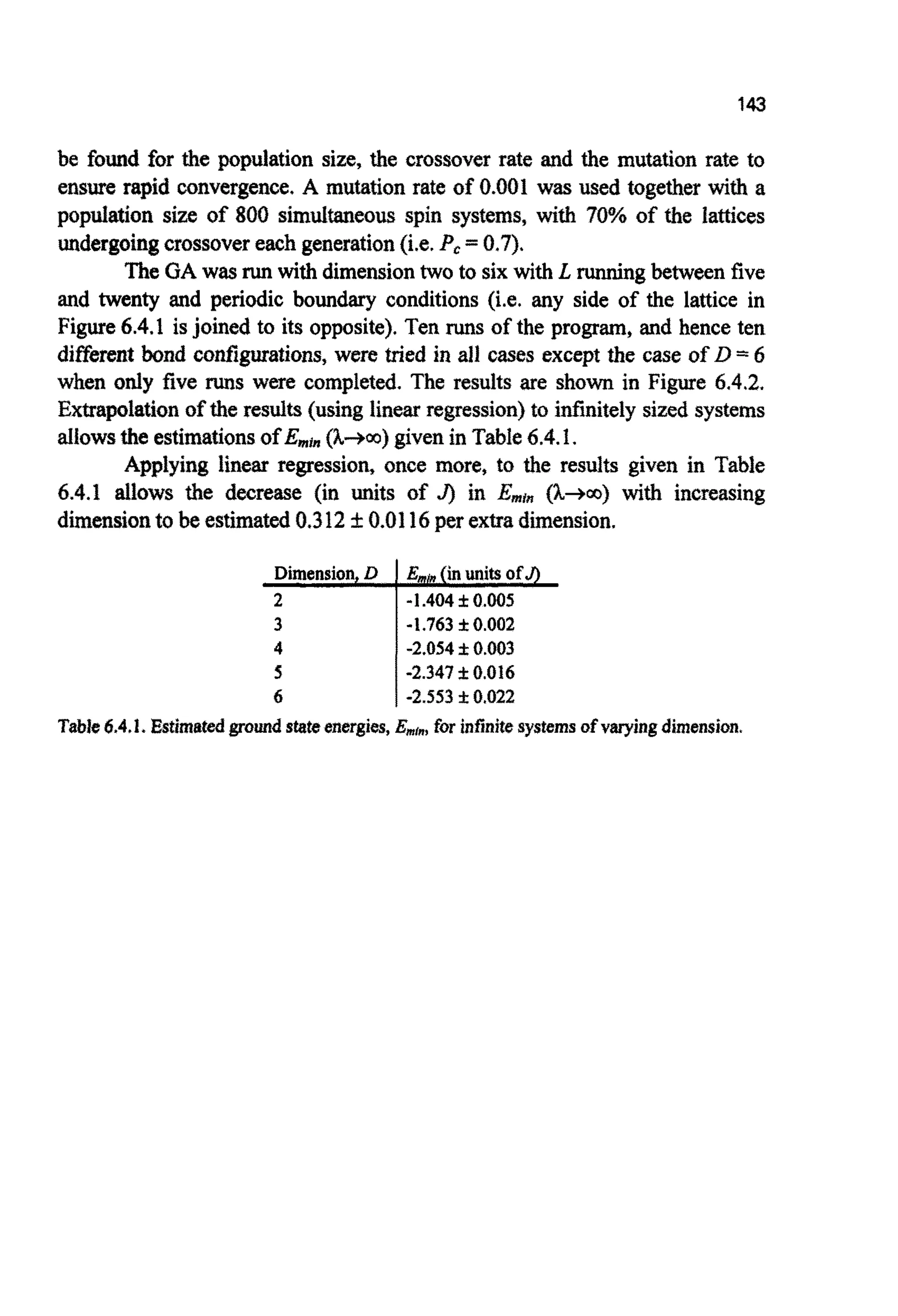
161. 144
0.05 0.10 0.15 0.20 0.25 0.30 0.35
1/L (Vsystem length)
Figure 6.4.2. The calculated ground state energies, together with their standard errors, of the
differentsystems(linesestimatedby linear regression),from [WA96].
6.5 ESTIMATIONOF THE OPTICAL PARAMETERS OF LIQUID
CRYSTALS
Liquid crystals are finding an increasing number of applications from watches
to complex displays for portable computers. This utility arises from the ease
and speed with which the molecules within liquid crystals can be made to
reorientate themselves. Interestingly, the precise orientation as a function of
depth is not fully understoodfor many systems.
The best methods currently used to study this orientation
[YA93,YA93a]rely on laborious hand-fitting of experimental data to a model
of the system. Recent attempts to automate this process using a GA
[MIK97,MIK97a]have proved highly successful. In order for the approach to
work, a series of adaptations to the simple GA are required, and the approach
illustrates much of the wrestling often undergone to produce a successful
application. In particular,the followingare considered:
the developmentof a systemto replace a previouslyhuman-guidedsearch;
how, starting from a simple problem, a series of sequential adaptations are
made;

162. 145
the use of iinear fitness scaling, bound reduction, fitness function
a ~ p ~ t i o n s ,approximate fitness evaluation and a variable mutation rate;
and
0 the inclusion of a traditional searchroutineto create a hybrid algorithm.
LIQUIDCRYSTALS
Liquid crystals exist in a series of states of matter somewhere between the
usual solid and liquid states. They have been investigated since the 1880’s
when Reinitzer and Lehmann first studied esters (benzoate) of cholesterol.
Unlike the usual states of matter, they display a series of “mesophases”,each
of which has distinct structural properties categorised by the degree of
positional and orientationalordering found within them. It is the existence of
these mesophases,and the possibiIi~of makingt r ~ ~ t i o n sbetweenthem, that
have allowed liquidcrystalsto be deployedin a range of technologies.
The characteristic feature which links the many thousands of
substances,both naturally occurringandmanmade, that show liquid crystalline
phases is that the molecules are anisotropic:either elongated, cigar-shaped or
disk-like. The anisotropy of the moleculesis reflected in i n t e ~ o l e c u l ~forces.
It is these anisotropic forces which lead to the formation of the numerous
mesophases.The averagedirectionof the principal molecularaxis is givenby a
unit vector, or director. As the temperature of a liquid crystal is reduced
increasingorderis gained.A typical sequencewould be:
isotropic,which has no longrangepositionalororientationalorder(i.e. liquid like);
5-
nematic, which has no positionalorder ,but someorientationalorder;
5-
smecfic, which has both positionalandorientationalorder;and
5-
rryslal, whichhas highpositionalandorientationalorder.
Many phases are chiral, i.e. the director precesses as you move through the
material.
Not only are such molecules physicaliy anisotropic, they are also
d i e l ~ ~ c a l l yand optically anisotropic.As a result, if an electricfield is applied
alignment of the molecules will occur. This potential for alignment is at the
heart of such materials being usekl in display technologies. The optical
anisotropyresultsin differingeffectiverefractive indicesfor polarisationalong,
andperpendicularto, the molecularaxis.

163. 146
Sandwichingthe liquid crystal as a thin layer between two glass plates
that have rubbed polyamide coating their inner surfaces is enough to physically
align the liquid crystal along the rubbed direction. If the glass plates are first
coated with a transparent conductor then, once assembled, an electric field can
be applied to re-orient the liquid crystal. Furthermore, if this cell is placed
between crossed polarisers the alignment of the liquid crystal will effect the
transmissions of lightthrough the cell, resulting in a simple display system.
In a typical, standard, simple twisted nematic cell, about 1O p m of liquid
crystal is placed between the plates, with the alignment layers used to impose a
90° twist on the directorthrough the cell. Incident light is then naturally guided
(twisted) as it passes through the cell and is able to exit through the second
polariser. Applying an electric field (of the order of lo6Vm-') induces dipoles
in the liquid crystal molecules which align in the direction of the field, stopping
the light from emerging from the second polariser. Removing the field returns
the cell to its original state.
If a liquid crystal cell of low order is mechanically deformed,
birefringence colours become visible, but once the deforming force is removed
the molecules flow back to regain their original structure. However, in highly
ordered systems in more solid-like mesophases, the structure of the system is
left permanently deformed, making the device useless as a display. If more
were known about the details of the exact structure within such cells (with and
without defects) progress might then be made on better cell designs. Work by
Mikulin, Coley and Sambles using GAS[MIK97,MIK97a]has been centred on
detailing this structure.
THEHALF-LEAKYGUIDEDMODETECHNIQUE
The principal optical tool for the study of liquid crystals is that of optical
polarising microscopy. Because this technique integrates the optical response
through the entire thickness of the cell, only some weighted average of the
director orientation is obtained. In order to understand the underlying structure
within the cell, a method that can detect details of the spatial variation of the
director is required. The development of optical waveguide techniques, in
particular the use of the Half-Leaky Guided Mode (HLGM) technique by Yang
and Sambles [YA93,YA93a],providesjust such a method.
A waveguide consists of a sandwich construction, such as a fibre optic,
where a core of high-index glass is surrounded by glass of lower index. The
difference in the refractive indices can ensure, under the right circumstances,
that the light is contained within the waveguide. The light in such a waveguide
mode follows a zigzag path within the central medium. Many such paths or

164. 147
modes are possible. In many ways these modes are similar to organ-pipe
standing waves. The lowest energy mode that can be excited is the
fundamental, which has averaged electric field distribution nodes near the
waveguide surfaces and a maximum in the centre. Higher energy modes are
harmonics where progressively more half-wavelengths fit into the waveguide.
The maxima for each of these harmonics are seen to occur at different positions
within the waveguide. By building a waveguide consisting of a liquid crystal
layer, the optical excitation of the guided modes which may propagate in the
cell may be used to characterise the liquid crystal optical parameters as a
function of position within the cell. In particular, measuring the angular
dependence of reflectivities which characterise resonant modes provides data,
which when compared to a mathematical model of the cell gives the director
profile through the cell.
In practice, polarised monochromatic laser light is incident (via a
prism) upon the cell which sits on a rotating table. A photodiode detector is
used to detect reflected light, and an oven enclosure is provided to allow the
study of various mesophases. The incident beam can be either p- or s-polarised
and the detector is arranged such that only p- or s-polarised light is detected.
This means that four possible angle-dependentdatasets of reflected light can be
collected: Rpp(p-in, p-out); R, (s-in, s-out); Rps (p-in, s-out) and R, (s-in, p-
out). A typical data set contains measurements made at about 1,000 different
angles.
THESEARCHSPACE
The mathematical model used of the cell is based on Fresnel’s equations of
reflection, and views the cell as a series of discrete optical layers. These layers
correspond either to real physical layers in the non-liquid crystal part of the
cell, or arbitrary sub-layersof the liquid crystal chosen such that any individual
layer is optically thin. The number of sub-layers required to accurately
represent the liquid crystal depends, in part, on the complexity of the liquid
crystal mesophase in question. As the number of sub-layers grows, the
numbers of unknown adjustable parameters (used to describe how the
moleculesbend and twist the light) in the model also grows. Attempts to find a
traditional search method capable of adjusting these parameters, so as to
minimise the difference between the experimental data and predictions from
the model have failed because of the complexity of the search space. This has
meant that such fitting is typically carried out by a human-guided search
through the space with intermittent use of a gradient-based search algorithm.
Such a search may take severalman-months.

165. 148
The complexity of the search space arises from the large number of
parameters(typicallymore than 50)which are being adjusted and the existence
of a very large number of local optima throughout the space. This results in
many combinations of parameters leading to similar traces. One way around
this problem is to attempt to fit more than one dataset, i.e. Rpp and Rss at the
same time. This removes many of the degenerate solutions because some often
prove much poorer solutions for the second dataset. Another possibility is to
change the ~imuthalorientation of the cell relative to the pol~sationof the
incident laser beam and collect new data sets. Given enough data it should be
possible both to navigate through the space more effectivelyand also locate a
definite global optimum. However there are problems with such an approach:
the more data the better the fit, but the bigger the search. This is a general
problem with many experimental datasets. Collecting more data makes the
topology of the modelled search space closer to the physical problem space,
smoothingoutmany irregularitiesand, hopefully, allowingthe identificationof
a globalo p t i m ~ ,but only at the cost of a much largerproblem.
In the HLGM data, if there are Rpp,R,,,Rps and R.Ipsets at 1000angles
and two azimuthalangles,then the computermodel will have to make 4 x 1000
x 2, or 8000 estimationsof the reflectivity for a single guess at the ~o~
parameters, making it impossibleto consider random or enumerativesearches
and difficult for any other method. These problems---of a complex search
space together with computational time constraints-have meant that it is
considered impossible to successfully fit such datasets, and thus impossible to
fully characterisesuch cells.
The use of a GA on the problem proved highly effective, but not
without difficulty. The first GA applied was very simple indeed. A binary
encoding was used (with 10 bits per ~ o ~ ,i.e. I, =4, i #j)together with
rank order selection (with the best 50% of individuals being selected for
crossover once and only once) and random replacement by children of the
original population members to create the new generation. Mutation was
applied, at a rate of 0.001 per bit per generation, across the complete new
generation, and elitism applied. The fitness measure used to distinguish
between solutions was based on the sum of squares (SOS) differencebetween
the experimentaland modelled data:
where

166. 149
i-I
where R isone of the ~flectivitiesRpp,R,, Rpsor Rspand p is the theoreti~ly
predicted (i.e, modelled) reflecti~~.The sum is carried out over all data
points, or angles, 8. The constantA is selectedto be equal to or slightly greater
than any likely value of SOX On the odd occasionwhen a negative fitnesswas
produced, the fitness was set equal to zero. The results proved surprisingly
good for a first attempt. Typical initial values of SOSof 200 were reduced to
0.23 within a few hours on a fast personal computer for a nine parameter
nematic (i.e. relatively simple) cell problem and gave parameter values very
close to those found by laborioushand-fitting (an approachwhich might take a
month for suchdata if similarboundswere used).
Initially, attempts to study more complex cells with 27 unknowns
failed. When presented with both Rppand RPs data at two azimuthal angles,
where the m i ~ m ~value of SOSwas known to be approximately lo", only
SOPSof somethingless than 10were achieved. In orderto make the approach
useful for characterisingmore complexcells,a seriesof adaptationswere made
to the algorithm.
REDUCING THE STRING LENGTH
The fa improvement tried was to assign different binary word lengths to
different parameters. This very basic adaptationwas felt to be sensiblebecause
different parameters were known to affect the goodness of fit to varying
degrees. This is probably crucial for a GA to work effectively with a large
number of ~ o w n s .A simple GA with a stringlengthof severalt h o ~ ~ dis
likelyto take a very longtime to convergewithin most real searchspaces.
Such an approach rapidly reduced (in c 100 generations) the SOS to
less than 1. However, progress past this point proved very slow. One reason
appeared to be that for SOS< 1, many of the strings have bit-patterns very
close tothe pattern they would have at the global minimum. At such a point it
becomes very difficultfor a GA (with large L)to progress by simplecrossover
and mutation to the global optima. In particular, mutation will almost always
be destructive and the search becomes close to looking for a needle in a
haystack. Unfortunately switching to a traditional search mechanism at this
point could still not guarantee locating the global optimum. One approach to
this problem proved to be the sequential use of the GA within a narrowing
search space. This ensures an efficient gridding of the search space by the
binary encoding.A sketchof the method is givenin Algorithm6.5.1.

167. 150
1. Apply GA until the solution no longer improves or for a fixed number of
2.Reducethe sizeof the search space and re-initialise the GA
3, Repeat from I a set number of times, or until convergenceis reached.
generations.
Algorithm 6.5.1. A GA with bound reduction. Note that such an approach is not suitable for
most types of search space and care has to be taken not to exclude regions of the search space
too early.
Step 2 of A l g o r i t ~6.5.1, the reduction of the size of the search space,
could take one of many forms. The simplest would be to reduce the width of
the space for each unknown by the same fractional amount, giving a new space
centred upon the current best solution. This could well cause problems. For
example, if the old space had width w,, for parameterjand the new space is to
have width w; = wJf2,then if the current best guess of parameter] is closer than
wJ14to the upper or lower bound of the original space, then the new space will
include a fragment outside of the range initially specified as the problem space.
At best the inclusion of such a fragment is wasteful, at worst it may
lead to the production of an unfeasible solution. One way around this is not to
allow any new bound to fall outside the initial search space, and if it attempts
to do so,to simply give it the value of the initial bound.
Another question to be answered is the size of the reduction constant n,,
where:
The greater the value of PI,the faster, but the less reliable, the convergence.
One possibility is to make n, dynamic and base its value on the value of a, (or
some other statistic) estimated from a single run or a series of runs of the GA.
This could occasionally allow n, < 1 (i.e. an expansion of the space). If all runs
progress to similar values of a parameter then a greater reduction in the size of
the search space is possiblyjustifiable. However, extreme caution is required to
make sure that at no point is the true global minimum excluded from the search
(this will not be possible for many search spaces).
Using such an approach on the HLGM data proved very successful,
with the SOS rapidly being reduced toward zero (Figure 6.5.1).

168. 151
Figure 6.5.1. Enhancing the GAS performance by repeated bound reduction (data from
[MIK97a]).
In essence, such bound reduction is a~emptingto make the crossover
and mutation operatorsequally effectiveacrossall unknowns, regardless of the
sensitivity of the problem to a particular parameter. Hence for parameters
which initially have littleeffecton the fitness, the boundswill remain wide; for
the morecriticalonesthebounds will slowlyreduce. There are many functions
for which such an approach is unlikely to be suitable and will flounder.
However, within spaces characteristic of several physical problems where a
solution can be incrementally zoomed in upon it may be successful. An
example of the successful performance of the method on theoretically
produced HLGM data for a liquid crystal in the nematic phase is shown in
Figure6.5.2.

169. 152
7
10-
0 8 -
Q o 6 -
$ 0 4 :
0 2 -
0 0 -
-
, . , , , . ~. , , , , , . , .0 5 - 5 4 16 5% 60 61 64 66 68
Figure 6.5.2. The performance of the sequential GA on the relatively simple problem of
nematic HLGM data with 27 unknowns: cross = data, line = fit) (data from [MIK97a]).
APPROXIMATEFITNESSFUNCTIONEVALUATION
As has been suggested before, the time it takes for a GA-based optimisation
routine to cycle through a generation is likely to be dominated by estimations
of the fitness function, rather than the genetic operators. In the case of the
HLGM data this means that the computing time required is proportional to the
number of data points. However the accuracy of the final answer will, in some
complex way, be a function of the number of data points. So a conflict exists
between speed and accuracy.Or, put another way, given a fixed (or reasonable)
amount of time for the running of the program, how can accuracy be
maximised? Is it best to estimate the fitness function as accurately as possible
and reduce the number of generationsprocessed, or would it be better to use an
approximation to the fitness function (which can be estimated more rapidly)
and process more generations? The answer to this question is obviously
problem-dependent. It is also likely to change during the optimisation process
itself. During the early stages of the search, fitnessesare likely to be low and so
their accurate estimation is unlikely to be important. However, at later stages
navigation of the algorithm through the search space is likely to rely on subtle
differences in the fitness function in differentdirectionsof the hyperspace.

170. 153
To try to speed up the search, and thereby ultimately allow for greater
accuracy,the HLGM data was filteredto only leaveP!of the data points. As
the run progressedthe value of D was increased. For the HLGM data the form
D =D(g) was used; however D =D(f) would possibly be more natural. With
this approach, it was found possible to quarter run times for no loss of
accuracy.
USEOFFITNESSSCALING
As discussed in Chapter3, GAScan experienceproblemsif the fitnessfunction
spanstoo little, or too great, a range within any one generation.In particular, if
during the early stages of a run a small sub-population (typically of size= 1)
has individualswith a much greater fitnessthanthe populationaveragethen the
sub-~p~ationcan rapidly grow under ~tness-propo~on~selection to
dominate.Thiscan lead to prematureconvergence.Conversely,duringthe later
stages, a large sub-population (typically of sizemiV) may only contain
individuals who have fitnesses approximately equal to the population
maximum. In such a situation, simple fitness-proportional selectioncan make
little distinction between sub-population members and the progression of the
algorithm is muchreduced.
Linear fitness scaling was used on the HLGM problem to control the
expected number of times above-average population members would undergo
selection, compared to an individual of average fitness. A range of values for
the multiplieremwas tried and an improvementin convergencenoted, Making
c, dynamic, i.e. c, =c,V) or Cm =c&) wasnot tried.
DIRECT FITNESSFUNCTION ADAPTATION
Unlike many problems where few details of the functionalform of the search
space are known prior to optimisation, partial enumerative searches through
~ e o ~ t i c ~data had produc~insightsfor somecells, In particular, many of the
unknowns had been found to show sections through the solution vector that
contained large areas of equal fitness nearf. Such a section suggests the
substitution:
f = f" ; m >1 ,
might be of benefit. Such direct scaling can only be applied if some of the
detailsoffare already known (allowinga sensiblechoice of m).

171. 154
For the HLGM problem several values of M (m= 6 proving the most
useful) were tried and again improvement in convergence witnessed across
many setsof data. (Similarresults could have been realised by making suitable
a d j ~ ~ e n t sto the selection mechanism itself, because fitness ~ c t i o n
adaptation and fitness scaling are two sides of the same coin. However, it is
often more naturally intuitiveto adapt the fitnessfunctiondirectly.)
~ U Z ~ Z ~ GTHE ~OPULATION
Long periods of only marginal, or no, progress were seen during many funs
with some cells. An attempt to see if the computer time during such periods
could be better spentwas made by making the substitution
In essence the population was boiled, whilst main~iningelitism, by
momentarily (typically for three generations) increasing the mutation rate. It
was hoped that not only would this encourage diversity within the population,
but also allow the population to jump over traps in the binary representation
caused,in part, by not implem~ntinga Gray coding.
In order for such an approach to effect the diversity of the population
for more than a few generationsafier the boiling event,fitness scalingmust be
applied simultaneously.Without such scalingmost individualsproducedby the
operation will be lethals (except the elite member) and fail to be selected for
subsequent gene~tions.This reinforces the idea that additional GA operators
cannot be used in isolation and without regard to those operators (and their
settings)already in use by the ~ g o r i t ~ .
ADDITIONALDIRECTSEARCH
In line with the comments made in Chapter 1, many problems are likely to
benefit from the inclusion of a traditional search algorithm working in
combinationwith the GA. In this casethis was done by the inclusionof a direct
searchmethod proposed by Jeeves and Hooke [BU84], al~oughother methods
could have equally been used. The direct search was applied (to data Erom the
highly complex smectic C* phase with 55 unknowns)afterg = G in an attempt
to climb the final hill. This was successful, with the improvement in fitness
being far in excess of that which might have been expected from a similar
numberof add~tional~ c t i o nevaluationswithin the GA.
The final (and most successful) algorithm used in this work can be
described by the schematic given in Algorithm6.5.2. The algorithm was

172. 155
arrived at by trial and error based on an extensive knowledge of the macro-
details of the search space but has little justi~cationother than it works
extremely well for the problem at hand. If such knowledge had not been
available, then some of the settings within the algorithm might have been
discovered by including them in the search space, using the techniques
described in references[GR86, BR91, DA89 and DA911.
1.Run GA with G = 30, n =60, P, = 0.5, P, = 0.0016, linear fitnessscaling,
fitness-proportionalselection with elitism, and using the minimum sub-
stringlengthsrequiredto maintainaccuracy.
2.Boil population, maintainingthe elite member.
3.Repeat steps 1 and 2 six times.
4.Reduce the bounds on the parameters to 120%of the spread of values of
5.Repeat from 1 fivetimes.
f- (G =g) obtained from the six GA runs.
6.Apply directsearch.
Algorithm6.5.2.The final algorithmused with the HLGM data.
This algorithm is a long way from LGA and indicates that GAScan
benefit greatly from adaptations that attempt to include additional knowledge
about the search space in question. The success of the method can be gleaned
by the closeness of fit shown in Figure 4.5.3, which shows a fit to the much
more complex smectic C* phase. Figure 6.5.4 shows the liquid crystal
molecular orientations discovered by the GA: the molecules are seen to
graduallytwist and tilt throughthe depthof the crystal.

173. 156
Figure 6.5.3.Fit (line) to experimentalsmectic C*data (at 21'C) (+) with 55 unknowns (data
from [MIK98]).
94 16
92 -
8 6 , 7 , . , . , . , . , . 6
0.0 0.5 1.o I S 2.0 2.5 3.0
Depth(run)
Figure 6.5.4. The twisting(e) and tilting ( 0 ) of the molecules through the depth of the crystal
discoveredby the GA (pointsconnectedby 8-splines)[MIK98].

174. 157
6.6 DESIGNOF E ~ R G Y - E ~ c ~ ~BUDKNGS
Considerable scope exists for reducing the energy consumption of both new
and existingbuildings.
Although some reductions in energy use can be achieved by relatively
simple measures, very high levels of performance require the coherent
application of measures which together optimise the performance of the
completebuildingsystem. In essence,the designer, who will typicallybe more
of an architect than a scientist or engineer, is faced with a multi-component
optimisation problem. Most designers feel ill-equipped to tackle such a task
and thisis a seriousobstacleto them advancinghigh performance designs. The
application of computerised optimisation techniques to the design of low
energy b ~ l d i ~ scould provide architects with a powerful new design tool.
With the increasinguse of graphicalpackages duringother stagesof the design
progress such an approach could eventually be included within the design
environment,
Population-based optimisationappearsto be ideally suited to providing
the type of support and assistance needed. Most traditional optimisation
t e c ~ q ~ stbat might be applied sufier fbm the drawback that only a single
result is obtained. Because of the difficulty of including such factors as
aesthetics in the optimisationprocess (as discussed in Chapter4), it is likely
that any “optimum”resultwill be found to be unacceptable.
Giventhe numberof individualattributesthat combineto make a single
build^^ the number of possible realisations, or designs, is very large. Work by
Migowsky [MIG95] showed that a GA can be used to allow a rapid and
efficient searching of this multi-dimensional building space. The method
produces not only the near-global optimum, but ah0 a set of high quality
designs. Each has excellent energy performance, but the set is sufficiently
diverse in physical c h ~ t ~ s t i c sto allow the designer the opportunity to
select on the basis of other i m p o ~ tnon-optimised criteria. A GA can thus
formthebasis for apowerfulandpractical buildingdesign aid.
The system allows a designerto select from a range of buildings,all of
which have a predicted energy performance within, say, five percent of the
achievable minimum, the design which best suits hislher other requirements.
”his a ~ ~ his in line with the establishedpreference of architects to work
fromcasestudy and demonstrationmaterial. It relievesthe designerof the need
to work through the consequences of choosing individual features and of
checking their compatibilitywiththe rest of the building system. The architect

175. 158
is instead offered a selection of optimised, complete, building packages from
which to make a selection.
The complete system has a pair of criteria to be satisfied: first a
numerical measure of fitness which can be used to drive the GA, and second, a
qualitative assessment of the aesthetics of the design to which it is impossible
to attach a numerical estimate. Because this second measure is non-numerical,
Paretooptimisationmethods (see 34.4) are not suitable.
Although the energy model used in this work contains only five true
unknowns, it is impossible to describe or visualise a building with only these
parameters. The building must be considered as consisting of a far greater
number of parameters (>loo) which are far from linearly independent. In
essence, the GA is being used to throw up ideas, good ideas, because they are
highly energy efficient,but still only ideas.
In the work described here, which is taken from developmentsbased on
reference IMIG951, the approach is applied to the design of a set of school
classrooms. The work shows an example of a problem with the following
features:
a range of differentvariable types (binary,integer and real);
the need for a diverse range of approximate solutions together with the
global optimum;
the need for human-based final selection;
a large multimodal space studied by using multipleruns;
a highly non-linearly independent search space;
because of the time taken to evaluate a single design, the need to avoid re-
estimatingthe fitnessof any previously processed design;
remainder stochasticsamplingto help reduce the convergencerate; and
use of a generationgap.
INTRODUCTION
Up to fifty percent of the United Kingdom’s consumption of fossil fuels is
related to energy use in buildings. The burning of fossil fuels, and the
associated emission of combustion products, contributes to global warming,
acid rain and other local pollution.
The energy performance of a building is determined by its responseas a
complete system to the external environment and the internal environmental
demands of the occupants. The system response, in turn, depends upon the
combination of individual attributes that have been assembled to produce the

176. building. Thus, for example, a building with large windows, lightweight
structure, elongated form and a powerful heating plant may be more, or less,
energy-successfulin the role of a primary school than one with a differentmix
of features. Traditio~ly,a solutionis proposed on the basis of experience and
on the evidenceof the ~rformanceof other demo~~ations.The perfbrmance
is then checkedusing predictivemodels, and the design may be adjusted in the
light of the results. By this means, an acceptable solution is arrived at-but
there is no practical way of determining how close to a realistic optimum the
final designis.
Unfortunately for the designer, it is not possible a priori to say which
detailed combination of attributes represents the best solution to a particular
brief. This situationarises because, although the performance of any particular
system can be predicted using a suitable mathematical model, the inverse
probfern of determining the optimum system characteristicsfrom the desired
performance cannot be solved. Optimisation is therefore a process of trial.
Given the number of in~vidualphysical ~ ~ b u t e s~ r n ~ ~ s i n ga single
building, the number of possible combinationswhich results fromvarying each
attribute over its range of practical values is enormous. This precludes direct
modelling of the entire building set and indicates that the multi-dimensional
buildingparameter spacehas to be searchedin a more efficientmanner.
The main characteristicsof the problem are a large multi-dimensional
space to be searched, requiring an efficient method to converge within a
reasonabletime; a multimodalspacerequiringtechniquesto avoid convergence
on falseminima; a requirementnotjust to identifya singleoptimum result, but
to also map the positions of a range of lowest energy solutionsthroughout the
space.
Themethoddescribedin reference [MIG95] uses energy predictionsfor
individualbuildingsmade using the buildingthermal simulationEXCALIBUR
[CR87a, CR87bJ. However, any other proved thermal modelling approach
(manyof which are far moresophisticated)would be suitable.
THERMALMODELLING
The five-parameter computer model of the thermal response of buildings
developed at Exeter, EXCALIBUR, has been used to aid the design of over
seventy large buildings, from schools to underground military facilities. The
success and continuing utility of this model has codirmed the original
conviction that the essential features of building performance, in terms of
internal temperature evolution and total energy usage, can be adequately
representedby a l ~ ~ - p ~ ~ e t e rdynamic model. This approachresults in a

177. small portable program capable of running quickly on desktop machines. The
model is based on a two time-constant analogue circuit with five adjustable
parametersper heated zoneof the building (Figure6.6.1).
Figure 6.6.I. The electrical R-C analogue of a single EXCALIBUR mne.
The characteristicequationsare:
where kt represents a quick response thermal conductance (ventilati~nheat
loss, window losses etc.) between the inside temperature node T, and the
outside temperature To;ki is the thermal conductance between Tj and the mid-
structural temperature T,; ko is the conductance between T, and To;c, is the
effectivethermal capacity of the air; cwthe thermal capacity of the structure of
the building; and q the heat supply (including metabolic, lighting and other
gains) actingat T,.
These equationsare solved analyticallyand the model building is time-
stepped through a complete season of representative weather data, including

178. 161
angle dependentsolar intensity. Realisticoccupancyand temperature schedules
can be specified and the user can choose between manual and optimum-start
plant control. The program can accommodate up to ten thermally linked and
separatelycontrolledzones.
Themodelthereforeprovides the meanswhereby reliablepredictionsof
seasonai energy use can be made for buildings with any reasonable
combinationof physical attributes.However,such a model suffersfrom at least
one major setback: few architects (or building scientists) would be able to
visualise designsin terms of the model’s parameters, V“& (i.e. cw,k, etc.). The
designer is using the much larger set of physical attributes, such as
positions, wall lengths, material types, etc, fiom which the five model
parameters per zone are estimated. Many combinations of physical attributes
will give rise to near identical combinations of model parameters. Many
attributes are highly related-the perimeter and the enclosed volume for
example). The search space is therefore highly m~timodaland chocablock
with non-linearly independent variables. The scale of this problem can be
illustratedby the realisationthat the searchspacemay contain in excessof one
hundred unknowns, yet the model containsonly five.
THEPROBLEM
Theproblem at hand is that of finding diverse sets of vectors V‘&’ such that the
energy use of the building over a year is near minimum. The ideal value, Tjer,
of the internal temperature, Ti,during occupancyis set by the designerand the
amount of energy required to maintain this value will depend greatly upon the
design. The building gains “free” heat &om solar input through windows,
metabolic gains from the occupants and gains h m electrical equipment (for
examplethe I i ~ t ~ gsystem^. If these gainsare i n s ~ ~ c i e n tto provide Tst then
additionalinput is provided by the heating system.If Ti> Tsefheat is removed
by thc cooling system. In a low energy building, the need to provide such
additional gains must be kept to a minimum. This position is achieved by
“minimising” losses (ko,k,,kr) and “maximising” the use of free gains. The
thermal capacitance of the building fabric is then used to try to time-table the
match between supply and demand. Unfomately, this proves to be a fine
balancing trick. If solar gains (for example) are truly maximised and losses
simultaneously truly minimised, the building will fiequently overheat,
requiring the expenditureof largeamountsof coolingenergy.
The loss terms (he, ki, kl) and the thermal storage terms (cw, ca) are
formed &om a complex ~mbinationof the building components. This list of
componentsis extensive. A singlewall typically containsmany layers: external

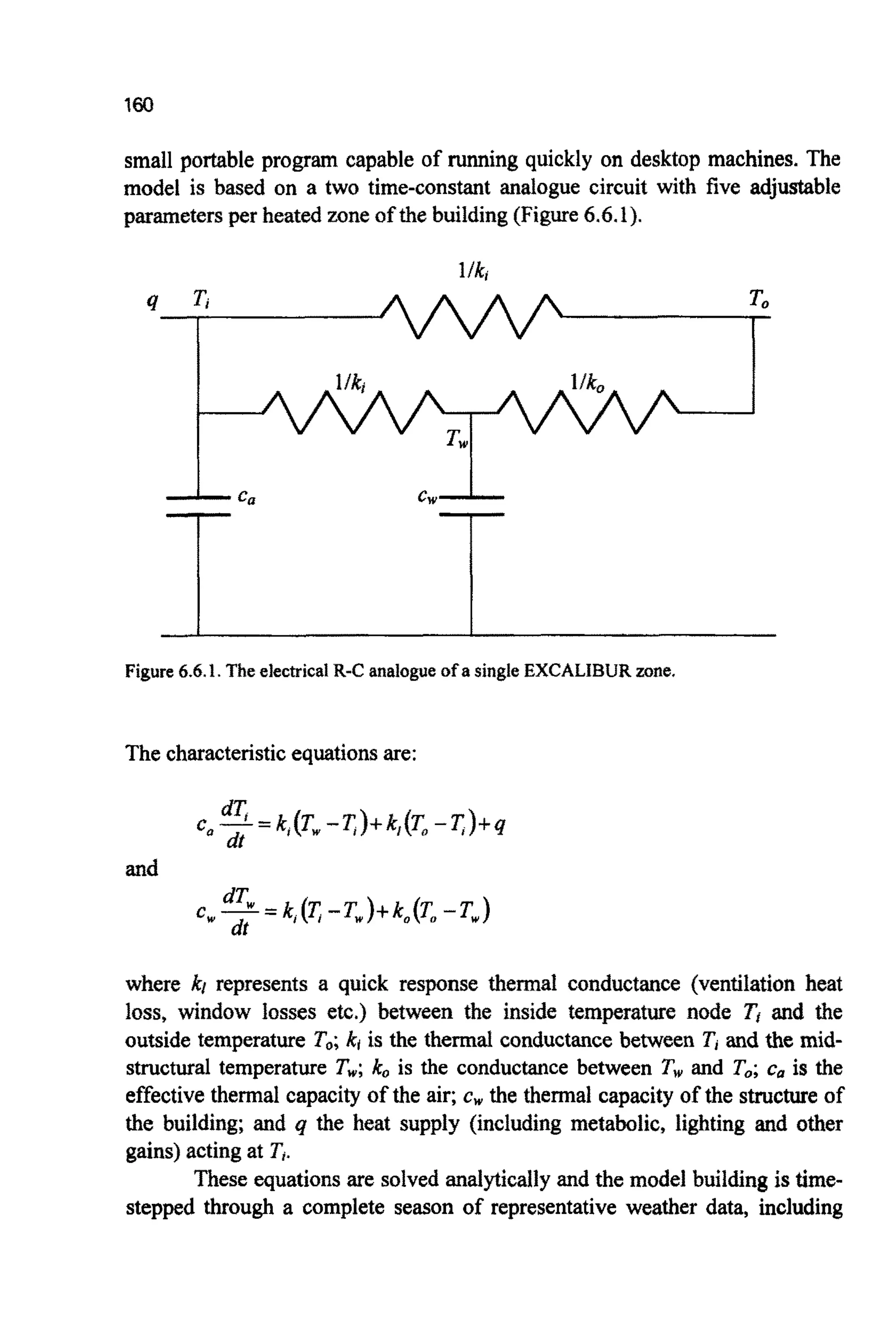
179. 162
brick, air gap, insulation, inner concrete-block layer, and plaster. Both inner
and outer walls have to be considered, as do the floors and the roof.
EXCALIBURtakes a single combinationof these components as specifiedby
the designer, forms a single set of model parameters (kQ,k,,kr, c,, ca), then
combinesthese with an occupancy schedule and cycles the building through a
year of weather data whilst using the heating and cooling systems to ensure
Ti= Tserduringoccupiedhours.
In the work of Migowsky [MIG95], and subsequent extensions,
EXCALIBUR is combined with a genetic a l g o ~ t ~to try and generate high-
quality designswith architecturalappeal.
The population,P,is manipulatedas follows:
1. create initial,random, populationof attributesP(yphys);i = 1...N;
2. reducephysical attributesto model parameters y@ys-+ F”’&;i = 1...N;
3. calculateannualenergyuse of heating and coolingsystems,Ei ;i = 1...N;
4. use GA to create new designs PhYsby recombination and mutation using
f=A -E (whereA is a positive valued constant)as the selectionfactor;
5. repeat from 2 until terminationcriterion is met; and then
6. filter designsconsideringarchitect~alappeal.
It should be noted that human judgement is only applied after g= G,
not, as in the examplepresented in $6.7, where suchjudgementsare the driving
forcebehind the GA’s selectionmechanism.
The success of the GA phase can be gauged from Figure 6.6.2. Here, a
small extensionto a primary school is being designed. The annual energy use
of the building rapidly falls with generation,and the final design is seen to be
far better than is typical for such structures.
REPRESENTATION
Each VhYsis represented as a binary string. As some parameters are reds (e.g.
“ ~ u i ~ ~ i n gp e ~ ~ e ~ e r ” ) ,some are integers and others are ~ o o ~ e ~fe.g. “double
or single glazing”), the substring length I for each parameter varies greatly.
This implies that the mutation and crossover operators interact with some
parameters more frequently than others. If I is chosen to truthfully reflect the
required accuracy of each parameter, this probably presents no problem
because the degree of int~ractionis then propo~ionalto the required accuracy.
However if each I is not selected with care, then the algorithm will spend a
considerable time processing irrelevant information. For example, if the wall

180. 163
thickness is only specified to the nearest cm, then there is little need to specify
the building perimeter to the nearestmm. In reality, the correct set of sub-string
lengths can only be identified given enough experience of the likely impact of
each unknown on E, and knowledge of the commercially available sizes of
constructionalcomponents.
POPULATIONDIVERSITY
As the desire is to find an extensive range of possible designs, not just the
optimum, population diversity must be maintained throughout the run. The
algorithm used is a simple GA and therefore does not include niche and
speciation methods; thus the selection and mutation operators must be relied
upon to perform this role.
Selection is via remainder stochastic sampling (which places a limit on
the number of times any individual can be selected) with a generation gap (see
Chapter4). Mutation is applied only to the children, which replace at random
individualsin the originalpopulation.This approach is found to simultaneously
maintain diversity and remove low quality designs rapidly. A population size
of 50 and a generation gap of 0.8 are used.
AVOIDINGDUPLICATEFITNESSEVALUATION
The evaluation of E, for all i is time consuming, especially on the type of
machineto which a building designer might be expected to have access. Thus it
is crucial that designs are not re-evaluated. This is simple to achieve: a list of
all unique designs, together with their respective value of E, is kept and new
designs checked against this list. If a match is found then the corresponding
value of E is simply assignedto the new individual.
This list-keeping process, or something similar, is probably worth
including in many scientific or engineering-based applications of GAS. Only
for the simplest of problems (typical of those used as test functions) is it likely
that searching the list will take longer than a single fitness evaluation. By
searching the list in reverse order (assuming new designs are placed in at the
bottom) and not searching for any member which has not undergone crossover
or mutation (because its fitness will not have changed), efficiency can be
further improved. For long lists, it may prove desirable to only keep and search
designs from relatively recent generations.
Although a reasonable level of genetic diversity is maintained during
early stages of the run,Figure 6.6.2 shows that this diversity is not maintained
throughout the run.Here the number of matches that were found between the
current population and the ordered list is being plotted. (The algorithm never

181. 164
truly converges, which would be indicated by fifty (i.e. N) matches in any
generation, because of the relatively high levels of mutation used.) It is thus
clear that if this work is to be continued, additional measures will have to be
taken to increasethe degree of exploration in the go^^ during these later
stages-possibly by never allowing two individuals within the current
generationto be identical.
40 -I
t t f t
0 so 100 150 200
8
Figure 6.6.2.The number of matches (out of fifty) found between the current population and
the ordered list of designs. Convergence{s~gnation)is avoided by the use of relatively high
mutationrates.
THEADDITIONOF ARCHITECTURALAPPEAL
The problem presented is a multicriteria one, requiring, at least, the
mi~misationof energy use and the m~imisationof architectural appeal, No
attempt has been made to include this appeal in the selectionalgorithm,and it
is not clear-even using Pareto optimality-how this could be achieved
without greatly reducingthe numberof processeddesigns.
As an alternative to even a~emptingthis, ~igowskyuses a filtered
stacked histogram to present the best designs. The list of all designs
(Figure6.6.3) is initially filtered to remove all with a value of E more thanv%
greater than the best. (Typically v = 5 to lo%.)By using S>>1 the regions
around many local optima are included in this set (see $4.2). A stacked
histogram of these unique designs is then presented on Screen for the designer

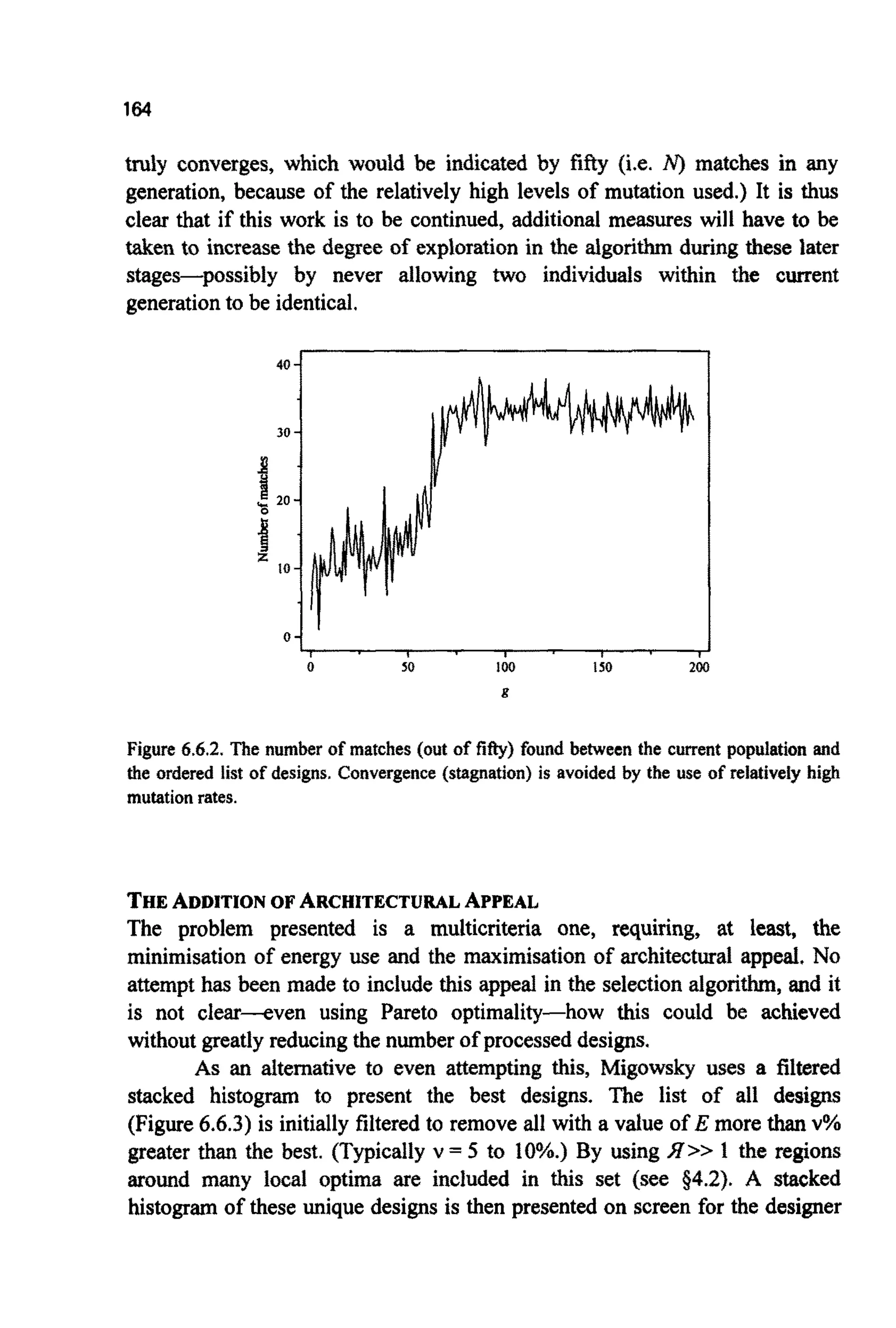
182. 165
to study (see Figure 6.6.4 for a fragment). A select few of these designs can
then be worked up to sketches(Figure 6.6.5).
The two designs shown in Figure 6.6.5 have relatively similar annual
energy usage, but are of very different design. One uses high levels of
insulation to reduce losses, the other maximises solar gains. Interestingly,
combining these two design philosophies within a single building does not
produce a high performing structurebecause it would overheat on sunny days
(and thus have reduced fitness). The method is highly successful,not only as a
method of obtaining high performing designs, but equally importantly,
catalysing the design process by showing that similar environmental
performancecan be achievedin a wide variety of ways.
400000-
c
i- :-ZOOOOO-
IMXHW) -
1 I I I
0 SO0 loo0 IS00
Positionin list
Figure 6.6.3.Results of designing a small low-energy extension to a primary school. The
annual energy use of the designs is seen to reduce as the generations pass. The typical UK
averageenorgy use for such a buildingis shown for comparison[EE94].

183. 166
20 40 Design no.60 80
Figure 6.6.4. A fragment of the stacked histogram (taken from the data of Figure 6.6.3). The
filtered designs are presented as a series of histograms, one histogram per building attribute.
Individual designs can be identified by vertically connecting the histograms. The complete
histogram contains many more attributes and all the designs in the filtered set.

184. 167
(b)
Figure 6.6.5.A pair of designs sketchedfrom the later generationsof a run [fromMIG951.The
two designs have relatively similar annual energy usage, but are of very different design. (a)
achieveshigh performance by minimisinglosses,(b) by maximisingsolargains,

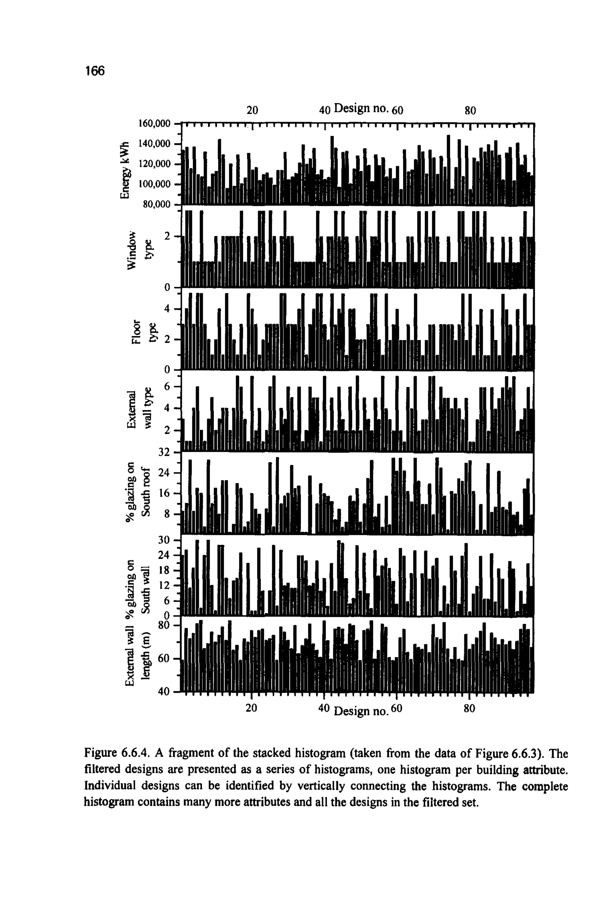
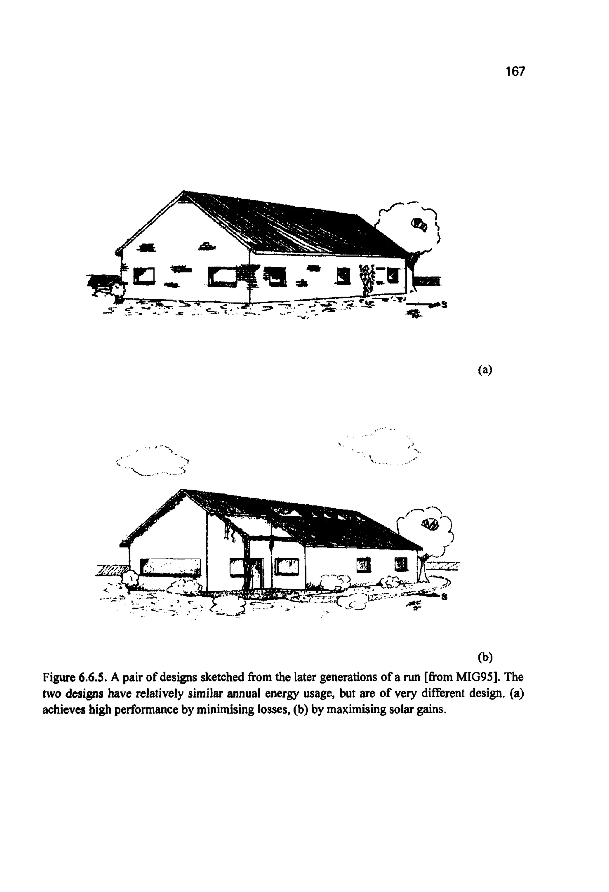
185. 168
6.7HUMANJUDGEMENTAS THEFITNESSFUNCTION
Successfulproduct design not only requires finding good engineering solutions
to the problem at hand, but often also finding aestheticallypleasing solutions to
customers' desires. The aesthetics of the solution can be extremely important
regardless of the size, or cost, of the product-from children's toys to office
blocks.
Aesthetic search spaces are typically large, complex and frequently
shaped by individual, age, gender and cultural considerations [CR84,C092b,
SH831. Often the designers' preferences will be very different from those for
whom products are being designed. The work described here (taken from
[C097a]) represents one attempt to see how successfully a genetic algorithm
could be in providing the designer with additional information. In particular,
the question of whether a GA, when applied to objects encoded in a
particularly simple manner (and driven by decisions made by a subject on the
aesthetics of a potential product), would converge at a useful rate and in the
direction of improving subject preference is addressed. Because of the many
random processes operating within the algorithm, combined with the limited
number of evaluations a human operator can be asked to perform, such an
algorithm might well perform badly.
The problem demonstrates:
0 a GA being driven by humanjudgement;
0 a problem where identical genotypes may be given non-identical values of
fitness; and
0 a system where relatively few fitness evaluationsare feasible.
COMPUTERAIDEDDESIGN
Computer aided design is becoming more common. The design environment is
typically able to present the designer with a realistic view of the item and allow
numerical analysis to be carried out to check the technical feasibility and cost
of the design. The design environment may also allow optimisation
calculations to be carried out. The optimisation itself will typically be for
maximum reliability or minimum cost [AR89].
Any aesthetic optimisation routine within such an environment would
have to contain a description of the aesthetic ideals of the target audience. This
information is often gleaned from the preferences of a market-researched
subgroup of this audience. A frequently-employed technique is to show a
number of potential designs to a series of subjects and assess the impact of the
designs upon the subjects. If these designs are actual mock-ups they will be

186. 169
very limited in number and there is the danger that one is only ascertaining the
subjects' views of what the designteam considers worthwhile;thus the subject,
and hence the potential customer, is not being truly involved in the design
process.
Computer aided design offers a way out of this trap. The computer can
offer an almost unlimited number of designs to the subject as visualisationson
the computer's screen. Such a design system can refuse to allow designs that
are unsafe, unfeasible or too costly to implement within the production
environment. However, the question remains of how the design tool and the
subjectshouldguide each otherthrough what may be a large searchspace.
THEGA DESIGNSTRATEGY
Several authors have attempted to use a GA with subjective evaluation,
including work on dam design [FU93], facial recognition [CA91] and colour
preference [HE94]. Coley and Winters [CO97a] decided to estimate the
efficacy of the GA for searchingan aesthetic, but realistic,commercialproduct
space.
It was decided to choose a realistic product in which the aesthetic
aspects of the design would be considered paramount, and one with few
engineering constraints. The chosen product was a lm square wall-hanging
containing simple geometric designs. Shapes were ascribed one of 16 basic
colours. Only isosceles triangles, rectangles, ellipses and straight lines were
considered for these basic shapes. A maximum of 20 shapes (or objects) were
present in any one design. The designs were processed by the GA as
concatenated binary strings representing the positions of comers, lengths and
the colours of the separateobjects.Although simple, the designs were realistic
and could be considered reminiscent of some of the designs contained within
paintings by CarlaPrina, Josef Albers, Piet Mondrianand Jean Gorin [SE62].
The optimisationprocess was very simple:
1.
2.
3.
4.
the computer generated an initial random population of 32 designs
together with their stringrepresentations;
the subjectviewed each designand scoredeach one for appeal;
the GA was used to produce new novel designs by crossover and
mutation of the strings;and
the process was repeated from step2 for a total of twenty generations.
Figures 6.7.l(a) to 6.7.l(f) (and the jacket cover) show a series of typical
designs.

187. 170

188. 171
Figure 6.7.I(a-f). Black and white renditions of a selectionof designsfromthe study [by
permissionftom CO97al.
The images were produced by decoding a binary string, U, of length
940 bits, consisting of a series of 20 binary substrings, ui,representing each

189. 172
object within the image. Each object itself is defined by eight parameters, pii,
which describe the type of object, its position and its colour:
U=u,@u,$u,@ ............@ u20
and
(The operator @ implies concatenation.)The precise meaning of the parameters
depend on the object in question, as described in Tables 6.7.1 and 6.7.2. For
example, the substring
UI = OIOlOI001001I000111I10000101101I000101101000011
= 01 @ 01010010@ 01100011 @ 11100001@ 01101100@ 01011010
@ 0001 @ 1.
Therefore (using Tables 6.7.1 and 6.7.2):
Thus the computer draws a visible rectangle with the above attributes as the
first object (uI).Nineteen further objects (242.....2420) are then overlaid to
complete the image.
The GA used was Goldberg's SGA [GO891 coded in C. Although the
binary search space consists of 2940(=2 ~ 1 0 ' ~ )possibilities, not all of these are
distinguishable, either because of large opaque objects covering other objects

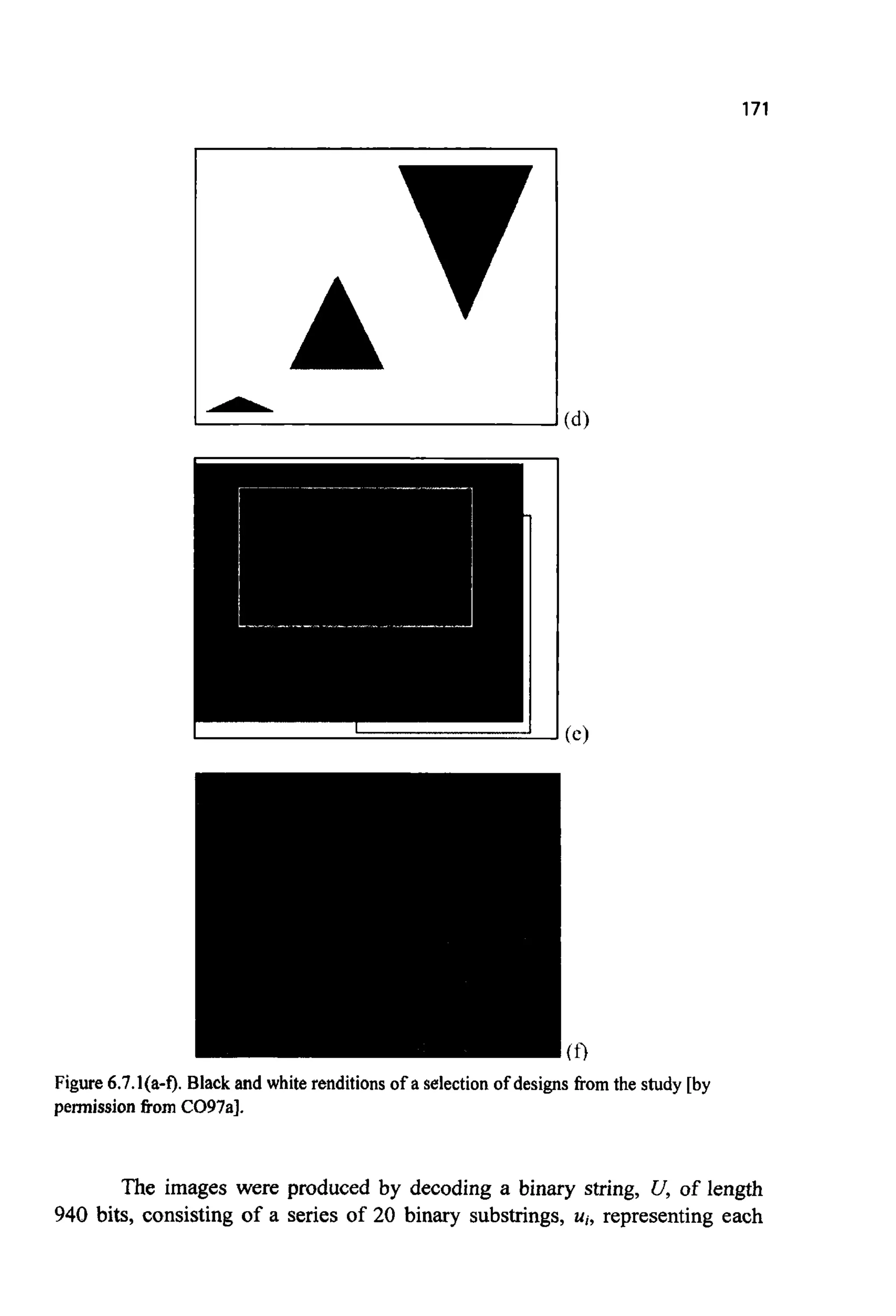
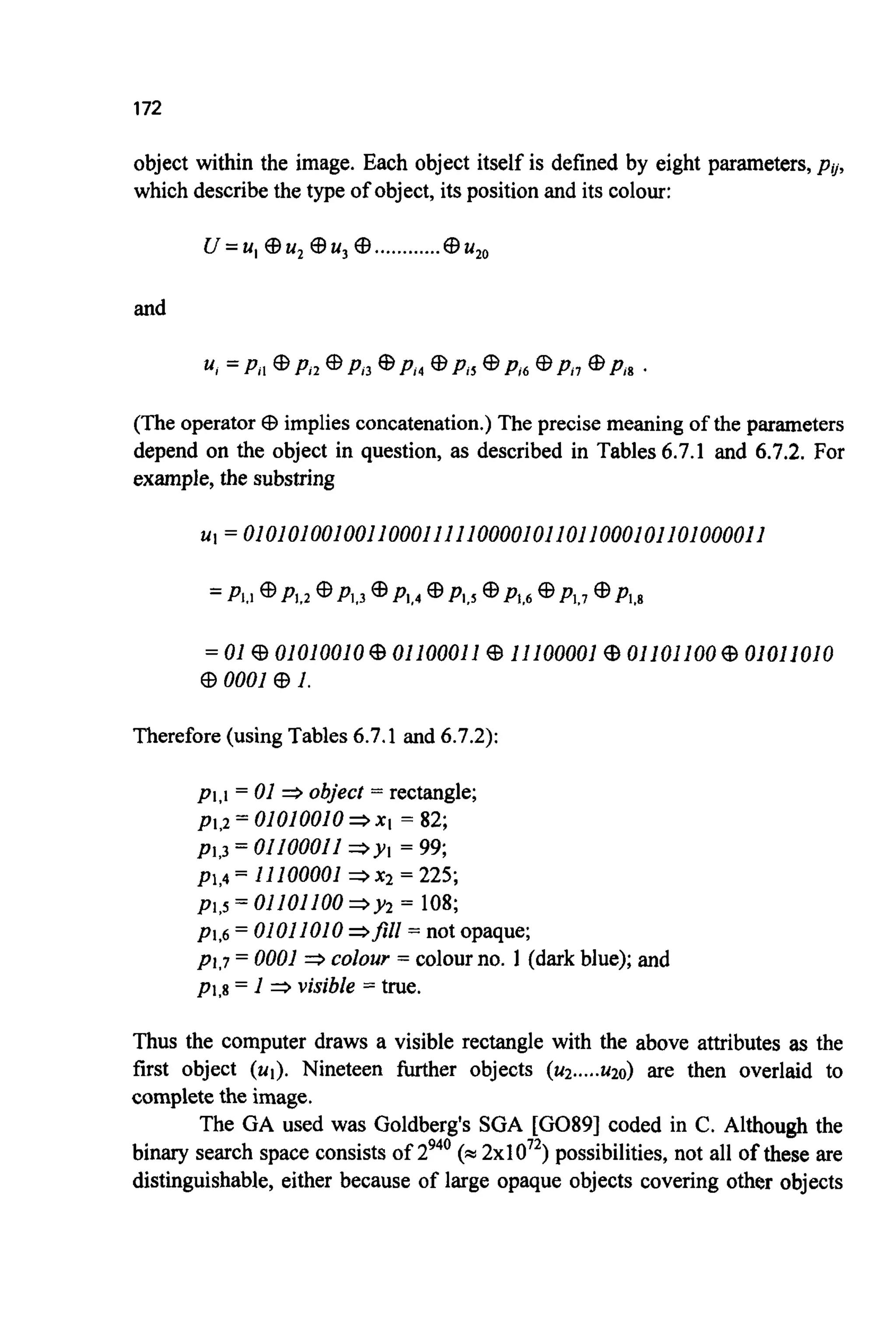
190. 173
Object
line
rectangle
ellipse
triangle
coded to the left of them on the string, or because not all combina~ionsdecode
differently(Table6.7.2).
PI Pt P3 P4 Ps P6 P7 Pa
objecttype XI YI ~2 ~2 width colour visible
objecttype XI yI x2 yz fill colour visible
objecttype XI yI r2 r2 fill colour visible
objecttype XI YI x2 height fill colour visible
Term
visible
colour
width
fill
height
-%Y1
Xl*Y2
rl+ri
type
Mkantna IntegerRmge Coding Bflr
whetherthe objectisto be drawn 0 or 1 draw if I 1
colour of the object 0 to 15 4
thickness of a straightline 0-255 INT(widW20) 8
whethera rectangleor ellipseis 0-255 opaqueif > 128 8
opaque
heightof triangle 0-255 screenco-ordinates 8
positionof the bottom left comer 0-255 screenco-ordinates 8
orcentreofellipse
position of thetop right corner 0-255 screen co-ordinates 8
lengthof major and minor axes of 0-255 screenco-ordinates 8
ellipse
whether line, rectangle,elfipse or 0-3 *tine, I=rectangle, 2
triangle 2=ellipse, 3=triangIe
Table 6.7.2. Parameterencodingsused in Table6.7.1. Trianglesalwayshave a base parallel to
the bottom of the screen. Screen co-ordinatesrun from 0 to 255 in both x- and y-directions. If
x2 <XI, or&< y ~ ,then the terms left and right,or top and bottom, reverse [CO97a].
Fitness-proportional selection was used together with single point
crossover and mutation to create new novel images. The GA is, in essence,
providing a mechanism for the melding of i ~ o ~ a t i o nwithin the images,
biased by the selection procedure toward those that receive higher scores.
However, being a stochastic algorithm, there is no guarantee that this
information will be preserved in the next generation. Mutation, for example,
couldforceradicalchangesto an image.

191. 174
SUBJECTTESTING
The design strategy was tested on 51 individuals (all undergraduates from
various University departments). The subjects were asked to score the designs
with a number between 0 and 9, the higher numbers being awarded to the
most-liked designs. The fitness function (or selection pressure) applied within
the GA was simply the score divided by 10. A crossover probability of 0.6 was
used with a mutation probability of 0.06. These parameters were chosen to
speed the search and were estimated by trial and error using additional small
groups of other subjects. Each subject viewed 20 generations of 36 images, or
720 images in total. In total the test groupviewed 36,720 images.
Figure 6.7.2 shows the score of the most-liked design (different for
each subject) as a function of generation, averaged over all subjects. The
subjects are seen to score later generations of designs higher than earlier ones.
This indicates the GA is moving towards higher scoring areas of the search
space at an observable rate. The linear overall form of the curve also indicates
that the strategy is managing to avoid becoming lost in local minima-possibly
not surprising, as so few generations are processed.
7.5 ,
% 7.0 .
c!6.5 1
2
6.0 .
j
5.5 I I I I I
0 5 10 I 5 20
Generation
7.5 -
% 7.0 -
c!6.5 1
2
6.0 -
5.5 I I I I I
0 5 10 I 5 20
Generation
Figure 6.7.2. Score of the best design as a function of generation averaged over all subjects
[CO97a].
As the scoring scale used was not absolute, it was possible that subjects
were simply ranking the later images better, regardless of content. It was also
possible, in fact likely, that they were not always consistent in their scoring.

192. 175
16
14
I2
10
8 -
6 -
4 -
2 ,
Somemight have been scoringagainst someideal design, other simply scoring
against the other images they had recently seen on the screen. An attemptwas
made to partially circumvent these problems by making use of a simple rank-
ordering method. At the end of the test, the subjects were shown a smaller
version of their most-liked design fiom each generation (simultaneously and
randomly ordered on a single screen) and asked to rank-order them.
Figure 6.7.3 shows the correlationof generation and rank-order averaged over
all the subjects.This clearly showsthat the imagescreated laterare preferred.
-
-
-
-
I I I I I
lsrt liked
i!
mort liked
Figure6.7.3. Final rank as a functionofgeneration averaged overall subjects[C097a].
One advantage of the GA is that the string representations lead
themselvesnaturally to a (simplistic)defrnitionof similarity and convergence.
By carrying out bit-wise comparisons of the strings, across all subjects, an
approximate numeric estimate of the similarity of the pictures can be made.
Without a string representation, this would have to be performed on a
qualitative visual basis by the researcher and is thus likely to be researcher-
dependent.
The results indicate that a GA-based search can be efficient in
searchingfor subjects'preferences of a real aestheticproduct. The value placed
on designs is found to rise at a usefbl rate with generation, and convergenceis
seenwithinthe bit patternsused to representthe product.However,it is not yet
clear how successful such an approach might be with other, more complex,
objects.

193. 176
6.8 MULTI-OFUECTIVENETWORKREHABILITATIONBY MESSYGA
The refurbishment of ageingwater systemsrequires decisionsto be made asto
how best to spend a limited budget in order to maximise the level of
improvement. The pre-existing network is likely to be large, complex and
costly, implying that any reasonable budget will only be able to make
alterationsto a small number of system components. This in turn implies that
most technically feasibleadjustments will not be financially feasible. Thus the
population of truly feasiblesolutionsis likely to be small in comparison to the
size of the search space. Such a search space, with most of the space counting
as unfeasible, creates problems for any optimisation routine, including a
genetic algorithm.
Godfrey Walters and Dragan Savic, working together with D. Halhal
and D. Ouazar, have formulated a structured messy genetic algorithm (SMGA)
which is p~icularlyeffectivein avoidingunfeasible parts of such a space.The
task examinedis c~mplicatedby being a mu~ti-objecti~eopti~isationprob~em
requiringtwo factorsto be simul~eously,but independently,optimised.
In the work described here, which is taken from [HA97], an SMGA is
applied to both an illustrative network and a real network of 167 pipes. The
work showsan exampleof a GA and a problem withthe followingfeatures:
0 a sparseproblem space;
0 use of a messy algorithm [Go89a];
0 a multi-objectiveproblem; and
0 fitnesssharing.
INTRODU~TION
Ageing water networks can sufferproblemsof water loss and reduced carrying
capacity. Alongside this can run increasing consumer demand. This
combination may lead to consumer discontent. However, due to budgetary and
other constraints, replacement of the complete network will be unfeasible,
unnecessary and possibly undesirable for other reasons. It is likely that funds
will only be available to replace, rehabilitate, duplicate or repair a small
number of the system components-pumps, pipes, tanks, etc.-at any one
time. Hence a decision problem arises of trying to maximise the benefits of
changes whilst remaining within a budgetary constraint. The optirnisation
problem itself is one of choosing a small number of possible designs from a
much largerset of tec~icaIlyfeasibleones.
Given a commercial operation, competition for h d s means that
designs which do not necessarily maximise benefits, but manage substantial

194. 177
improvements, may need to be considered. This implies a multiobjective
problem, where a single fitness hction cannot be formed. In this instance,the
cost of the design must be minimised, while simultaneouslythe benefit of the
design must be maximised. If an exact financial value could be placed upon all
benefits then the problem could be collapsed to a single fitness function.
However, asdiscussedin Chapter4, this is often not possible.
There have been several attempts at applying algorithmic methods to
network rehabilitationproblems [W087,KI94a,MU94]. Of particular relevance
is the work of Murphy and Simpson [MU921 who used a genetic algorithm to
find the optimal solution for a particular network. These attemptshave all been
based on small networkswith the single objectiveof minimisingcost subject to
performance constraints, such as minimum pressure for consumers. The
problem to be studied here is one of maximising benefit subject to limits on
funding.
THEPROBLEM
Given a particular, pre-existing, network the desire is to invest some or all of a
limited budget in order to enhance the performance of the network. In the
model considered,performance may be enhancedby:
1.
2.
3.
4.
increasing the hydraulic capacity of the network by cleaning, relining,
duplicatingor replacingexisting pipes;
increasing the physical integrity of the network by replacing structurally
weak pipes;
increasing system flexibilityby adding additionalpipe links; and
improvingwater qualityby removing or relining old pipes.
The problem can be stated as:
maximise Benefit(i)
minimise Cost(i)l
Cost IBudget
and
subjectto
where i representsa particularsolution.
In order to allow the GA to be able to preferentially select one solution
over another,Benefit must be able to assume a numerical value. This is done by
forminga weighted sum based on the four factors hydraulic capacity, integrity,

195. 178
flexibility and quality described above. Thus the Benefit of solution i is defined
as:
Bene$t(i) = whBh(i)+wpBp(i)+w, B, ( i ) +w,,Bq((i), (6.8.1)
where Bh, Bp,BAand By describe the hydraulic, physical, flexibility and quality
benefits respectively and Wh, wp,WJ and wgtheir respective weights (which are
user defined).
Each of the four benefits are defined as follows (for more details see
[HA97]):
0 The hydraulic benefit, Bh, is defined as the reduction of the level of
deficiency (caused by pressure shortfalls) allowed by adoption of a
particular strategy. (The nodal pressures are estimated by use of the steady-
state hydraulic network solver EPANET [ROS93].)
Improvementsto the structural condition of the network pipes reduce future
repair costs, the sum of which gives Bp.
The laying of duplicate pipes in parallel with pre-existing ones increases
the flexibility of the system, with benefit Bj, proportional to the number of
pipes replaced.
A pipe with a low Hazen-Williams (HW) factor is probably suffering from
corrosion, tuberculation or scaling-all of which can help the development
of micro-organisms or lead to discoloured water. The replacement of such
pipes can therefore lead to a water quality benefit, By,proportional to the
length of replaced pipe.
0
0
0
THESTRUCTUREDMESSYGENETICALGORITHM(SMGA)APPROACH
Messy GAS are an attempt to allow for the progressive growth in the
complexity of a solution by allowing the chromosome to increase in length
with time. This is achieved by repetitive application of a GA and the
concatenation of strings representing partial solutions. In this respect the
method imitates long-term evolution of single-cell organisms to complex life-
forms such as ourselves. It is an extremely interesting approach and allows
more traditional GASto be seen as simple adapting algorithms that in essence
fine tune the fitness of pre-existing species. With a messy GA these species
have first to be built before they are adapted to their environment. The SMGA
introducedby Halhal, Walters, Ouazar and Savic [HA971proceeds as follows:

196. 179
SteD 1 Enumerate single-variable decisions on the network-for
example, “replace pipe 89”. The point to note is that only a single decision is
being made. This implies that a great number (if not all) of such decisionsare
feasible, in that their cost will be less than the budget. This is one of the
strengthsof the approach for the type of problem considered here: right fiom
the start feasible solutions are processed. In a sparse search space, with few
feasiblesolutions,this would not be so for a more typical GA.
Because population members need to describe not only the value of a
variable but also which variable is being described, a coding scheme is
required such that an element both identifiesthe design variable and its value.
Thisfirst stage is then the enumerationof all possible single elements.
Ster,2 Filter the population to remove less well performing individuals.The
remainingindividualsare retained to provide subsequentpopulationswith high
performingelementalbuildingblocks.
SteD3 Increase the complexity of population members by adding a single
elementalbuilding block to each member (concatenation).
Step4 Use this population as the initial population of a GA and run the
algorithmuntil a terminationcriterion is met.
SteD5 Repeat from step 3, unless either the strings have reached a
predetermined length, or no improvement to the solution is seen for a set
numberof successiveconcatenationsteps.
As a stringwithinthe SMGA generally only containsa small number of
possible decision variables, its length is typically much less than that required
to contain all decision variables. This is despite the need to hold information
about the variable values as well as a tag to identifywhich variables are being
described. Not only does this improve the use of computer memory, but more
importantly, it partially circumvents the slow progress made by standard GAS
containingvery long strings.
If typically onlyp network arcs (pipes) can be considered out of a total
of q arcs because of budgetary constraints, then if each fragment can take n
alternative solutions,the search spacecontains:
(6.8.2)

197. 180
solutions [HA97]; whereas it contains
np (6.8.3)
solutions for a standard GA. If q = 60, p = 6, and n =4,then (6.8.2) implies
2 . 7 ~ 1 0 ' ~possibilities, a seemingly large space, until it is realised that (6.8.3)
implies 1. ~ x I O ~ ~possibilities.
USING THE SMGA FOR MULTIOBJECTIVEOPTIMISATION
Given more than one objective, it is impossible to form a simple fitness
function of the type used in earlier examples. One way around this would be to
use the second objective as a constraint-for example, by hunting for solutions
which provide a set minimum benefit. Another possibility would be to factor
benefits into the cost objective, by assigning benefit a financial cost. Neither of
these approaches is entirely satisfactory.
True multi-objective optimisation treats each objective separately. This
implies that each solution is not a single point in the fitness landscape, but a
vector with one dimension for each objective. The Pareto optimal set of such
vectors are those solutions which are undominated by any other solutions (see
Chapter4). For such solutions it is impossible to improve one objective
without simultaneouslymaking one or more of the other objectives worse.
It is relatively easy to use the idea of a Pareto optimal set to drive
selection within a GA. Typically, this is achieved by finding all current
members of the Pareto optimal set within the population, assigning them the
highest rank and removing them from the population-thus creating a new
Pareto optimal set (or fionr) which is assigned the next highest rank. This
process is repeated until all members of the population are ranked. Rank-order
selection is then used (together with crossover and mutation) to build the next
generation. Although simple in outline, caution is required to avoid
convergenceto a single solution.
As stressed by Halhal et al. [HA97], the SMGA is naturally suited to
multiobjectiveproblems because it ensures a good spread of different solutions
across the range of feasible costs. A standard GA is unlikely to do this because,
within a sparse solution space, many (if not most) of the members of early
generationswill represent unfeasible solutions.
For the water rehabilitation problem, the fitnessf;of each individual i
was assigned through:

198. 181
1
A=-.
FITNESSSHARING
In orderto preserve a reasone de spread of solutionsalong each Pareto optimr
front Hdh& et al. [HA971 included fitness sharing [GOS7,GO89,~E89](see
Chapter4) in the algorithm. This reduces the level of competition between
similarly ranked, but distant, population members. Niche formation and
speciation are achieved by dividing the budget into a series of intervals or
classes. Each individual is assigned to the particular interval that includes the
costof the particularsolution.
A class is deemedJirll if it contains Nin individuals, where n is the
number of classes.The shared of individuali is given by
where N&) is the number of individualsin classj. The value of n is, itself, a
functionof generation.
SMGA PARAMETERS
An integer coding is used. As discussed above, both the decision and the
decision variable must be held in the string. This is achieved by using a
substringto representall the decision variables (the arc numbers) and a second
substring to hold the decisions (what is done to each arc). For example, a
possiblestringmight be:
amsubsfring
2 1 5 3 6 1 8 2 4 2
--decision-subsfring
During the concatenationphase (step 3, above) a single digit (decision)
is added to each substringin the population. Highly performing digits from the
initid population are used unless this causes a duplicate, in which case a
r ~ d o ~digit is used. The strings (now of identical length) then undergo
processing via a conventionalGA.

199. 182
N is set to 40, with n (g= 0) set to 5. Two-point crossover is applied
separately to each substring, with child arc-substring being checked to ensure
no arcs are duplicated. Any duplications are again replaced by arcs chosen at
random.
APPLICATIONS
The SMGA was applied to the network depicted in Figure 6.8.1. The network
consists of 15 pipes, nine nodes and seven loops. There are eight possible
decisions for each pipe: “leave as is”; “clean and line”; “duplicate” (with one
of four set diameters); “renew with same diameter”; or “renew with next
largestdiameter”.The availablefund is assumed to be 2,000,000.
6
1
node
Figure 6.8.1. The test network (nodenumbers shown in italics, pipes in roman)[HA97].
The algorithm was applied with and without fitness sharing for a total
of 5,000 objective function evaluations,three times. Fitness sharing was found
to produce a slightlymore even spread of solutionsacross the range of possible
costs. The performance of SMGA (with sharing) was compared with an
integer-coded standard GA (with sharing) where the string length equalled the
number of arcs (pipes) in the network and the integer value in each string
position defined the action to be taken for the corresponding arc. The best
solutions discovered in each generation with costs less than 1.1 times the

200. 183
1400-
1200-
1000-
800 -
budget arc shown in Figure6.8.2. SMGA produced a slightly better set of
nondominated solutions. Table6.8.1 lists a selection of the nondominated
solutions(see 54.4) identified by SMGAshowing which arcs (pipes) shouldbe
replacedand which left.
o+ “1 0 : o
0
400 -
200 -
0-
-200
5
+
0 0
0
f Fund -2 million !
I . , . , .
Figure6.8.2. Best solutionsf?om each generation;+ SMGA,0 standard-GA[HA97].
Arc
80
150
80
80
80
80
80
80
80
80
80
80
Cost
1940000
1911000
1780000
1755000
1585000
1435000
138oooO
1367500
1255000
116OOOO
93oooo
750000
Arc Arc
80 150
80 150
80 150
80 150
80 80
80 150
80 150
80 100
80 80
80 150
80 150
80 80
1 2 3
Benefit I Min.
1428.96
1417.67
1414.81
1388.83
1369.52
1311.64
1305.26
1260.33
1125.96
1030.88
848.15
Pressure
&10.28
5.85
3.82
1.00
-2.47
-7.06
-15.00
-27.38
-13.54
-30.02
-60.56
L
L
L
L
Arc
15
40@
200p
L
200p
L
L
3OOp
L
L
3OOp
200p
-
2aop
Table 6.8.1. Nondominatedsolutionsfor the test network, includingnew pipe diameters(p add
parallelpipe of diametershown, L leave)[HA97].

201. 184
As a second, and more realistic, example Halhal et. al. applied the
SMGA to the network shown in Figure6.8.3 and really demonstrated the
advantages of the method. This is the water distribution of a real town of
50,000 inhabitants in Morocco. It contains 167pipes and 115 nodes. The total
number of possible solutions (assuming an unlimited string length is
6.55~10'~'.Restricting the string length to a more realistic 40 digits still
implies 8 . 6 7 ~ 1 0 ~ ~possible solutions. Halhal et. al. suggest a complete
enumeration would take 2 . 7 5 ~ 1 0 ~ ~centuries of CPU time at 1,000 objective
function evaluationsper second.
Figure 6.8.3.The real network (by permissionof ASCE [HA97]).
The benefits of the SMGA over a standard GA of fixed string length
were gauged by carrying out three independent runs of each. 25,000 objective
function evaluations were allowed in each case. The standard GA (Goldberg's
SGA [G089]) failed to converge to a design with costs less than the budget.
Even the use of a high penalty function, in order to reduce the chance of high-
cost solutions being reproduced, was only a partial improvement. It still took
7,000 objective function evaluations for the standard GA to converge to a
feasible solution. Furthermore, subpopulations in only four out of eight cost

202. 185
classeswere formed. In contrast, the SMGA formed subpopulationsin all cost
classesfiomthe b e g i ~ n g(Figure6.8.4).
240-
220 -
200-
180-
++ 4 o j
+:+ ++++ 9,
+ B
+ +
I
+ +
I40 -
120-
Cost(millions)
+ + +
+
Figure 6.8.4. Best solutionsof eachgeneration for the SMGA (+) and a standard GA (0)(data
&om [HA971).
J
loo-
80-
++
+ Fund = 2.5 million ’
I

204. 187
APPENDIXA. ELECTRONIC-AND PAPER-BASED
RESOURCES
The are many electronic- and paper-based resources available about GAS.The
internet is also an ideal way of finding those that have tried to solve similar
problems, or used similarmethods.
ELECTRONIC-BASEDRESOURCES
The following two world-wide web sites contain a multitude of information,
softwareand pointers to other GA sites:
http://alife.santafe.edu
http://www,aic.nrl.navy.mil/galist
A FORTRANGA code is availablefrom David Carroll’sweb site:
http://www.staff.uiuc.edd-carroll/ga.html
PAPER-BASEDRESOURCES
Apart from the text books mentioned at the beginning of Chapter 6, there are
several other general referenceswhich containa high density of information:in
particular, the series Foundations of Genetic Algorithms and the Proceedings
of the International Conferenceon GeneticAlgorithms:
Grefenstette,J.J, (Ed.), Proceedings of an International Conference on Genetic
Algorithms and their Applications, Morgan Kaufmann, 1985.
Grefenstette, J.J, (Ed.), Genetic Algorithms and their Applications:
Proceedings of the Second International Conference on Genetic Algorithms,
Erlbaum, 1987.
Schaffer, J.D., (Ed.), Proceedings of the Third International Conference on
GeneticAlgorithms, Morgan Kaufmann, 1989.

205. 188
Belew, R.K. and Booker, L.B., (Eds.), Proceedings of the Fourth International
Conferenceon GeneticAlgorithms, Morgan Kaufmann, 1991.
Forrest, S., (Ed.), Proceedings of the F@h Internat~onalConferenceon Genetic
Algorithms, Morgan Kaufmann, 1993.
Eshelman, L.J., (Ed,), Proceedings of the Sixth International Conference on
GeneticAlgorithms, Morgan Kaufmann, 1995.
Back, T,, (Ed,), Proceedings of the Seventh International Conference on
GeneticAlgorithms, Morgan Kaufmann, 1997.
Rawlins, G., (Ed.), Foundations of Genetic Algorithms, Morgan Kaufinann,
1991.
Whitley, D., (Ed.), Foundations of Genetic Algorifhms 2, Morgan Kauhann,
1993.
Whitley, D. and Vose, M. (Eds.), ~oundationsof Genetic Algorithms 3,
Morgan K a u f m ~ ,1995.
Belew, R.K. and Vose, M. (Eds.), Foundations of Genetic Algorithms 4,
Morgan Kaufmann, 1997.

206. APPENDIXB. A COMPLETELISTINGOF LGADOS.BAS
-- __-- _-
'LGADOS- A DOS based version of the LGA GeneticAlgorithm.
For Distributionwith the book "AnIntroductionto GeneticAlgorithmsfor
'Scientistsand Engineers",WorldScient$c 1998.
'DavidA. Coley
'ComplexSystems Group
'PhysicsBuilding
'Universiyof Exeter
'fieter
'Ex44QL
'UK
'emailD.A.Coley@exeter.ac.uk
'
I-- DECLAREALL THESUBROUTINES (PROCEDURES) USEDBY THE PROGRAM
DECLARE SUB OpenFiles ( )
DECLARE SUB Scaling (ScalingConstant!, FittestIndividual!, SumFitness!, MeanFitness!)
DECLARE SUB Elite (SumFitness!, FittestIndividual!)
DECLARE SUB Selection (mate!, SumFitness!, MeanFitness!)
DECLARE SUB Crossover (Matel!, MateZ!, NewIndividual!)
DECLARE SUB FindFitness (1
DECLARE SUB PrintGeneration (Generation, MeanFitness!, FittestIndividual!)

207. DECLARE SUB DefineRange 0
DECLARE SUB FindIntegers 0
DECLARE SUB FindUnknowns 0
DECLARE SUB Initialpopulation ( )
DECLARE SUB NoCrossover (Matel!, Matel!, NewIndividual!)
DECLARE SUB Mutate 0
DECLARE SUB Replace 0
DECLARE SUB Statistics (MeanFitness!, SumFitness!, FittestIndividual!, Generation)
'- SET ALL THEIMPORTANTFLXED PARAMETERS. -
'Theseshould be set by the user.
CONST PopulationSize = 20 'Mustbe even.
CONST NumberOfUnknowns = 2
CONST SubstringLength = 12 'Allsub-strings have the same length
CONST TotalStringLength = NumberOfUnknowns * SubstringLength
CONST MaxGeneration = 20 'G.
CONST CrossOverProbability = .6 'Pc. >=O and <=I.
CONST MutationProbability = 1 / TotalStringLength 'Pm,>=Oand<I
CONST Elitism = "ontt "'on"or "of!
CONST ScalingConstant = 1.2 'A value of 0 implies no scaling.
'-DECLARE ALL SHARED (IE. GLOBAL) VARIBLES-
The mrays that hold the individuals within the currentpopulation.
DIM SHARED Unknowns(PopulationSize, NumberOfUnknowns) AS SINGLE
DIM SHARED Integers(PopulationSize,NumberOfUnknowns) AS LONG
DIM SHARED Strings(PopulationSize,TotalStringLength)AS INTEGER
DIM SHARED Fitness(PopulationSize)AS SINGLE
The new population.

208. DIM SHARED Newstrings (PopulationSize, TotalStringLength) AS INTEGER
Themay that definesthe range of the unbmwns.
DIM SAARED Range(2, NumberOfUnknowns) AS SINGLE
The best individualin thepast generation Usedifelitism is on
DIM SHARKD Elitestring(TotalStringLength)AS INTEGER
DIM SFfARED EliteIntegers(NumberOfUnknowns)AS LO"
DIM SHARED EliteFitness AS SINGLE
DIM SHARED Eliteunknowns(NumberOfUnknowns)AS SINGLE
CLS 'Clearthe screen
ChLL Def ineRange 'Def?nethe range of eachunknown Theseshould also be set by the user.
'Setthe random numbergenerator so it produces a dferent set of numbers
'eachtime LGADOS isrum
RANWMIZE TIMER
CALL OpenFiles 'Openfiles usedto store results.
1- START OF THE GENETICALGORITHM-
1- CREATEAN INITIAL POPULATION. GENERATION 1 -
Generation = 1
Initialpopulation 'Buildapopuiation ofstrings at random
CALL FindFitness 'Findthefitnessof each member of thepopulation

209. CALL Statistics(MeanFitness, SumFitness, FittestIndividual, Generation) 'Findthe meanfitness and thefitrest -8' individual.
CALL PrintGeneration(Generation,MeanFitness, FittestIndividual) 'Printgeneration tofile.
CALL Scaling(ScalingConstant, FittestIndividual, SumFitness,MeanFitness) 'Iflinearfitnessscaling is "on"
'thenscale populationprior to selection.
I---- LOOP OVER ALL THE GENERATIONS
FOR Generation = 2 TO MaxGeneration
FOR NewIndividual = 1 TO PopulationSize STEP 2 'Loopover thepopulation choosingpairs of mates
CALL Selection(Matel,SumFitness, MeanFitness) 'Choosefirstmate.
CALL Selection(Mate2, SumFitness, MeanFitness) 'Choosesecondmate.
'Pass individuals to the temporarypopulation eitherwith or withoutperforming crossover.
IF RND c= CrossOverProbabilityTHEN 'Performcrossover.
ELSE 'Don'tperfom crossover.
END IF
CALL CrossOver(Mate1, Mate2, NewIndividual)
CALL NoCrossover(Matel,Mate2, NewIndividual) 'Dont'tperform crossover.
NEXT NewIndividual
CALL Mutate 'Mutatethe temporarypopulation.
CALL Replace 'Replacethe oldpopulation completelyby the new one.

210. CALL FindUnknowns 'De-codethe newpopulaton to integersthenred numbers.
CALL FindFitness 'Findthefrh2ess of eachmember of thepplatiom
CALL Statistics(MeanFitness,SumFitness, FittestIndividual, Generation) 'Findthemeanfitnessandthe Pttest
individual.
CALL PrintGeneration(Generation,MeanFitness, FittestIndividual) 'Printgenerationtofile.
CALL Scaling(ScalingConstant, FittestIndividual, SumFitness, MeanFitness) 'Ifhzearfitness scaling is "on"
* thenscalepopulationprior toselection.
NEXT Generation 'Processthenextgeneration.
CLOSE 'Closeallfiles
SUB Crossover (Matel,Mate2, NewIndividual)
'Pe$orm singlepoint crossover.
Crosssite = I"I?( (TotalStringLength- 1) RND + 1) 'Pickthe cross-site at random
FOR Bit = 1 TO Crosssite 'Swapbits to the lefi of the cross-site.
NewStrings(NewIndividua1, Bit) = Strings(Mate1, Bit)
NewStrings(NewIndividua1 + 1, Bit) = Strings(Mate2, Bit)
NEXT Bit
FOR Bit = Crosssite + 1 TO TotalStringLength 'Swapbits to the right of the cross-site.
Newstrings (NewIndividual,Bit) = Strings(Mate2, Bit)
Newstrings (NewIndividual+ 1, Bit) = Strings(Matel,Bit)
NEXT Bit

211. END SUB
SUB DefineRange
'Definesthe upper and lower bouna!sof each unknown.
'Addother ranges using thesameformat ifmore than two unknownsin theproblem.
unknown = 1 'thefirstunknown.
Range (1, Unknown) = 0 'Thelowerbound
Range(2, Unknown) = 1 'Theupperbound
unknown = 2 'thesecondunknown
Range(1, Unknown) = -3.14159
Range(2, Unknown) = 3.14159
'Addother ranges ifmore than two unknownsinyour problem.
END SUB
SUB Elite (SumFitness, FittestIndividual)
'Applieselitbm by replacinga randomlychosenindividual
pom thepreviouspopulationifthe new mmfitness is less then theprevious value.
IF Fitness(FittestIndividua1) < EliteFitness THEN
the elitemember
Individual = 1"T (PopulationSize RND + 1) 'Chosenindividualto be replaced
FOR Bit = 1 TO TotalStringLength
Strings(Individua1, Bit) = EliteString(Bit1
NEXT Bit

212. Fitness(Individua1) = EliteFitness
FOR Unknown = 1 TO NumberOfUnknowns
Integers(Individua1, Unknown) = EliteIntegers(Unkn0wn)
Unknowns(Individua1, Unknown) = EliteUnknowns(Unknown)
NEXT Unknown
FittestIndividual = Individual
END IF
FOR Bit = 1 TO TotalStrinqLength
NEXT Bit
EliteStrinq(Bit) = Strings(FittestIndividua1, Bit)
EliteFitness = Fitness(FittestIndividua1)
FOR Unknown = 1 TO NumberOfUnknowns
EliteInteqers(Unknown) = Integers(FittestIndividua1, Unknown)
EliteUnknowns(Unkn0wn) = Unknowns(FittestIndividua1, Unknown)
NEXT Unknown
END SUB
SUB FindFitness
‘Theproblem at hand is used to assign apositive (orzero)fitness to each individual in turn.
‘Theproblem isf =x”2 +sin&).
FOR Individual = 1 TO PopulationSize
Fitness (Individual) = Unknowns (Individual, 1) * 2 + SIN (Unknowns(Individual, 2) )
If Fitness(Individua1) c 0 then Fitness(Individua1) = 0

213. NEXT Individual
END SUB
SUB FindIntegers
'Decode the strings to sets of decimal integers.
DIM bit AS INTEGER
FOR Individual = 1 TO populationsize
bit = TotalStringLength + 1
FOR Unknown = NumberOfUnknowns TO 1 STEP -1
Integers (Individual, Unknown) = 0
FOR StringBit = 1 TO SubstringLength
bit = bit - 1
IF Strings(Individua1, bit) = 1 THEN
END IF
Integers (Individual, Unknown) = Integers(Individual, Unknown) + 2 * (StringBit - 1)
NEXT StringBit
NEXT Unknown
NEXT Individual
END SUB
SUB Findunknowns
'Decode the strings to real numbers.
CALL FindIntegers 'Firstdecode the strings to sets of decimal integers.
'Now convert these integersto re&.
FOR Individual = 1 TO Populationsize

214. FOR Unknown = 1 TO NumberOfUnknOWnS
UnJcnowns (Individual, Unknown) = Range(1, Unknown) + Integers(Individual,Unknown) * (Range( 2 ,
Unknown) - Range(1, Unknown)) / ( 2 A SubstringLength - 1)
NEXT Unknown
NEXT Individual
END SUB
SUB Initialpopulation
‘Createthe initialrandompopulation
FOR Individual = 1 TO PopulationSize
FOR Bit = 1 TO TotalStringLength
Strings (Individual,Bit) = 1
Strings (Individual,Bit) = 0
IF RND .5 THEN
ELSE
END IF
NEXT Bit
NEXT Individual
CAU FindUnknowns ‘Decodestringsto real numbers.
END SUB
SUB Mutate
’Visit eachbit of eachstringvery occasionallyjlippinga “1” to a ”0”or viceversa
FOR Individual = 1 M PopulationSize

215. FOR Bit = 1 TO TotalStringLength
'Throwa random number andsee ifit isless than or equal to the mutationprobabiliv.
IF RND c= MutationProbability THEN
'Mutate.
IF NewStrings(Individua1, Bit) = 1 THEN
Newstrings (Individual, Bit) = 0
ELSE
Newstrings (Individual, Bit) = 1
END IF
END IF
NEXT Bit
NEXT Individual
END SUB
SUB Nocrossover (Matel, Mate2, NewIndividual)
'Passthe selected strings to the temporqpopulation withoutapplying crossover.
FOR Bit = 1 TO TotalStringLength
NewStrings(NewIndividua1, Bit) = Strings(Mate1, Bit)
Newstrings (NewIndividual + 1, Bit) = Strings(MateZ, Bit)
NEXT Bit
END SUB
SUB OpenFiles

216. '+en resnltflts.See Chqvter2fwahuiption of theircant-.
OPEN *LoADoS.RES" FOR APPEND AS #1
OPEN "LoAwS.ALL" FOR OUTPUT AS #2
END SUB
SUB PrintGeneration (Generation, MeanFitness, FittestIndividual)
'Printresults to thescreen and tkfi1e.x
PRINT Generation; Fitness(FittestIndividua1); MeanFitness; 'screen
PRINT #1, Generation; I,";Fitness(FittestIndividual); I ,";MeanFitness; 'FileLGADOS..REs.
FOR Unknown = 1 TO NumberOfUnknowns
PRINT Unknowns (FittestIndividual,Unknown); screen
PRINT #1, ,It; unknowns (FittestIndividual,Unknown); 'FileL G A D 0 S . D
NEXT Unknown
PRINT 'Carriagereturn
PRINT #1, 'carriage return
FOR Individual = 1 TO populationsize
PRINT #2, Generation; 'I, ; Fitness(Individual); I t , 'I ; 'FileLGADOSALL
FOR Unknown = 1 TO NumberOfUnknOwnS
PRINT # 2 , unknowns(Individual, Unknown); ", ; 'FileLGAD0S.m
NEXT Unknown
FOR Bit = 1 TO TotalStringLength

217. PRINT #2, RIGHT$ (STR$(Strings(Individual, Bit)) , 1) ;" ,'I ; 'FileLGALK)SALL
NEXT Bit
PRINT # 2 , 'Carriagereturn
NEXT Individual
END SUB
SUB Replace
'Replacefheoldpopulation with the new one.
FOR Individual = 1 TO PopulationSize
FOR Bit = 1 TO TotalStringLength
NEXT Bit
Strings(Individua1, Bit) = NewStrings(Individua1, Bit)
NEXT Individual
ERASE Newstrings 'Clearthe old array ofstrings.
END SUB
SUB Scaling (ScalingConstant, FittestIndividual, SumFitness, MeanFitness)
'ApplyLinear Fitness Scaling,
' scaledfimess = a *fitness + b.
'Subjectto,
' meanscaledfimess= meanfimess
'and
'
khere c, the scaling constant,is set by the user.
bestscale&tness = c *rneanfimess,

218. 'rfthescalingconstmrtissetto zero, or all individuals have thesamefimes, scaling isnot qpIied
IF ScalingConstant c> 0 AND Fitness(FittestIndividua1) - MeanFitness > 0 TIIEN
'Findaandb.
a = (ScalingConstant- 1) MeanFitness / (Fitness(FittestIndividua1)- MeanFitness)
b = (1 - a) MeanFitness
'Aajustthefmas of all members ofthepopulation.
SumFitness = 0
FOR Individual = 1 TO PopulationSize
Fitness(Individual) = a Fitness(Individual)+ b
IF Fitness (Individual)c 0 THEN Fitness(Individual) = 0 'Avoidnegativevdues near the endof a run.
SumFitness = SumFitness + Fitness(Individual)'Ad/ustthe sum of allthejimessa.
NEXT Individual
'AGustthe mean of all thefimasa.
MeanFitness = SumFitness / PopulationSize
END IF
END SUB
SUB Selection (mate, SumFitness, MeanFitness)
'Selecta single individualbyfitnessproportionalselection.
Sum = 0
Individual = 0
Roulettemeel = RND * SumFitness

219. Do
Individual = Individual + 1
Sum = Sum + Fitness(Individua1)
LOOP UNTIL Sum >= Roulettewheel OR Individual = PopulationSize
mate = Individual
END SUB
SUB Statistics (MeanFitness, SumFitness, FittestIndividual, Generation)
'Cddatethesum offitnew acrossthepopdation andfind the best individual
'thenppty elitismifrequired
FittestIndividual = 0
MaxFitness = 0
FOR Individual = 1 TO PopulationSize
MaxFitness = Fitness(Individua1)
FittestIndividual = Individual
IF Fitness(Individua1) > -Fitness THEN
END IF
NEXT Individual
IF Elitism = "on" "'HEN 'Appbelitism.
END IF
CALL Elite(SumFitness, FittestIndividual)
SumFitness = o 'Sumthefimess.
FOR Individual = 1 TO PopulationSize
NEXT Individual
SumFitness = SumFitness + Fitness(Individua1)

220. 203

222. 205
REFERENCES
AL77
At95
AN89
AR89
BAS5
BA91
BA93
BA96
BE93
BE93a
Alperovits, E and Shamir,U,Design of optimal water d i s ~ ~ ~ u t i o nsystems, Water
Resour. Res. 13(6), p885-900, 1977.
Altenberg, L., The schematheorem and Price's theorem, Whitley, L.D. and Vose,
M., (Eds.), Foundatom of GeneticAlgorjthms3,Morgan Kaufmann, 1993.
Antonisse, J., A new interpretationof schema notation that overturns the binary
encoding constraint, in Schaffer, J.D.,(Ed.), Proceedings of the 3d International
Conferenceon GeneticAlgorithms,Morgan Kaufmann, p86-91, 1989.
Arora, J.S.,Introductionto Optimum Designs,McGraw-Hill, 1989.
Baker, J.E., Adaptiveselectionmethods for genetic a l g o ~ ~ ~ s ,proceeding^ of an
~nternationalconferenceon GeneticAlg5rithmsand theirApplicat~o~,p101-1I 1,
1985.
Baker, J. E., Reducingbias and inefficiencyin the selection algorithm, in Genetic
Algorithms and their Applications: Proceedings of the Second International
Conferenceon GeneticAlgorithms, 1987.
Back, T., Hofbeister, F. and Schwefell, H., A survey of evolution strategies, in
Belew, R.K. and Booker, L.B., (Eds), Proceedings of fhe 4" International
Conferenceon GeneticAlgorithms,Morgan Kaufmann, p2-9,1991.
Back, T., Optimal mu~tionrates in genetic search, in Genetic AJgorifhms:
Proceedingsof fhe 5Ih~n~ernaf~onalConzrence, Forrest, S.,(Ed.), p2-8, Morgan
Kaufmann, 1993.
Bbck, T., Evolutionary Algorithms in Theory and Practice, Oxford University
Press, New York, 1996.
Bertoni, A. and Dorigo, M., Implicit parallelism in genetic algorithms, Artificial
Intelligence,61(2), p307-314, 1993.
Beasley, D.,Bull. D.R.and Martin, R.R., A sequentiai niche technique for

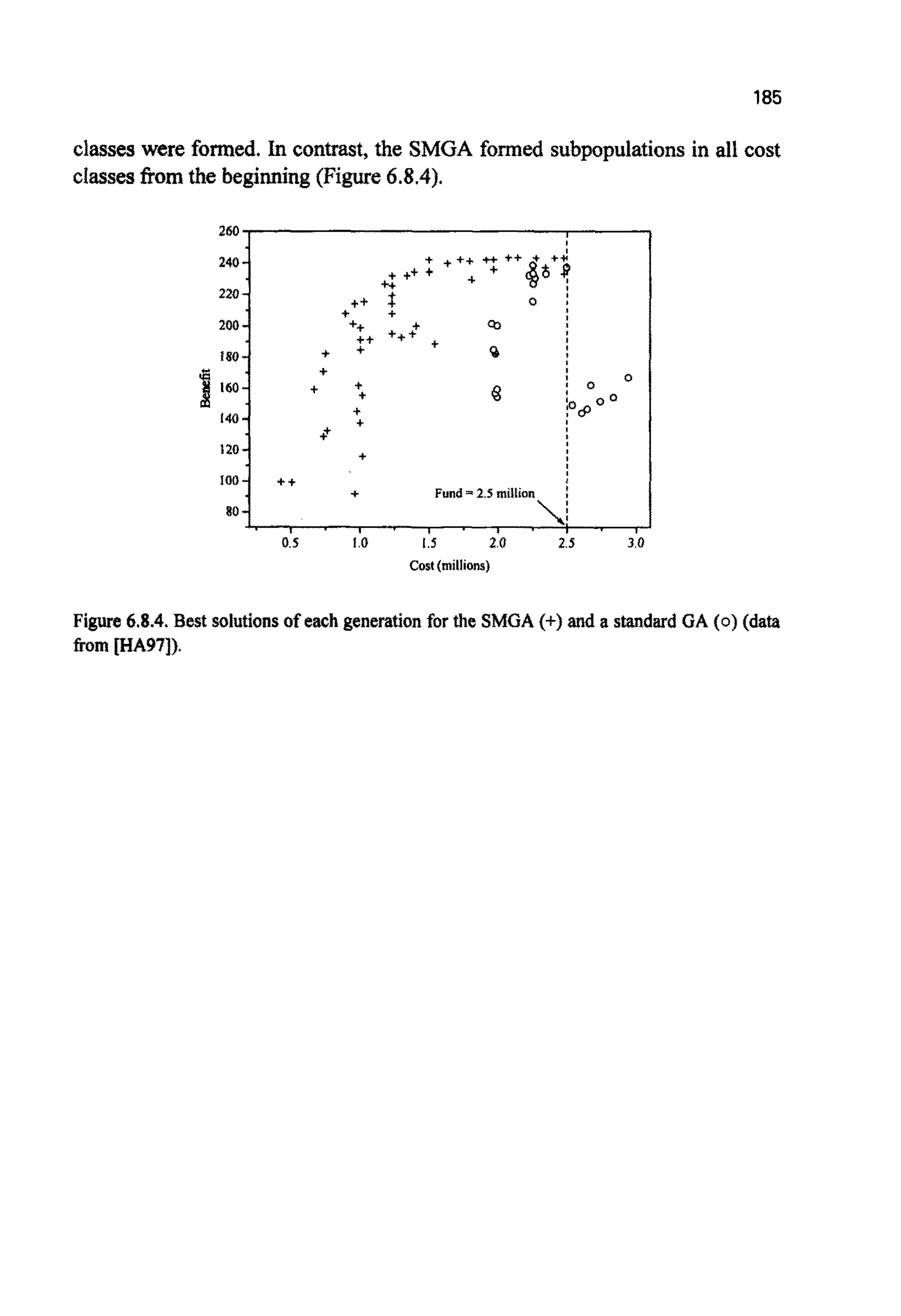
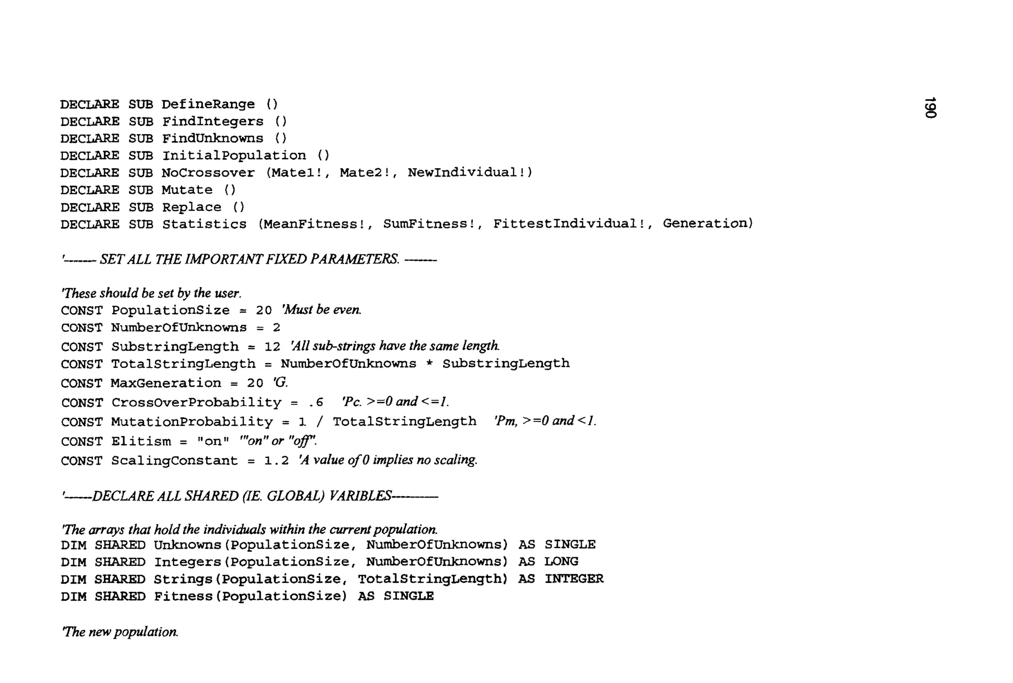
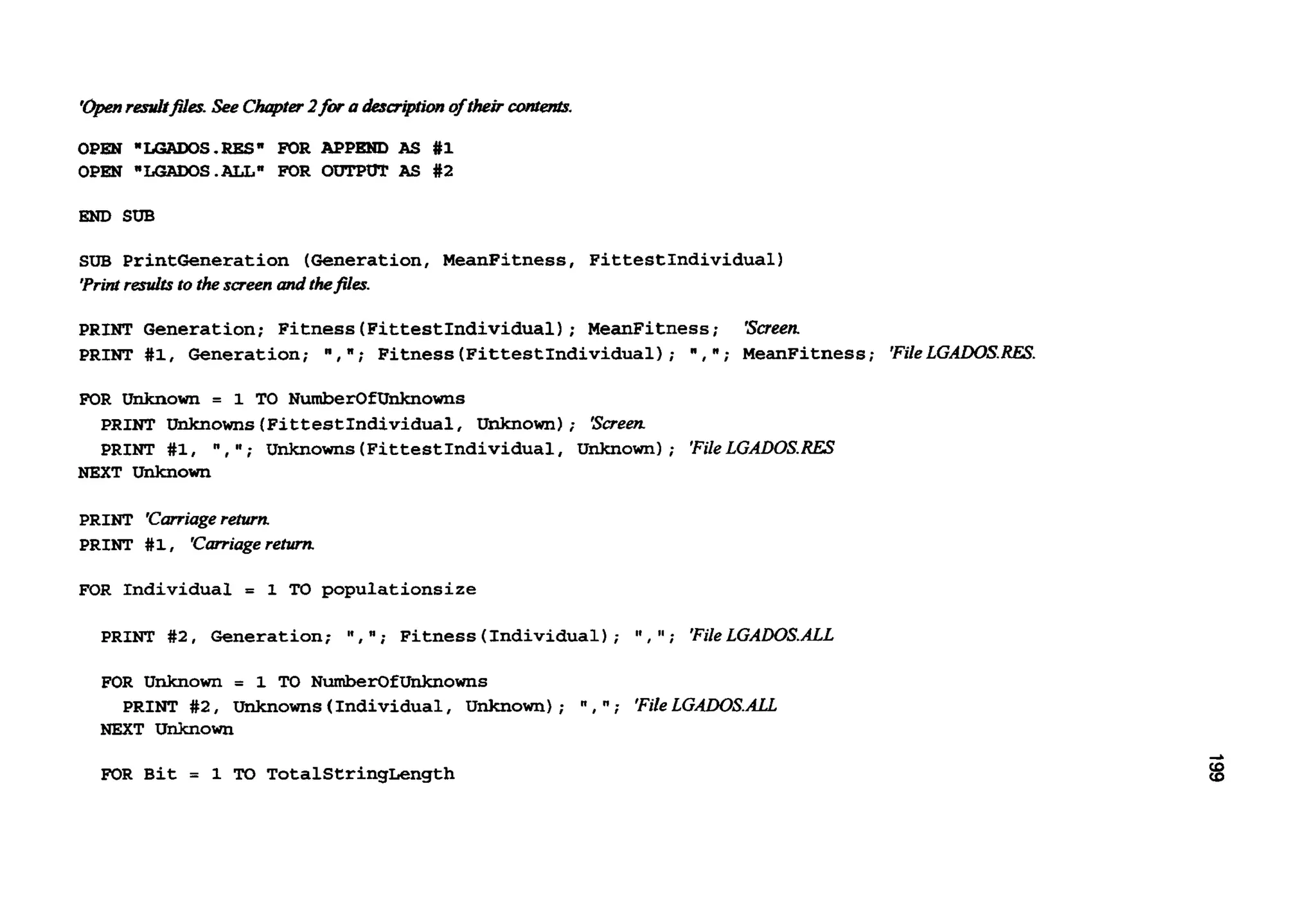
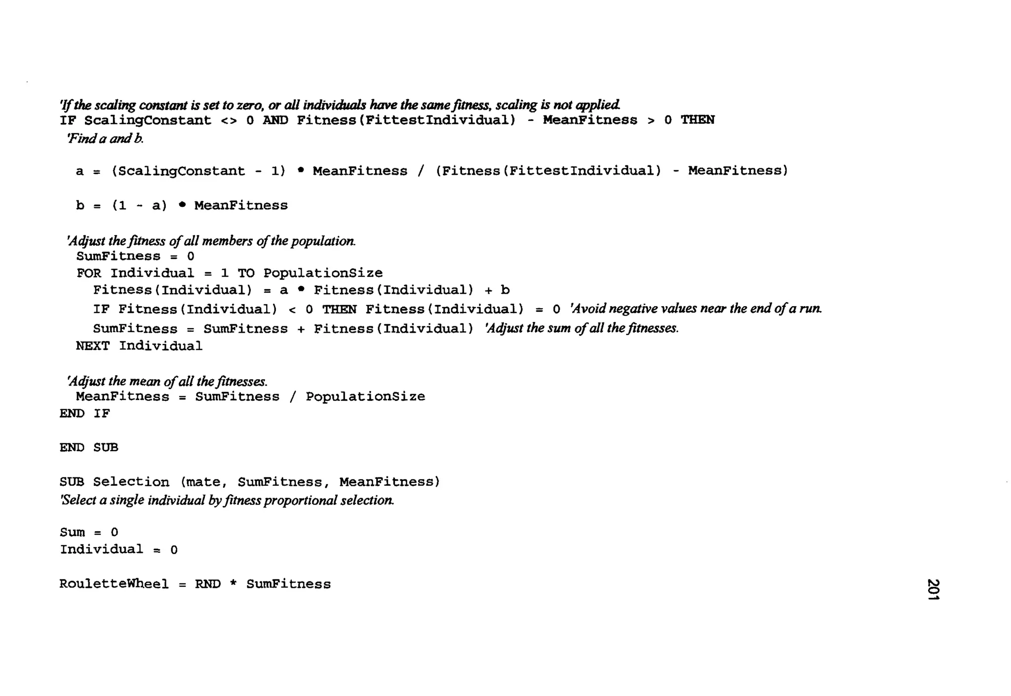
223. 206
B186
BL95
9087
BR89
BR9I
BU84
CA89
CA91
CA96a
CA96b
multimodal hction optimization, Evolutionary Computation, 1(2), p101-125,
1993.
Binder,K.and Young,A.R., Rev. Mod Phys. 58,p801, 1986.
Blickle, T. and Thiele, L., A mathematical analysis of tournament selection, in
Eshelman, L.J., Proceedings of the dh International Conference on Genetic
Algorithms,p506-511, 1995.
Booker, L., Improvingsearchin geneticalgorithms,in [DA87], p61-73, 1987.
Bramlette, M.F.and Cusic, R., A comparative evaluation of search methods
applied to the parametric design of aircraft, Schaffer, J.D., (Ed.), Proceedings of
ihe 3"' ~niernationalConferenceonGenetic~lgorifhms,M o r ~Kau~ann,1989.
Bramlette, M.F.,Initialization, mutation and selection methods in genetic
algorithms for function optimisation, in Belew, R.K. and Booker, L.B., (as),
Proceedings of the 4" International Conference on Genetic Algorithms,Morgan
Kaufmann, 1991.
Bunday, B.D., Basic Optimisa#ionMethoak,EdwardArnold, London, 1984.
Caruana, R.A., Eshelman, L.J. and Schaffer,J.D., Representationand hidden bias
11: estimating defining length bias in genetic search via shuMe crossover, in
Proceedings of the I I" i~erna~ionaIJoint Confirence on ~ r t ~ c ~ a irn~eIl~gence,
Morgan Kaufmann, San Mateo,p750-755,1989.
Caldwell, C. and Johnston, V.S.,Tracking a Criminal Suspect Through "Face-
Space" with a Genetic Algorithm, in Belew, R.K. and Booker, L.B., (Eds),
Proceedings of the 6-kZnternationaZ Confirence on GeneticAigor~fh~s,Morgan
K a u ~ a ~ ,p416-421,1991.
Carroll, D.L., Chemical Laser Modelingwith Genetic Algorithms,AIAA Journal,.
34(2), pp. 338-346, February 1996.
Carroll, D.L., Genetic A l g o r i ~ sand Optimizing Chemical Oxygen-Iod~e
Lasers, Developments in Theoretical and A ~ p ~ ~ e dMechanics, Vol. XVKII, eds.
Wilson, H.B., Batra, R.C., Bert, C.W., Davis, A.M.J., Schapery, R.A., Stewart,
D.S. and Swinson, F.F., School of Engineering, The University of Alabama, ,

224. 207
pp.411-424, 1996.
CE93
CH90
CH96
CH97
C092
C092a
C092b
C094
C094a
C096
C097
Celik, T., Hausmann U.H.E. and Berg B., Computer Simulation Studies in
Condensed Matter VI, Landau, D.P., Mon, K.K., and Schuttler, H.B., (Eds.),
SpringerVerlag, Heidelberg,p173, 1993.
Chalmers, D.J., The evolution of learning: an experiment in genetic
connectionism, in Touretzky, D.S., Elman, J.L., Sejnowski, T.J. and Hinton, G.E.,
(Eds.), Proceedings of the 1990 ConnectionistModels Summer School, Morgan
Kaufmann, 1990.
Chipperfield, A. and Fleming, P., Genetic algorithms in control systems
engineering,J. of Computersand Control,24(I), 1996.
Chen, Y.W.,Nakao, Z., Arakaki, K., Tamura, S., Blind deconvolution based on
genetic algorithms, IEICE Transactions on Fundamentals of Electronics,
Communicationsand ComputerSciences,E80A(12), p2603-2607, 1997.
Coley, D.A. and Penman, J.M., Second order system identification in the thermal
response of a working school: Paper 11. Building and Environment 27(3) 269-277,
1992.
Collins, R.J. and Jefferson, D.R., The evolution of sexual selection and female
choice, Varela, F. J., Bourgine, P., (Eds.), Toward a Practice of Autonomous
Systems: Proceedings of the First European Conference on Artificial Lfe, MIT
Press, 1992.
Cooper, D.E. (Ed.), A Companionto Aesthetics,Blackwell, 1992.
Coley, D.A. and Bunting, U., The identification of complex objects from NMR
Imagesby GeneticAlgorithm,IEE Digest 193p91-96, 1994.
Coley, D.A. and Crabb, J.A.. ComputerisedControl of artificial light for maximum
use of daylight, LightingRes. Technol.26 (4) p189-194, 1994.
Coley, D.A., Genetic Algorithms, C0ntemporar)iPhysics,37(2) p145-154, 1996.
Coley, D.A. and Crabb, J.A., An artificial intelligenceapproachto theprediction
of naturallightinglevels,Building and Environment, 32(4), p81-85, 1997.

225. 208
C097a
COH91
CR84
CR87
CR87a
DA87
DA89
DA91
DA91a
DA91b
Coley, D.A. and Winters, D., Search Eflcaq in Aesrhetic Product Spaces,
Complexity, 3(2), p23-27, 1997.
Cohoon, J.P., Hegde, S.U.,Martin, W.N. and Richards, D.S., Distributed genetic
algorithms for the floorplan design problem, IEEE Trans., CAD, 10(4), p483-492,
1991.
Crozier, R.W. and Chapman, A.J. (Eds.), Cognitive Processes in the Perception of
Art, North-Holland, 1984.
Crabb, J.A., Murdoch, N. and Penman, J.M., Validation study of EXCALIBUR, a
simpli~edthermal response model, BujfdingServices Research and TechnorogY 8
p13-19, 1987.
Crabb, J.A., Murdoch, N. and Penman, J.M., Building energy assessment by
simplified dynamic simulation model, presented at the European Conference on
Architecture, Munich, April 1987.
Davis, L. (Ed.), Genetic algorithms and simulated annealing, Pitman, London,
1987.
Davis, L., Adapting operator p~babilitiesin genetic algorithms, in Schaffer, J.D.,
(Ed.), P~oceedjngsof the 3& in~erna~ion~lConference on Genetic Algorithms,
Morgan Kautinann, p61-69, 1989.
Davis, L., (Ed.), Handbook of Genetic Algorithms, Van Nostrand Reinhold, New
York, 1991.
Davidor, Y.,A naturally occurring niche and species phenomenon: the model and
first results, in Belew, R.K. and Booker, L.B., (Eds), Proceedings of the #Ih
international Conferenceon Genetic Algorithms, Morgan Kaufmann, p257-263,
1991.
Davis, L., Bit-climbing, represen~ationalbias and test suit design, in Belew, R.K.
and Booker, L.B., (Eds), Proceedings of the 6 Internationai Conference on
GeneticAlgorithms,Morgan Kaufmann, pl8-23, 1991.
DE75 De Jong, K.A., Analysis of the behaviour of a class of genetic adaptive systems,

226. 209
DE89
DE89a
DE93
DE93a
DO91
DU90
ED75
EE9I
EE94
EI94
EL85
Doctoral dissertation, University of Michigan, DissertationAbstracts International
36(10), Si40B,university Micro~ImsNo. 76-9381), 1975.
Deb, K., GeneticA~go~ifh~sin m ~ l t j - m o ~ ~ ~ n c ~ i o n# ~ ~ ~ r n ~ a f ~ o n ,Mastersthesis,
The Centre for Genetic Algorithms Report No. 89002, University of Alabama,
1989.
Deb, K., and Goldberg, D.E., An investigationof niche and species formation in
genetic function optimisation, in Schaffer, J.D., (Ed.), Proceedings of the 3&
Znferna~i~a~Con~erenceon GeneticA~gor~ghms,MorganKaufma~,1989.
De Jong, K,A., GeneticalgorithmsareNOTfunctionoptimisers,In Whitley, L.D.,
(Ed.), Fou~at~onrofGeneticAlgorithms2, MorganKaufinann, 1993.
De Jong, K, A. and Sarma, J., ene era ti on gaps revisited, ~ i t l e y ,L.D., {Ed.),
Foundationr ofGeneticAlgorithms2, Morgan Kaufmann, 1993.
Dodd, N., Mac~~ane,D., and Marland, C.,Optimisation of artificia1 neural
network structure using genetic techniques imp~eme~edon multiple transputers,
Transparing '91,Vol. 2,IOS Press, p687-700, 1991
Duan, N.,Mays, L.W. and Lansey, K.E., Optimal reliability-based design of
pumpingand distributionsystems,J. My&. Engrg.,ASCE, IlqZ), 249-268,1990.
Edwards,S.F. and Anderson, P. W., J. Phys. F,5,965,1975.
Energy EBciency in Oflccas:A TechnicalGuidefor Owners and Single Tenants,
EnergyConsumptionGuide 19.UK Energy Efficiency Office, 1991.
&rduct/on to Energy Eflciency in Schools, Department of the Environment
Energy EmciencyOffice, 1994.
Eiger, G,,Shamir, U. and Ben-Tal, A,, Optimal design of water distribution
networks, Water Resow.Reg.,30(9), p2637-2646,1994.
EI-Bahrawy, A. and Smith,A.A., Application of MINOS to water collection and
dis~ibutionnetworks,Civ.Engrg Sys., 2(1), ~3849,1985.
ES89 Eshelman, L.J., Caruana, R.A. and Schaffer, J.D., Biases in the crossover

227. 210
landscape, in [SC89, p10-19], 1989.
ES91
ES91a
ES93
ES94
FA94
FE88
F184
F066
F089
F093
FON93
Eshelman, L.J., The CHC adaptive search algorithm: how to have safe search
when engaging in non-traditional genetic recombination, Rawlins, G., (Ed.),
Foundationsof GeneticAlgorithms,Morgan Kaufmann, 1991,
Eshelman, L.J. and Schaffer, J.D., Preventing premature convergence in genetic
algorithms by preventing incest, in Belew, R.K. and Booker, L.B., (Eds),
Proceedings of the 4" International Conferenceon Genetic Algorithms, Morgan
Kaufmann, 1991.
Eshelman, L.J. and Schaffer, J.D., Real-coded algorithms and interval-schemata,
Whitley, D. (Ed.), Foundationsof GeneticAlgorithms 2, Morgan Kaufmann, 1993.
Esbensen, H. and Mazumder, P., SAGA: a unification of the genetic algorithm
with simulated annealing and its application to macro-cell placement, Proceedings
of the 7Ih Int. Conj on VLSIdesign, p211-214, 1994.
Fausett, L., Fundamenfalsof neural nehvorks,Prentice-Hall International, 1994.
Feder, J.. Fractals, Plenum Press, New York, 1988.
Fitzpatrick J.M., Grefenstette J.J. and Van Gucht D. Image registration by genetic
search, Proceedingsof IEEE Southeast Conferencep460-464, 1984.
Fogel, L.J., Owens, A.J. and Walsh, M.J., Artificial intelligence throughsimulated
evolution,Wiley, New York, 1966.
Fogarty, T.C., Varying the probability of mutation in the genetic algorithm, in
Schaffer, J.D., (Ed.), Proceedings of the 3" International Conference on Genetic
Algorifhms,Morgan Kaufmann, plO4-109, 1989.
Forrest, S.and Mitchell, M., relative building block fitness and the building block
hypothesis, In Whitley, L. D., (Ed.), Foundationsof GeneticAlgorithms 2, Morgan
Kaufmann, 1993.
Fonseca, C.M. and Fleming, P.J., Genetic algorithms for multiobjective
optimisation: formulation, discussion and generalisation, in Genetic Algorithms:
Proceedings of the 5" International Conference, Forrest, S., (Ed.), p416-423,

228. 211
Morgan Kaufmann, 1993.
FU90
FU93
FUR0
GE85
GO87
G087a
GO89
G089a
G089b
GO91
GO91a
Futuyma, D.J., fivolutionsbiologie,Birkhtiuser Verlag, Basel, 1990.
Furuta, H. et. al., Applicationof the genetic algorithm to aesthetic design of dam
structures,Proceedings Neural Networks and CombinatorialOptimization in Civil
and Strucrural Engineering Conference, Edinburgh (1993), published by Civil
Comp Ltd,p101-109, 1993.
Fujiwara, 0. and Khang, D.B., A two-phase decomposition method for optimal
design of looped water distribution networks, Water Resour. Res., 26(4), p539-
549,1990.
Gessler, J., Pipe network optimization by enumeration, Proc. Spec. Con$ on
Comp.Applications/WaterResour.,ASCE, New York, p572-581, 1985.
Goldberg, D.E., and Richardson, J., Genetic algorithms with sharing for
multimodal function optimisation, Genetic algorithms and their applications:
Proceedings of the r"'International Conference on Genetic Algorithms, p41-49,
1987.
Goldberg, D.E. and Kuo, C.H.,Genetic algorithms in pipeline optimization, J.
Comp.in Civ.Engrg.,1(2), p128-141, 1987.
Goldberg, D.A., Genetic Algorithms in Search, Optimisation and Machine
Learning,Addison-Wesley, 1989.
Goldberg, D.E., Korb, B., and Deb, K., Messy genetic algorithms: Motivation,
analysis,and first results.ComplexSystems,3(4),p493-530, 1989.
Goldberg, D.E., Sizing populations for serial and parallel genetic algorithms, in
Schaffer, J.D., (Ed.), Proceedings of the 3" InternationalConfrence on Genetic
Algorithms,Morgan Kaufmann, p70-79, 1989.
Goldberg, D.E. and Deb, K., A comparativeanalysis of selection schemes used in
genetic algorithms, Rawlins, G., (Ed.), Foundations of Genetic Algorithms,
Morgan Kaufmann, p69-93, 1991.
Goldberg, D.E. and Deb, K. and Bradley, K., Don't worry,be messy, in Belew,

229. 212
GO93
GOT89
GOU86
GR85
GR86
GR89
GR91
GR93a
GR97
HA88
R.K. and Booker, L.B., (Eds), Proceedings of the 4" International Conferenceon
GeneticAlgorithms,Morgan Kauhann, p25-30, 1991.
Goldberg,D.E., Deb, K., Kargupta, H. and Harik, G., Rapid, accurateoptimization
of difficult problems using fast messy genetic algorithms, in Genetic Algorithms:
Procee~ingsof the Sfh lnternaiiona~Conference, Forrest, S., (Ed.), p56-64,
Morgan Kaufinann, 1993.
Gottschalk, W., Allgemeine Genetik,Georg Thieme Verlag, Stuttgart, 3"' edition,
1989.
Goulter, I.C., Lussier, B.M.and Morgan, D.R., Implications of head loss path
choice in the optimisation of water distribution networks, Water Resour. Rex,
22(5), ~819-822,1986.
Grefenstette, J.J., Gopal, R., Rosmaita, B.J., and Van Gucht, D., Genetic
algorithms for the travelling salesman problem, Proceedings of an Infern~~iona~
Conferenceon GeneticAlgorithms and TheirApplications,p160-168, 1985.
Grefenstette,J.J., Optimizationof control parametersfor genetic algorithms,IEEE
Transactionson Systems,Man and Cybernetics 16(I), p122-128, 1986.
Grefenstette, J.J. and Baker, J.E., How genetic algorithmswork: a critical look at
implicit parallelism, in Schaffer, J.D., (Ed.), Proceedings ofthe 3" International
Conferenceon GeneticA~go~it~ms,Morgan Kaufina~,p20-27, 1989.
Grefenstette, J.J., Conditions for Implicit Parallelism, Rawlins, G., (Ed.),
Founda~ionsof GeneticAlgorithms,Morgan Kaufmann, 1991.
Grefenstette, J.J., Deception considered harmful, Rawlins, G., (Ed.), Whitley, D.
(Ed.), Foundations of GeneticAlgorithms2, Morgan Kaufmann, 1993.
Greenwood, G.W., Hu, X. and ~'Ambrosio,J.G.,Fitness ~ c t i o n ~for multiple
objective optimization problems: combining preferences with Pareto rankings,
Belew, R.K. and Vose, M., (Eds.), Foundationsof Genetic Algorithms 4, Morgan
Kauhann, 1997.
Haves, P. and Littlefair,P.J., Daylightingin dynamicthermal modellingprograms:
case study,~uildjngServices Researchand Technology,9(4) 183-188, f 988.

230. 213
HA97
HE94
HI94
HI95
HI96
H071
H075
HU79
HU91
JA91
Halhal, D., Walters, G.A., Ouazar, D. and Savic, D.A., Water network
rehabilitation with structured messy genetic algorithm, J. of Water Resources
Planning and Management,ASCE, 123(3),p137-146,1997.
Herdy, M. and Patone, G., Evolution Strategy in Action, Presented at Int.
Conferenceon Evolutionary Computation,PPSN 111,Jerusalem, 1994.
Hill, D.L.G., Studholme, C. and Hawkes, D.J., Voxel similarity measures for
automated image registration. Proceedings Visualisation in Biomedical
Computing,Bellingham, W.A., SPIE Press, p205-216, 1994.
Hinterding,R., Gielewski,H. and Peachey, T.C., The nature of mutation in genetic
algorithms, in Eshelman, L.J., Proceedings of the dhInternational Conference on
GeneticAlgorithms,p65-72, 1995.
Hill D.L.G., Studholme C. and Hawkes D.J., Voxel similarity measures for
automated image registration. Automated 3-D registration of MR and CT images
ofthe head, Medical Image Analysis, 1, p163-175,1996.
Hollstien, R.B., Artificial genetic adaptation in computer control systems,
Doctoral dissertation, University of Michigan, DissertationAbstracts International,
32(3), 1510B,(UniversityMicrofilmsNo. 71-23,773), 1971.
Holland J.H., 1975, Adaptation in Natural and Artficial Systems, University of
Michigan Press, Ann Arbor, 1975.
Hunt, D.R.G., The use of artificial lighting in relation to daylight levels and
occupancy,Buildingand Environment,14p21-33, 1979.
Huang, R. and Fogarty,T.C., Adaptive classificationand control-rule optimisation
via a learning algorithm for controlling a dynamic system, Proc 3dhConf: on
Decision and Control,p867-868, 1991.
Janikow, C. and Michalewicz, Z., An experimental comparison of binary and
floating point representations in genetic algorithms, in Belew, R.K. and Booker,
L.B., (Eds), Proceedings of the 4" International Conference on Genetic
Algorithms,Morgan Kaufmann, p31-36, 1991.

231. 214
J095
KA60
KA97
KE89
K187
KI90
K194
KI94a
KO91
KO92
KO94
KO95
Jones, T., Crossover, macromutation and population-based search, in Eshelman,
L.J., Proceedings of rhe dhInterna~ionalConirence on GeneticAigorith~,p73-
80, 1995.
Kalman, R.E. TransA S ~ ~ 3 ~ i cEng. 82(D) p35, 1960.
Kawaguchi, T.,Baba, T., Nagata, R., 3-D object recognition using a genetic
algorithm-based search scheme, IEICE transactions on information and sysiems,
E80D(1I), ~1064-1073,1997.
Kessler, A. and Shamir, U., Analysis of the linear programming gradient method
for optimal design of water supply networks, Water Resour. Res., 25(7), p1469-
1480,1989.
Kinzel, W., Spin glasses and memory, Physica Scripta35, p398-401, 1987.
Kitano, H., Designing neural networks using genetic algorithms with graph
generation system,Compiex@stems 4, p461-476,1990.
Kitano, H., Neurogenetic learning: an integrated method of designing and training
neural networks using genetic algorithms,PhysicaD 75, p225-238, 1994.
Kim, H.J. and Mays, L.W. Optimal rehabilitation model for water distribution
systems, Journal of WaterResources ~ i ~ ~ i n gand manage men^, ASCE, 120(5),
674-692, 1994.
Koza, J.R., Evolving a computer program to generate random numbers using the
genetic programming paradigm, in Belew, R.K. and Booker, L.B., (Eds),
Proceedings of the 4" Internatio~afConfrence on GeneticAlgorithms, Morgan
Kaufmann, p37-44, 1991.
Koza, J.R., GeneticPr~gramming:on the Programming of Computers by Means
ofNaturaI Selection,MIT Press, 1992.
KO=, J.R., GeneticP r o ~ a ~ m i n gif: AutomaticBiscovery of Retisable Programs,
MIT Press. 1994.
Kobayashi, S., Ono, 1. and Yamamura, M., An efficient genetic algorithm forjob
shop scheduling problems, in Eshelman, L.J., Proceedings ofthe dhInternational

232. 215
Conferenceon GeneticAlgorithms,p506-511, 1995.
KU93
MA83
MA89
MA93
MA95
MA96
ME92
ME92a
MI91
MI92
Kuo,T.and Hwang, S.,A genetic algorithmwith disruption selection, in Genetic
Algorithms: Proceedings of the 5" International Confirence, Forrest, S., (Ed.),
p65-69, Morgan Kaufmann, 1993.
Mandelbrot,B.B., 7'heJi.actalgeometryofnature, Freeman, New York, 1983.
Manderick, B. and Spiessens, P., Fine-grained parallel genetic algorithms, in
$chaffer, J.D., (Ed.), Proceedings ofthe 3&International Conference on Genetic
Algorithms, Morgan Kaufmann, p428-433, 1989.
Maruyama, T., Huose, T. and Konagaya, A., A fine-grained parallel genetic
algorithm for distributed parallel systems, in Forrest, S., Proceedings ofthe 5"
InternationalConferenceon GeneticAlgorithms,pl84-190, 1993.
Mahfoud, S.W.,A comparison of parallel and sequential niching methods, in
Eshelman, L.J., Proceedings of the 6" International Conference on Genetic
Algorithms,p136-143,1995.
Mahfoud, S.W.and Mani, G., Financial forecasting using genetic algorithms,
AppliedArtijicialIntelligence,10, p543-565, 1996.
Meyer, T.P., Long-Range Predictability of High-DimensionalChaoticDynamics,
PhD thesis, Universityof Illinoisat Urbana-Champaign, 1992.
Meyer, T.P. and Packard, N.H., Local forecasting of high-dimensional chaotic
dynamics, in Casdagli, M. and Eubank, S., (Eds.), Nonlinear Modeling and
Forecasting,Addison-Wesley, 1992.
Michalewicz, 2.and Janikow, C, Handling constraints in genetic algorithms, in
Belew, R.K. and Booker, L.B., (Eds), Proceedings of the 4Ih International
Conferenceon GeneticAlgorithms,Morgan Kaufmann, p15 1-157, 1991.
Mitchell, M., Forrest, S. and Holland,J.H., The royal road for geneticalgorithms:
fitness landscapes and GA performance, in Varela, F.J. and Bourgine, P., (Eds.),
Toward a Practice of Autonomous Systems: Proceedings of the First European
ConferenceonArtlfrcialLife,MIT Press, 1992.

233. 216
MI93
MI94
MI94a
MI95
MI96
MIC9S
MI695
MK97
MIK97a
MIK98
MU92
Mitchell, M. Hraber, P.T. and C ~ t c h ~ e l d ,J.P., R ~ j s ~ ~ j n gthe edge of chaos:
Evolving celiuhautomatatoperformcomputatjo~7,p89-130, 1993.
Michalewicz, Z., Genetic Algorithms f Data Structures = Evolution Programs,
Z& edition, Springer-Ver~ag,Heidelber~}1994.
Mitchell, M., C ~ ~ c ~ ~ ~ I d ,J.P. and Hraber, P.T., Evolving cellular automata to
perform computations: mechanisms and impediments, Physica D(75), p361-391,
1994.
M i ~ c ~ ~ l ~ ,M,, ~ o ~ ~ ~ d ,JH., and Forrest, S., When will a genetic al~orithm
o u ~ e r f o ~hill ~limbing?Cowan, J.D., Tesauro, G. and Alspeetor, (Eds.),
Advances in Neural lnfor~ationProcessingsyslenw.6,Morgan Kaufinann, 1994.
Mitchell,M., GeneticAlgorithms: An Overview,Complexity1(1), p31-39,1995.
Mjtchell, M.,An ~n~roductjonto Genetic A ~ g o r i ~ ~ s ,M1T Press, C ~ b ~ d g e ,
Massachusetts. 1996.
Michalewicz, Z., Genetic algorithms, numerical optimization and constraints, in
Eshelman, L.J., Proceedings of the 6'h lnternatjonal Contrence on Genetic
~ ~ g ~ r i t h ~ s ,p506-511, 1995.
M i ~ o w s ~ ,S., ~~?~rnjsationof the energy c~umpiionof a building trsing a
geneticalgorifhm,University of Exeter,thesis, 1995.
M i ~ u ~ ~ ~ ,D.J., Coley,D.A., and S a ~ b ~ ~ ~ ,J.R., F i ~ ~ ~ ~r e ~ ~ t i v i t ydata from ~ ~ u i d
crystal cellsusinggeneticalgor~th~s,22(3),p301-307, 1997.
Mikulin, D.J., Usinggenetic algorithms tofit HLGM data, PhD thesis, University
of Exeter, 1997.
~ ~ u l i n ,D.J., Coley, D.A., and Samb~es,J.R., Detajiing smectic SSFLC director
profiles by h a l f - l e ~guided mode t ~ ~ i ~ u eand genetic a ~ g o r i ~ ,L i ~ u j ~
Crystals,to be ~ub~~shed,1998.
Murphy, L.J. and Simpson, A.R., Genetic Algorithms in Pipe Newark
~ptimisation,Researc~Report NoR93, D e ~ m e n tof Civil and ~ n v ~ o ~ e n t a ~
Engineering,U n i v ~ ~ i ~of Adelaide, Aus~alia,1992.

234. 217
MU92a
Mu93
Mu94
NA91
NO91
PA88
PA90
PE90
PE90a
PE97
PLSO
Mtlhlenbein, H., How do genetic algorithms really work? 1. Mutation and hill-
climbing, in Mhner, R,and Manderick, (Eds.), Parallel Problem Solvingfrorn
Nature 2,North-Holland, 1992.
MUhlenbein, H. and Schlierkamp-Voosen,D., Predictive models for the breeder
genetic algorithm,Evolutionary Computation,1(l), p25-49, 1993.
Murphy, L.J., Dandy, G.C. and Simpson, A.R. Optimum design and operation of
pumped water distribution system, Proceedings Con$ on Hydraulics in Civil
Engineering,Institution of Engineers,Brisbane, Australia, 1994.
Nakano, R. and Yamada, T., Conventional genetic algorithm for job shop
problems, in Belew, R.K. and Booker, L.B.,(Eds), Proceedings of the 4Ih
International Conference on Genetic Algorithms, Morgan Kaufmann, p414-419,
1991.
Nordvik, J, and Renders, J.. Genetic algorithms and their potential for use in
process control:a case study, in Belew, R.K. and Booker, L.B., (Eds), Proceedings
of the 4" International Conference on Genetic Algorithms, Morgan Kauhann,
p480-486, 1991.
Packard, N.H., Adaptation toward the edge of chaos, in Kelso, J.A.S., Mandell,
A.J. and Shlesinger, (Eds.), Dynamic Patterns in Complex Systems, World
Scientific, 1988.
Packard, N. H., A genetic learning algorithm for the analysis of complex data,
ComplexSystems 4(5), ~543412,1990
Penman, J.M., Second order system identification in the thermal response of a
working school: Paper I. Buildingand Environment 25(2), p105-110, 1990.
Penman, J.M. and Coley D.A., Real time thermal modelling and the control of
buildings.Proceedings CongressInternationalde Domotique,Rennes 27-29mJune
1990.
Pearce, R., Constraintresolution in geneticalgorithms, in [ZA97], p79-98, 1997.
Plackett,R.L., Biometrika,37, pp149, 1950.

235. 218
PO93
RA91
RA96
RE93
RI89
R087
R093
ROS93
SA83
SA97
SC69
Powell, D. and Skolnick, M.M, Using genetic algorithms in engineering design
optimization with non-linear constraints. in Genetic Algorithms: Proceedings of
the 5" ~nternationalCon&rence, Forrest, S., (Ed.), p424-430, Morgan K a u ~ ~ n ,
1993.
Rawlins,G., (Ed.),Foundations of GeneticAlgorithms,Morgan Kaufmann, 1991.
Rauwolf,G., and Coverstone-Carroll,V., Low-thrust orbit transfersgeneratedby a
geneticalgorithm,Journal o~Spacecr~tandRockets,33(6), p859-862, 1996.
Reeves, C.R., Using genetic algorithms with small populations, in Genetic
Algorithms: Proceedings of the 5Ih International Conference, Forrest, S., (Ed.),
p92-99,Morgan Kaufmann, 1993.
Richardson,J.T.,Palmer, M.R., Liepins, G. and Hilliard, M., Some guidelines for
genetic algorithms with penalty functions, in Schaffer, J.D., (Ed.), Proceedings of
the 3&InternationalConferenceon GeneticAlgorithms,Morgan Kaufmann, p191-
197,1989.
Robertson,G., Parallel imple~en~tionof geneticalgorithmsin a classifiersystem,
in Genetic Aigorithms and Simulated Annealing, p129-140, Davis, L., (Ed.),
Pitman, London, 1987.
Rojas,R., Theorie der Neuronalen,Springer, 1993.
Rossman, L.A., EPANET users manual, US. Envir. Protection Agency,
Cincinnati,Ohio, 1993.
Saul, L., and Karder M., Pbs. Rev. E48, R3221, 1983.
Savic, D.A. and Walters, W.A., Genetic a I g ~ i ~ m sfor least-cost design of water
distribution networks,J of WaferResources Planning and Management, ASCE,
123(2), p67-71, 1997.
Schaake, J. and Lai, D.,Linear programming and dynamic programming
applicationsto water dis~ibutionnetwork design, Rep. J J6, Dept. of Civ. Engrg.,
M a s s ~ ~ u s e ~Inst.of Technof., Cambridge,Mass., 1969.

236. 219
SC81
SC89
SC89a
SC92
SE62
SH68
SH75
SH83
SM93
SP91
SP91a
SP9lb
Schwefel, H., Numerical optimisation of computer models, Wiley, New York,
1981.
Schaf€er, J.D., (ed.), Proceedings of the llm International Joint Conference on
ArtificialIntelligence,Morgan Kaufmann,San Mateo, p750-755, 1989.
Schaffer, J.D., Caruana, R.A., Eshelman, L.J. and Das,R., A study of control
parameters affecting online performance of genetic algorithms for function
optimisation,in [SC89,p51-601, 1989.
Schulze-Kremer,S., Geneticalgorithms for protein tertiary structureprediction, in
Mtlnner, R,and Manderick, B., (Eds.), Parallel Problem SolvingQom Nature 2,
North-Holland, 1992.
Seuphor. M., Abstract Painting, Prentice-HallInternational,London, 1962.
Shamir,U. and Howard, C.D.D., Water distributionsystemsanalysis,J.Hydr. Div.
ASCE, 94(1). p219-234,1968.
Sherrington,D. and Kirkpatrick,S. Phys. Rev.Lett. 35, ~1792,1975.
Sharpe,R. A,, ContemporaryAesthetics, Harvester Press, 1983.
Smith, A.E. and Tate, D.M., Genetic optimization using a penalty hction, in
Genetic Algorithms: Proceedings of the 5" International Conference, Forrest, S.,
(Ed.), p499-503, Morgan Kaufmann, 1993.
Spears, W.M., and De Jong, K.A, On the virtues of piirameterised uniform
crossover, in Belew, R.K. and Booker, L.B., (Eds), Proceedings of the 41h
International Conference on GeneticAlgorithms, Morgan Kaufmann, 1991.
Spiessens, P. and Manderick, B., A massively parallel genetic algorithm:
implementation and first analysis, in Belew, R.K. and Booker, L.B., (Eds),
Proceedings of the 4" International Conference on Genetic Algorithms, Morgan
Kaufmann,p279-286,1991.
Spears, W.M., and De Jong, K.A, An analysis of multi-point crossover, Rawlins,
G.,(Ed.), Foundations of GeneticAlgorithms, Morgan Kaufmann, 1991.

237. 220
SP93
SP93a
SR94
ST89
ST94
su94
SY89
SY91
TA87
TA89
TA93
TO77
Spears,W.M., De Jong,K.A., Back, T.,Fogel,D.B. and de Garis,H., An overview
of evolutionary computation and machine learning: ECML-93 European
conference on machine learning, Lecture Notes in Art8ciaI ~ntelli~en~e,667,
p442-459, 1993.
Spears, W.M., Crossover or mutation?, Whitley, L.D., (Ed.), Foundations of
genetic Algorithms 2, Morgan Kaufmann, 1993.
Srinivas,N. and Deb, K., Multiobjectiveoptimisationusing nondomina~dsorting
in geneticalgorithms,Evolutionary Computation,Vol. 2, 1994.
Stein, D., Spinglaser,Spektrum,der Wissenschaft-Chaos und Fractale,Spekrrum,
p146-152, 1989.
Stevens,M., Cleary, M. and Stauffer,D., Physica A 208(1), 1994.
Sutton,P., Hunter, D .L.and Jan, N., Am. J Phys, 4, p1281, 1994.
Syswerda, G., Uniform crossover in genetic algorithms, in Schaffer, J.D., (Ed.),
Proceed~ng~0sthe 3& ~n~ernationalCon~renceon Genetic A l g o ~ ~ t ~ s ,Morgan
Kaufmann, p2-9, 1989.
Syswerda, G., A study of reproduction in generational and steady-state genetic
algorithms, Rawlins, G., (Ed.), Foundations of Genetic Algorithms, Morgan
Kaufmann, 1991,
Tanse, R., Parallel genetic algorithm for a hypercube, Proceedings of the 2"d
International Conferenceon GeneticAlgorithms,p177-183, 1987.
Tanse, R.,Distributedgenetic algorithms, in Schaffer, J.D., (Ed.), Proceedings of
the 3"' ~nternationa~Conjkrence on Genetic ~lgorithms,Morgan K a u ~ ~ n ,p434-
439,1989.
Tate, D.M. and Smith, A.E., Expected allele coverage and the role of mutation in
genetic algorithms, in Genetic Algorithms: Proceedings of the 5" Internafional
Conference,Forrest, S., (Ed.),p31-37, Morgan K a u ~ ~ ,1993.
Toulouse,G., Commun.Phys., June 1977.

238. 221
TO87
VA77
WA84
WA85
WA93
WA93a
WA%
WH89
wH92
wH93
wH95
Todini, E. and Pilati, S., A gradient method for the analysis of pipe networks,
Proc. Inr. C o ~on Comp. Applications fir Water Supply and Distribution,
LeicesterPolytechnic,Leicester, U.K.,1987.
Vannimenus,J. and Toulouse,G., Theory ofthe hstration effect I1-Ising spin on
a square lattice,J Phys. C10, p537-542, 1977.
Waiski, T.M., Adysis of water distr~butionsystems,Van Nostrand ReinholdCo.,
Inc., New York,1984.
Walski, T.M., State-of-the-art pipe network optimi~tion,Proc. Spec. Con$ on
Comp.A p p i i c a ~ i o ~ a ~ e rResour.,ASCE, New York, p559-568, 1985.
Walters, G.A. and Cembrowicz, R.G., Optimal design of water distribution
networks, Cabrem, E. and Martinez, F., (Eds.), Water supply system, state ofthe
art andfitwe trend,ComputationalMechanicsPublications,p91-117, 1993.
Walters, G.A. and Lohbeck, T., Optimal layout of tree networks using genetic
~ o r i ~ s ,Engrg. ~ p t i m ~ ~ i o n ,22(1), p27-48, 1993.
Wanschura,T., Coley, D.A. and Migowsky, S., Ground-stateenergy of the tlspin
glass with dimensiongreaterthan three,SolidState ~ o m m u n i c ~ i o ~ ~99(4), p247-
248.1996.
Whitley, D., the GENITOR algorithm and selection pressure: why rank-based
atlocation of reproductivetrials is best, in Schaffer,J.D., (ed.), Proceedjngsofthe
II* internationalJoint Conference on Artificial intelligence, Morgan Kaufmann,
SanMateo, 1989.
Whitley, L. D. and Schaffer, J. D.,(Eds.), C ~ A N N - ~ 2 :i~ernatio~al~ o r ~ h o p
on Combinations of Genetic Algorithms and Neural Networks, IEEE Computer
SocietyPress, 1992.
Whitley, L.D. (Ed.), ~ o u n d a t ~ o ~of Genetic A i g ~ i ~ ~ s2, Morgan Kaufmann,
1993.
~ i t l e y ,L.D. and Vose, M,,Fds.), F o ~ d a ~ ~ o ~of GeneticAlgo~ithms3, Morgan
Kaufmann. 1993.

239. 222
WH95a
W087
W093
wR31
WR91
YA84
YA93
YA93a
YA95
YA95a
YA98
YO74
Whitley, D., Mathias, K., Rana, S. and Dzubera, Building better test functions, in
Eshelman, L.J., Proceedings of the 6'' International Conference on Genetic
Algorithms, p239-246, 1995.
Woodbum, J., Lansey, K. and Mays, L.W. Model for the Optimal Rehabilitation
and Replacement of Water Distribution System Components. Proceedings Nut.
Con$ Hydraulic Eng.,ASCE, 606-611, 1987.
Wood, D.J. and Funk, J.E., Hydraulic analysis of water distribution systems, in
Water supply systems, state of the art and future trendr, E. Cabrera and F.
Martinez, Eds., Computational Mechanics Publications, p41-85, 1993.
Wright, S., Evolution in Mendelian populations, Genetics, 16, p97-159, 1931.
Wright, A.H., Genetic algorithms for real parameter optimization, Rawlins, G.,
(Ed.), Foundations of GeneticAlgorithms,Morgan Kaufmann, p205-218, 1991.
Yates, D.F., Templeman, A.B., and Boffey, T.B., The computational complexity
of the problem of determining least capital cost designs for water supply networks,
Engrg, Optimization, 7(2), p142-155, 1984.
Yang, F. and Sambles J.R., J. Opt. SOC.Am. B, 10, p858, 1993.
Yang, F. and Sambles J.R., Liq. Cryst.,13(1), 1993.
Yamada, T. and Nakano, R., A genetic algorithm with multi-step crossover for
job-shop scheduling problems, Proceedings of First IEWIEEE International
Conference on Genetic Algorithms in Engineering %stems: Innovations and
Applications, GALESIA '95,p146-151, 1995.
Yamamoto, K. and Inoue, O., Applications of genetic algorithms to aerodynamic
shape optimisation, AIAA paper 85-1650-CP, 12' AIAA Computational Fluid
Dynamics Conf., CP956, San Diego, CA, June 1995,p43-5I.
Yang, G., Reinstein, L.E., Pai, S., Xu,Z., Carroll, D.L., A new genetic algorithm
technique in optimization of prostate implants, accepted for publication in the
Medical PhysicsJournal, 1998.
Young P., Recursive approaches to time series analysis. J. Inst. Mathematics and

240. 223
ZA97 Zalzala, A.M.S. and Fleming, P.J., Genetic Algorithms in Engineering @stems,
IEE, London, 1997.

242. 225
INDEX
A bold page numberindicatesa dedicatedsection.
A
basicproblemwith, 2I
accuracy
artificiallandscapes,36
B
binaryencoding, 10
buildingblock, 56
C
chromosome,17
cornbinatorial~pt~mjsation,59
complexsearchspace, exampleof,
complex-valued~ o ~ s ,22
constraints,72
convergence
convergencevelocity,41
cost function, 5
crossover, 10
9
problems of, 43
~ ~ t e ~ t i v em ~ ~ o d s ,83
reduced surrogateoperator, 84
singlepoint, 25
~o-point,84
typical settings,25
uniform,84
D
deception,57
direct search, 8
domi~tion,14
E
elitism, 25
encoding
Gray, 87
logarithmic,87
principleof meaningfulbuilding
blocks, 86
principleof minimalalphabets,
86
enumerativesearch, 7
evolution strategies,32
evolutionaryprogramming,32
explo~tat~on,25
exploration,25
F
fitness landscape, 16
fitnessscaling,43
G
generation, 10
generationgap, 83
geneticdiversity, 14
geneticdrift,45
genotype, 17
globalmaximum, 4
global optimum,4
Gray encoding,87
H
hybridalgorithms,76

243. 226
I
implicitparallelism, 56
L
least-squares,5
LGA, 17
LGADOS, 28
Little Genetic Algorithm. See LGA
local maxima, 4
local minimum, 8
local optima, 4,9
M
messy GA, 73,85
meta GAS,89
multicriteriaoptimisation, 73
multiparameterproblems, 22
mutation, 10
alternativedefinition, 23
alternativemethods, 89
possible settings, 22
the role of, 14
N
non-dominatedsorting, 74
non-integerunknowns, 19
0
objective function,Q, 5
off-lineperformance,37
on-lineperformance,37
organism, 17
P
parallel algorithms,90
diffusion, 90
global, 90
island, 90
migration,90
Pareto optimality,73
Pareto ranking, 74
PartiallyMatched Crossover.See
path-orientated.See search
penalty function, 72
phenotype, 17
PMX, 63
population, 10
principleof meaningful building
principleof minimal alphabets.See
PMX
blocks. See encoding
encoding
R
random search, 9
reduced surrogateoperator.See
crossover
robustness, 18
roulette wheel selection,23
S
schema,46
defining length, 5 1
growthequation, 54
order, 51
the effectof crossover, 55
the effect of mutation, 56
path-orientated,78
volume-orientated,78
alternativemethods, 78
fitness-proportional,23
ranking methods, 81
roulette wheel, 23
search
selection, 10

244. 227
sampling errors, 79
sigmascaling,83
steady-state algorithms, 83
stochastic sampling, 80
stochastic universal sampling, 81
take-over time, 78
tournament,82
SGA, 17
sharing, 67
Simple Genetic Algorithm. See
SGA
simulatedannealing, 9
species,69
speed
steady-state algorithms.See
general considerations, 84
selection
string, 17
T
take-overtime. See selection
temporarypopulation, 14
test functions, 38
travelling salesmanproblem.See
TSP
TSP, 59
use of heuristics, 77
V
volume-orientated. See search
n
Sa (the objectivefirnction), 6