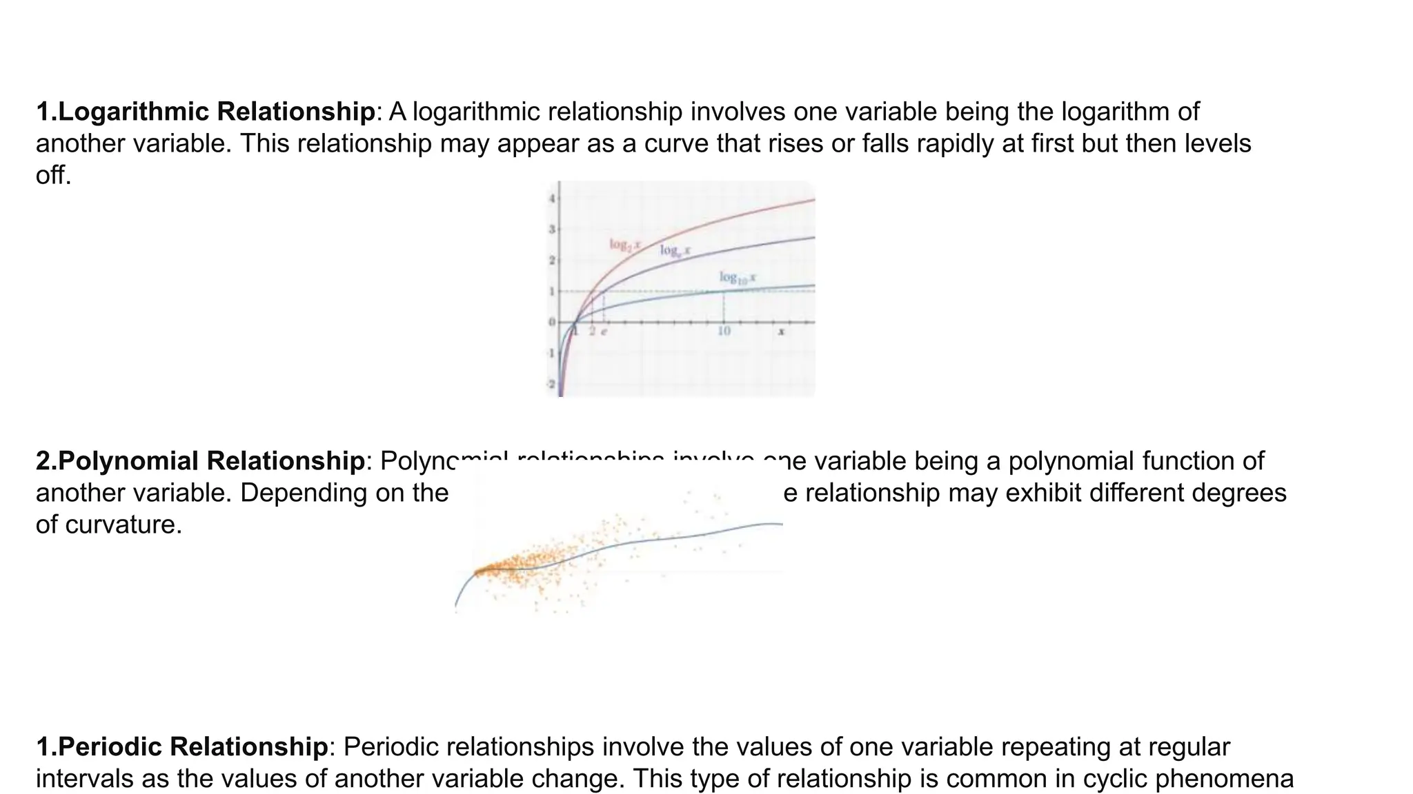
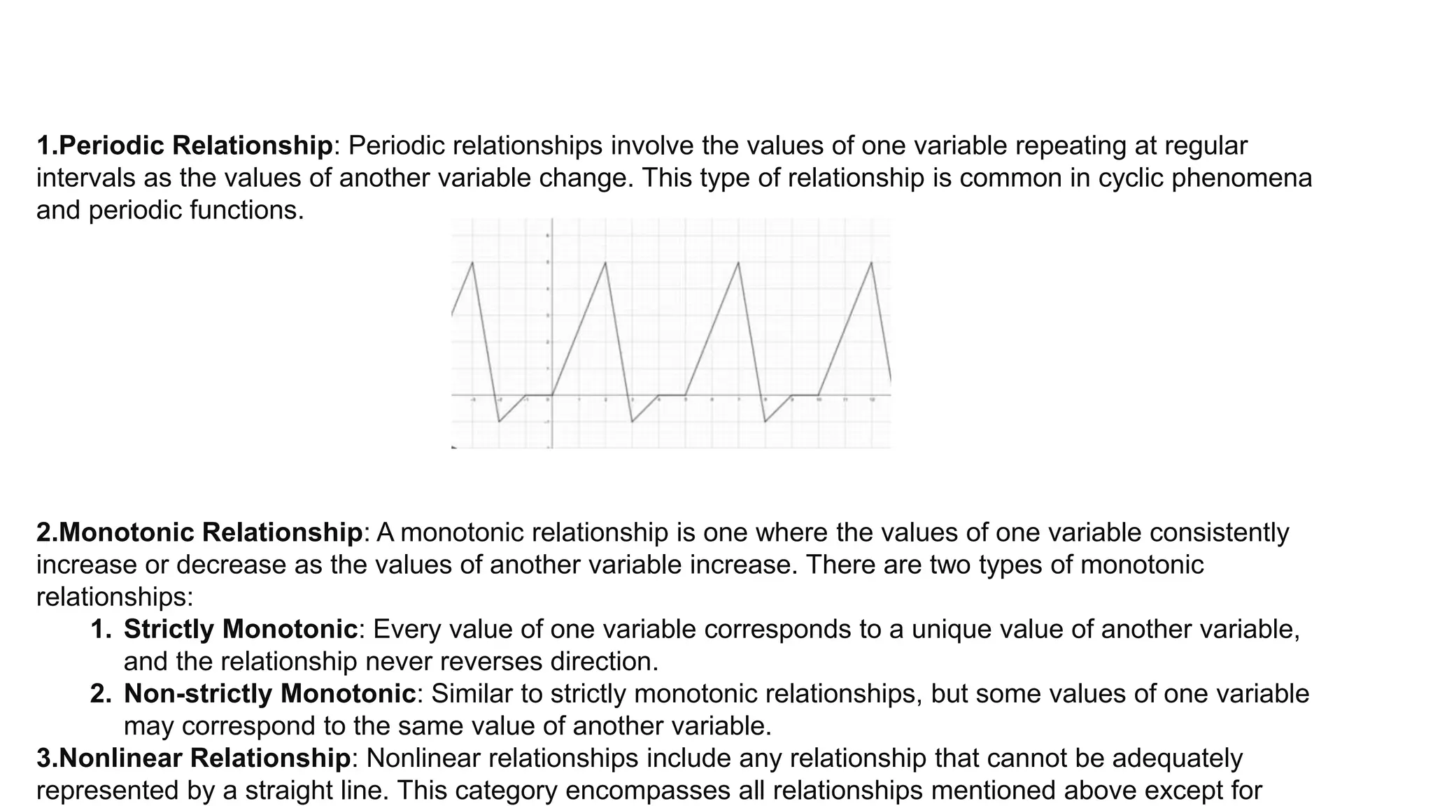
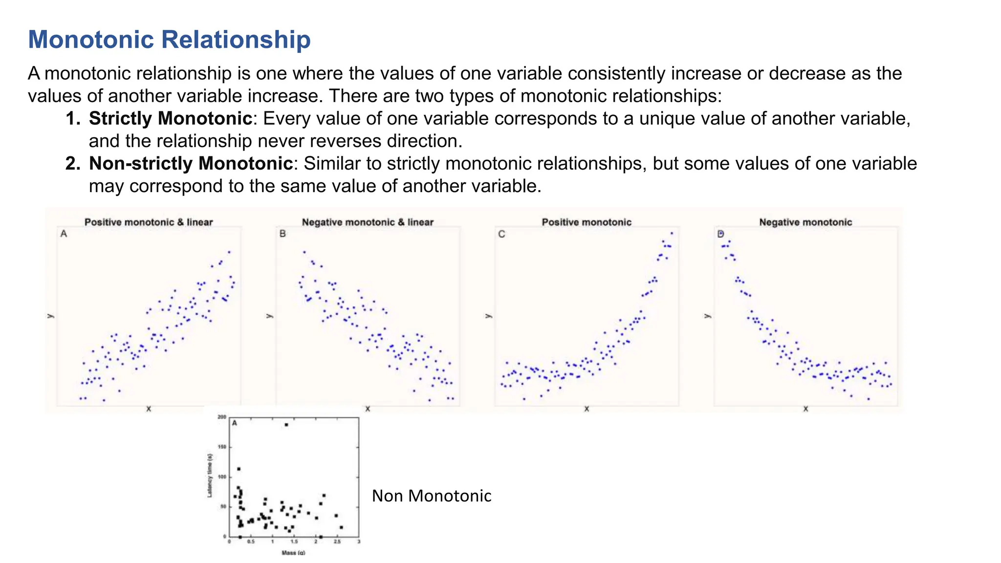
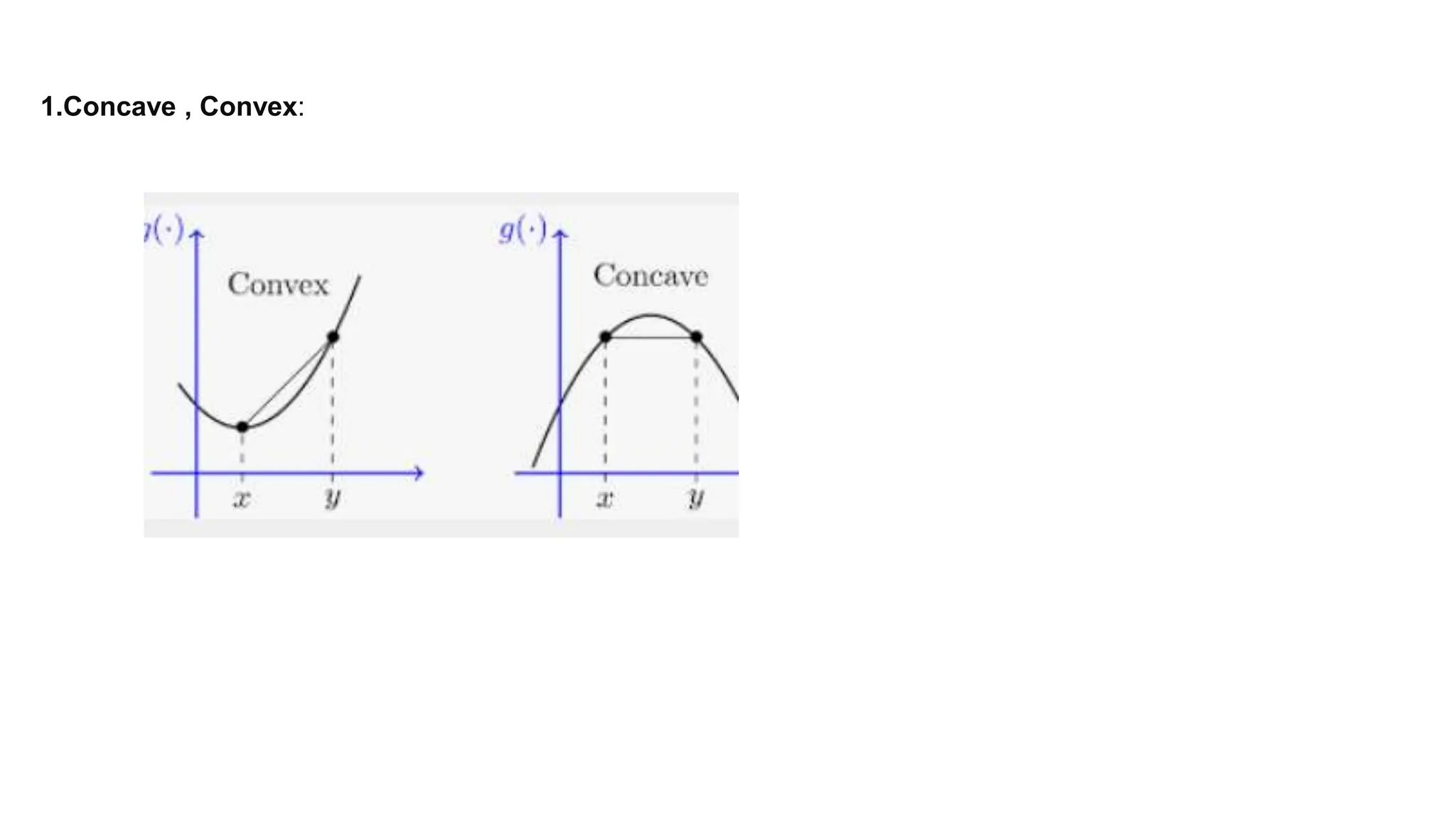
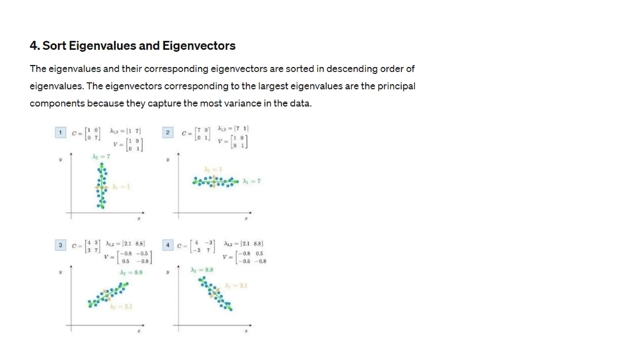
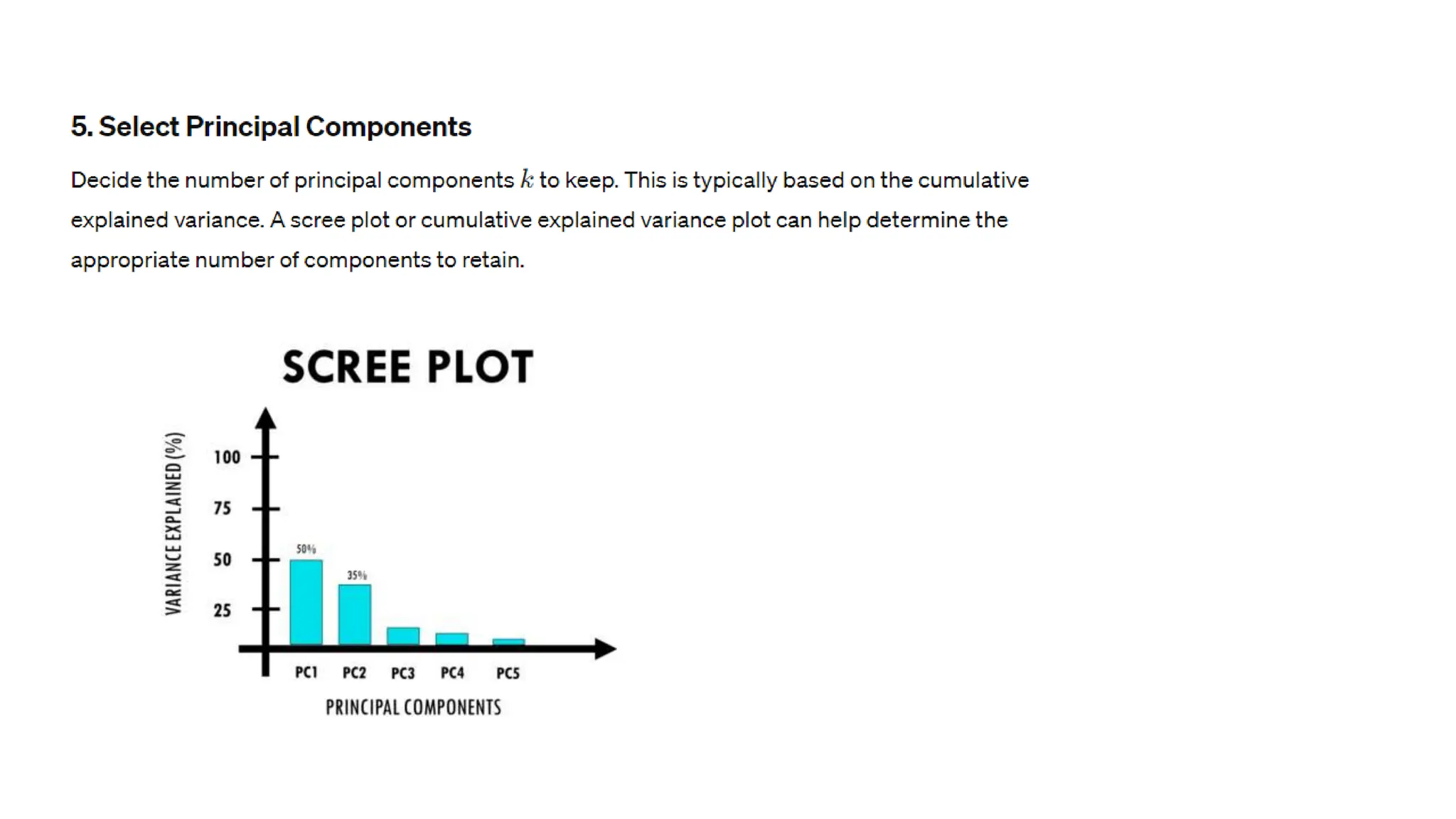
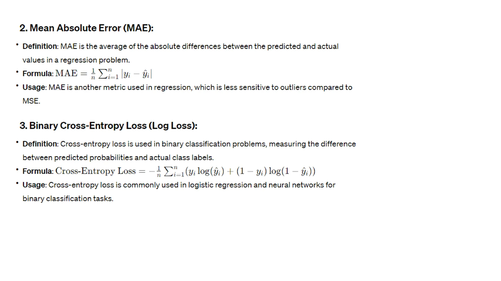
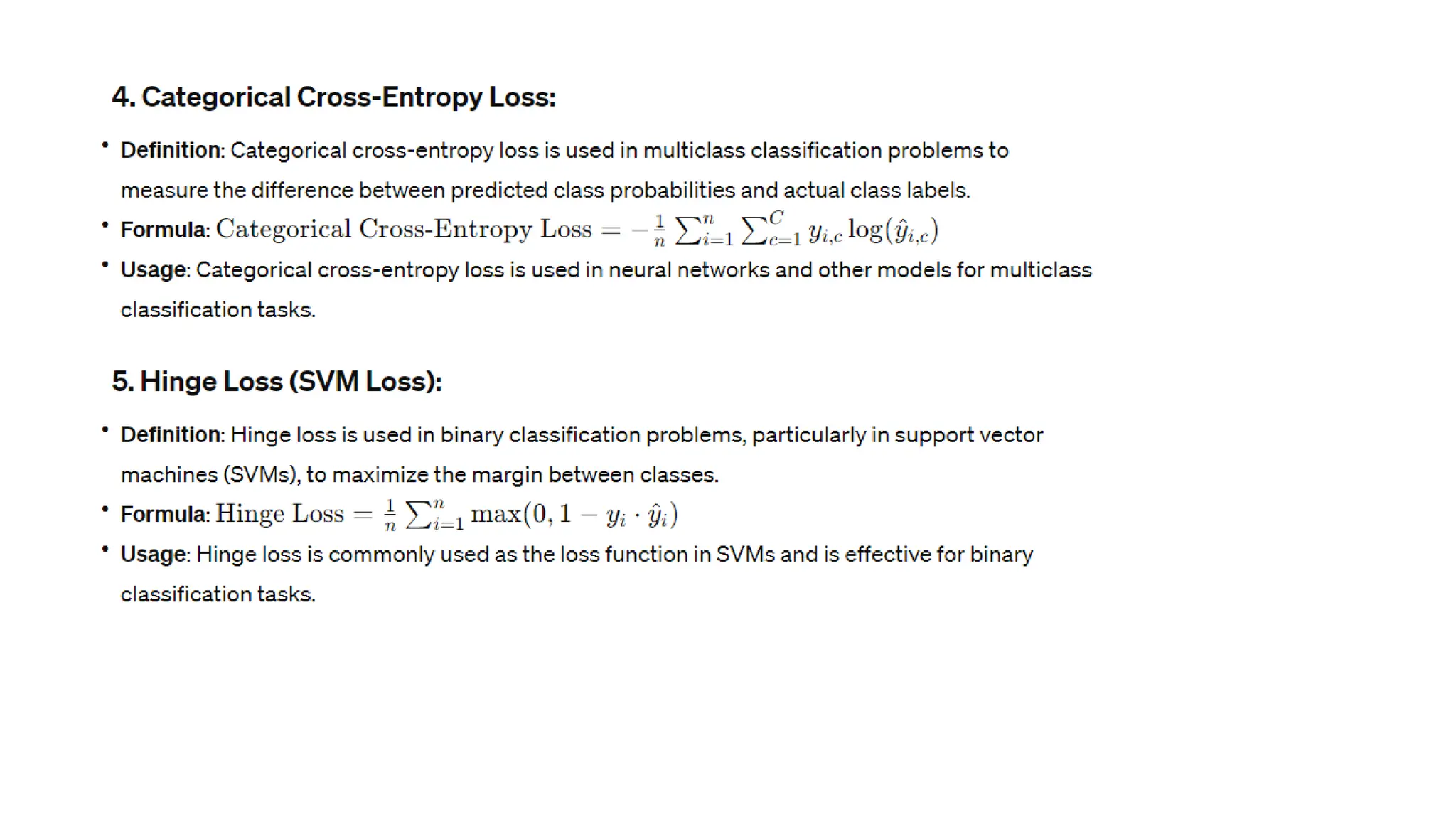
Download to read offline

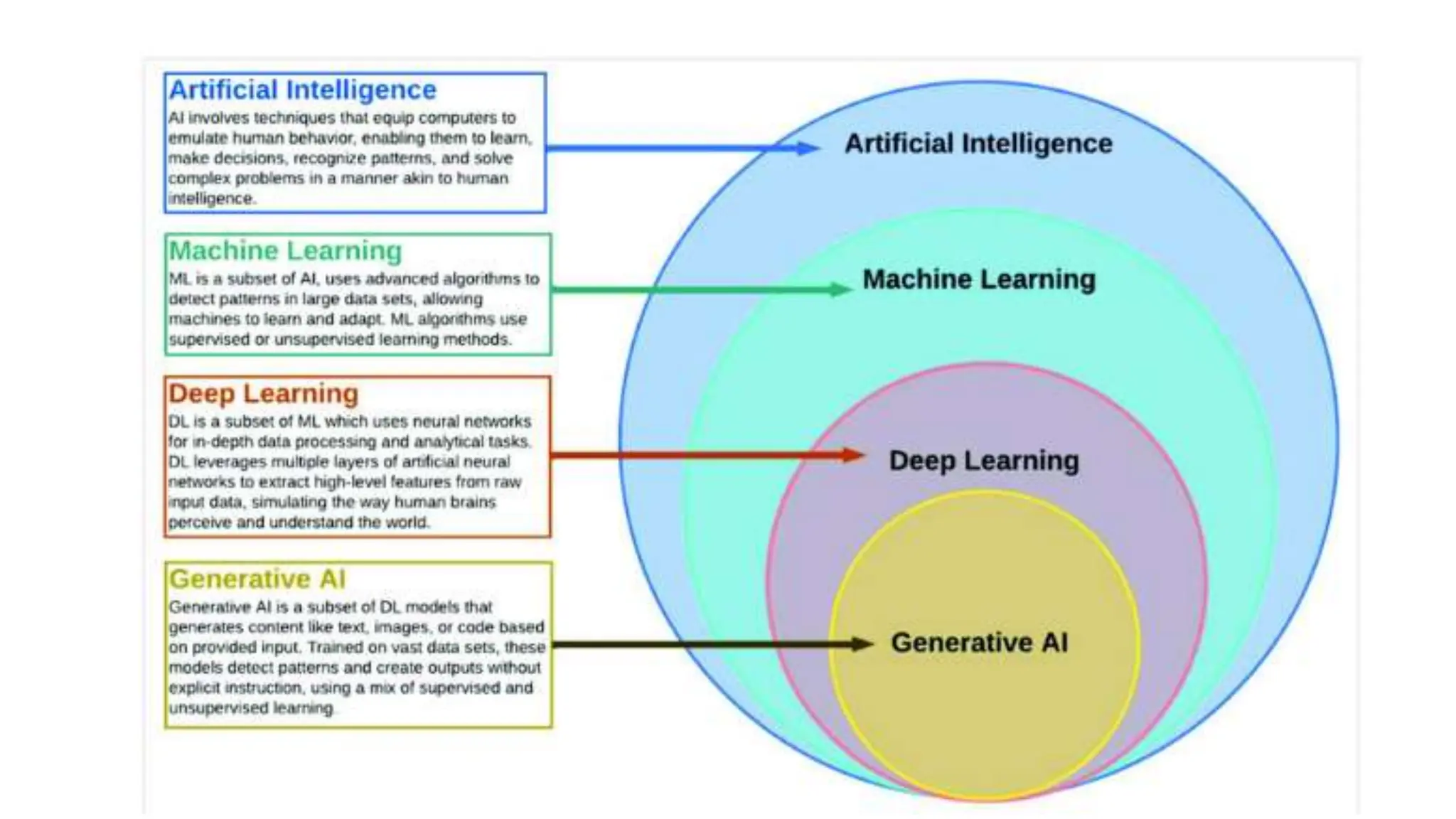

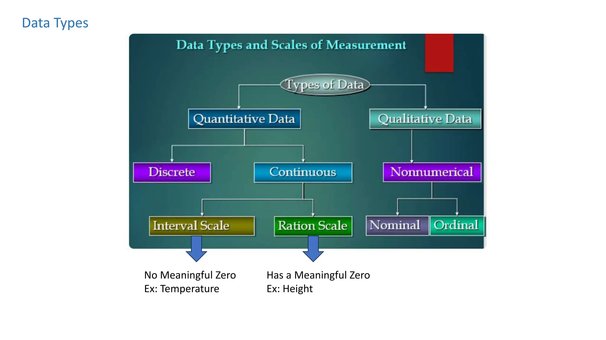
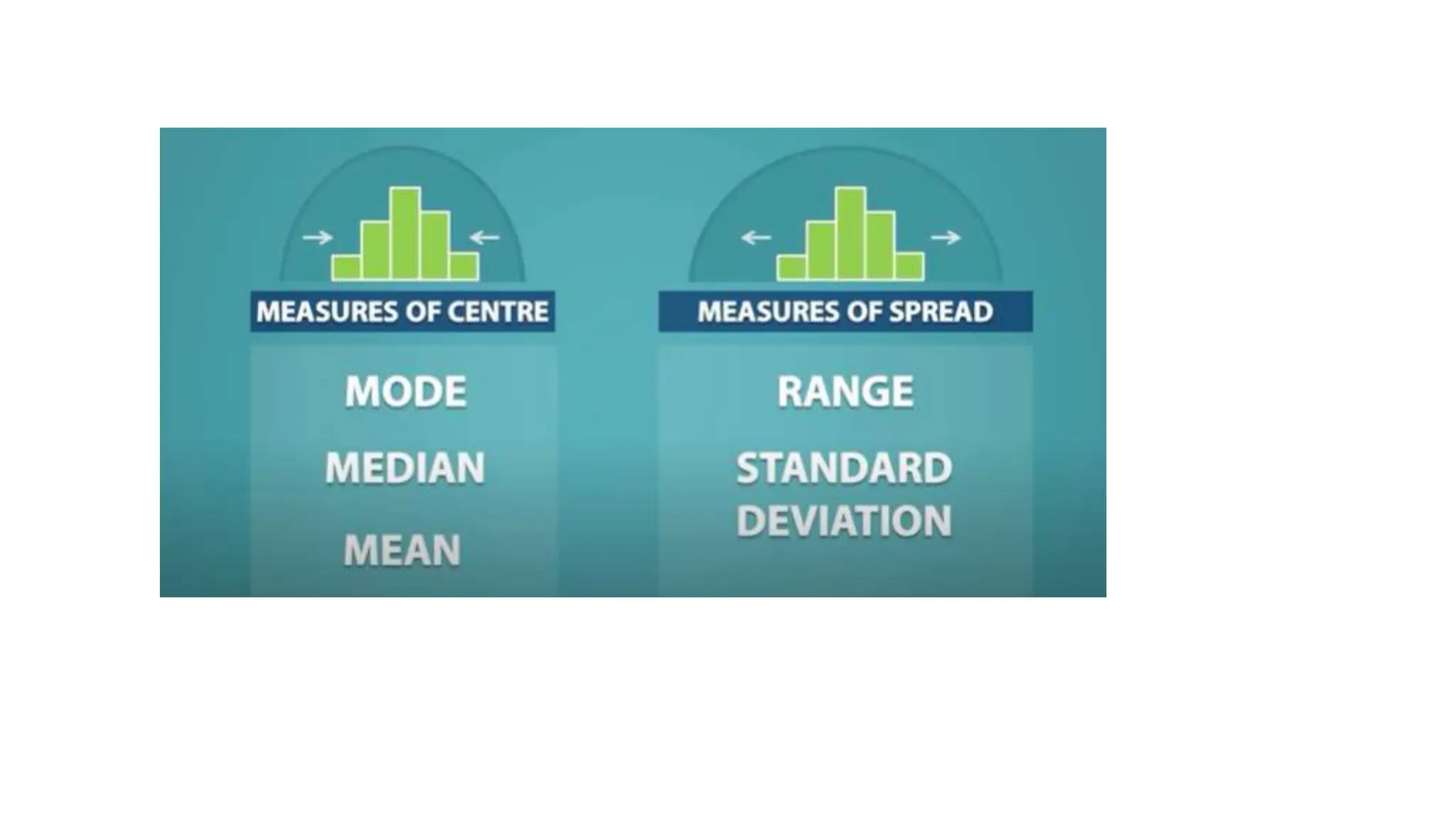
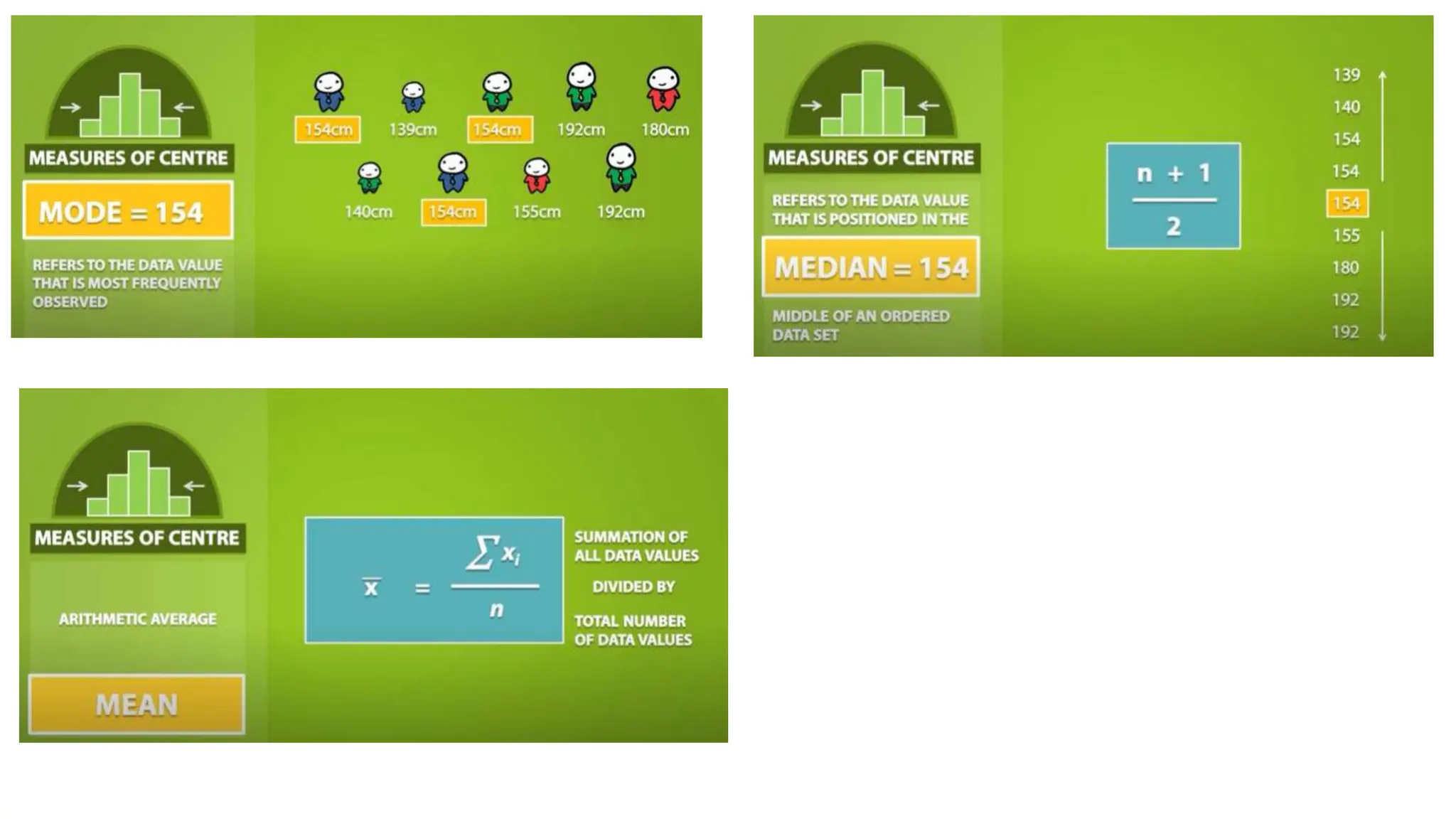
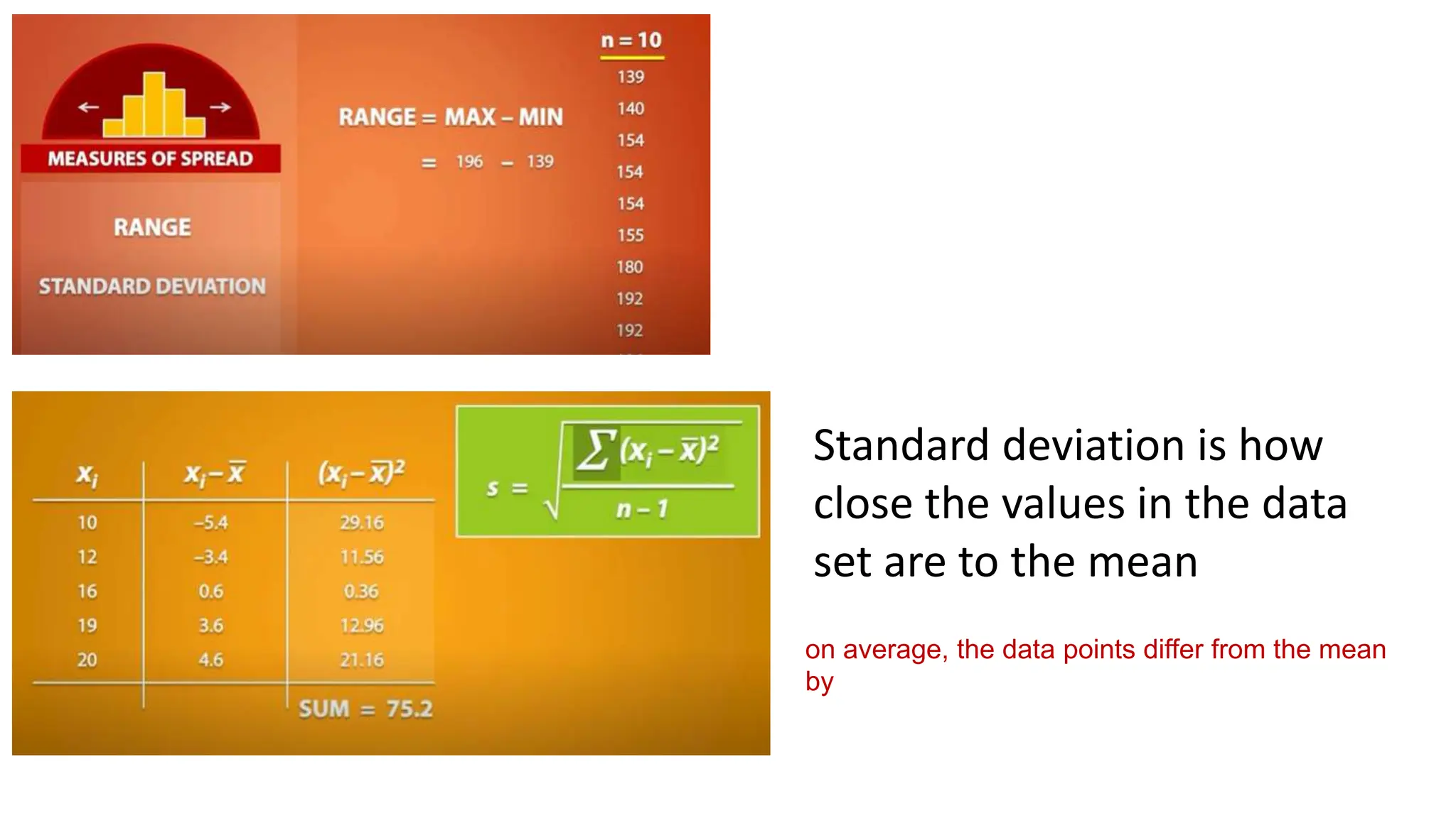
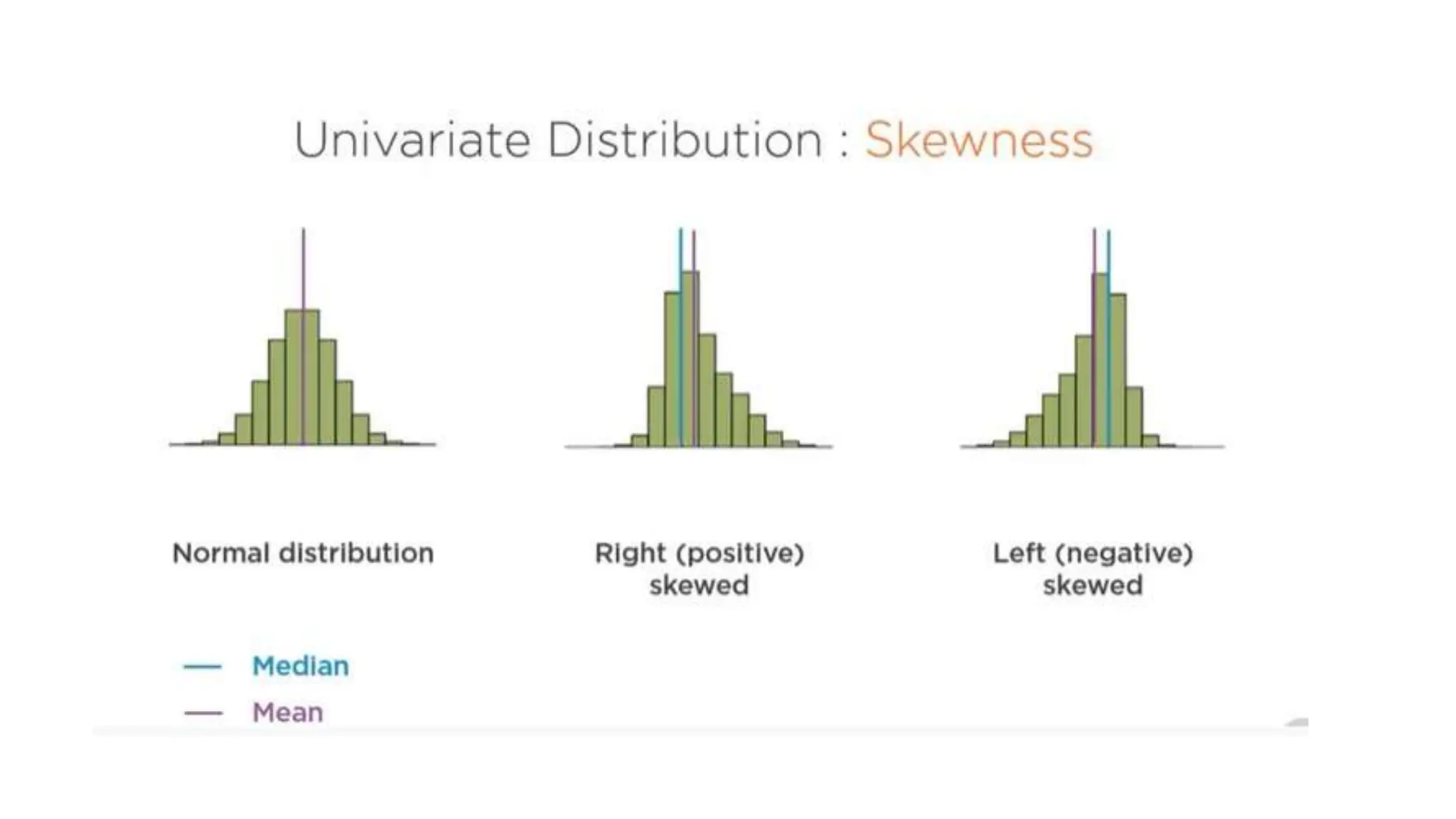
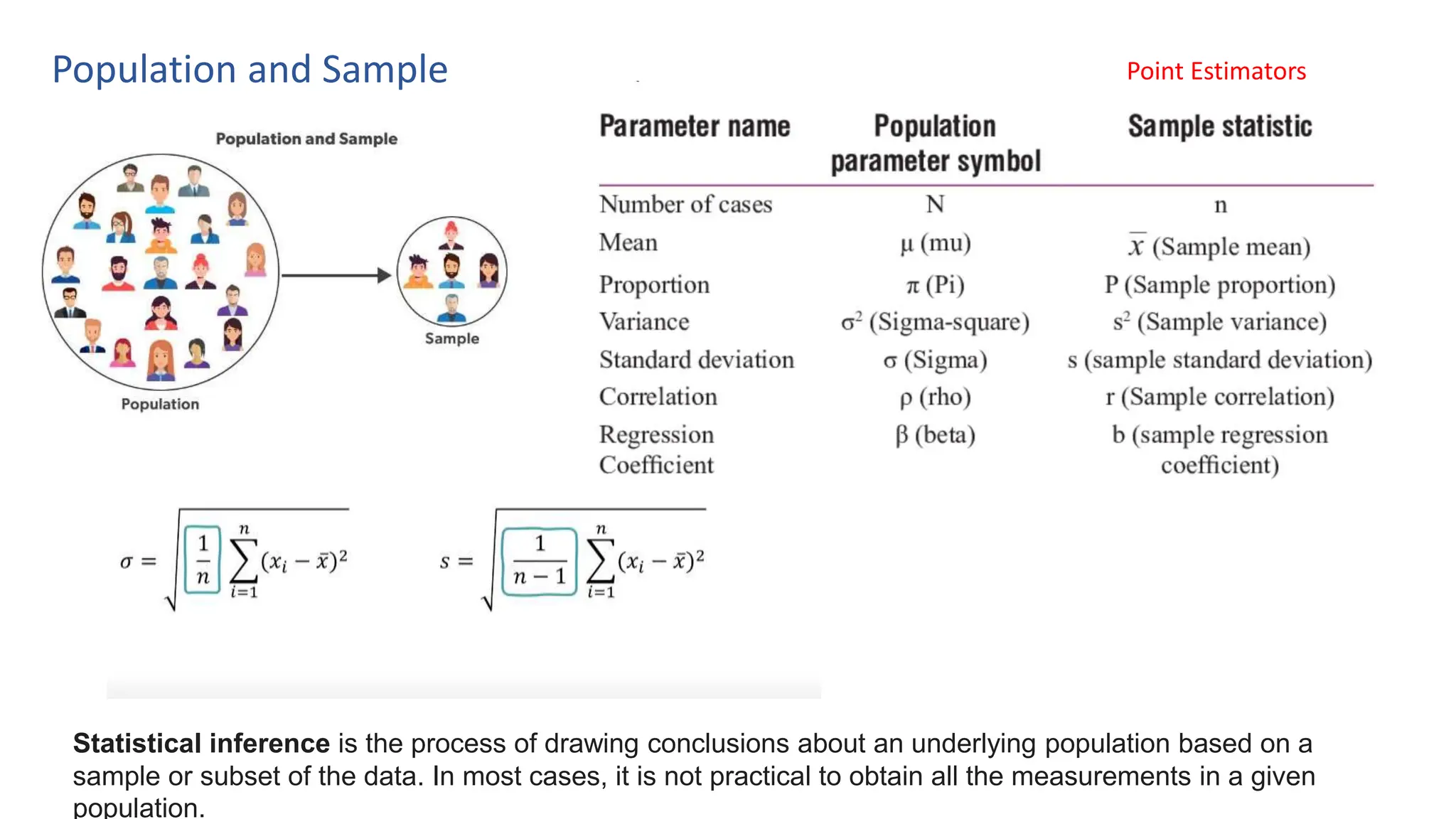
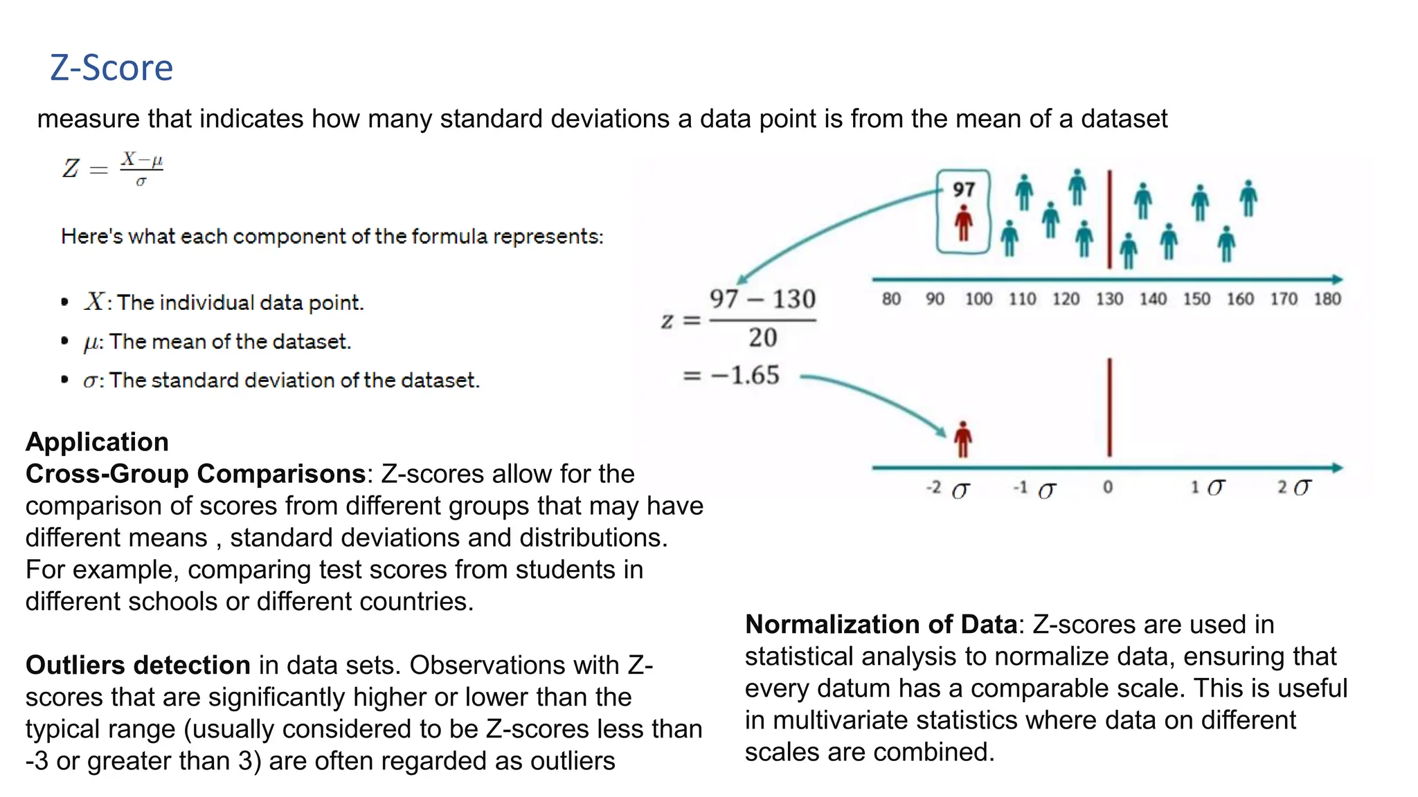
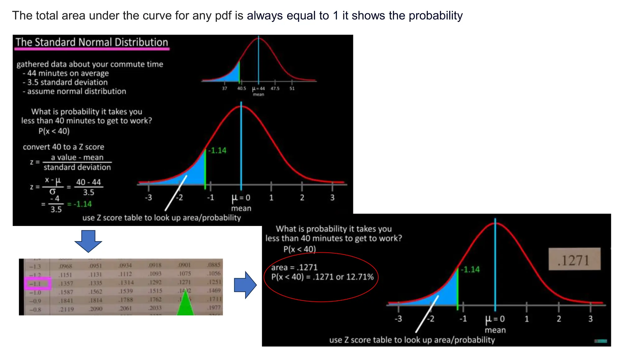
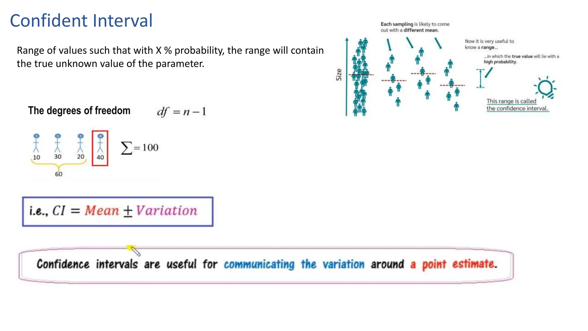
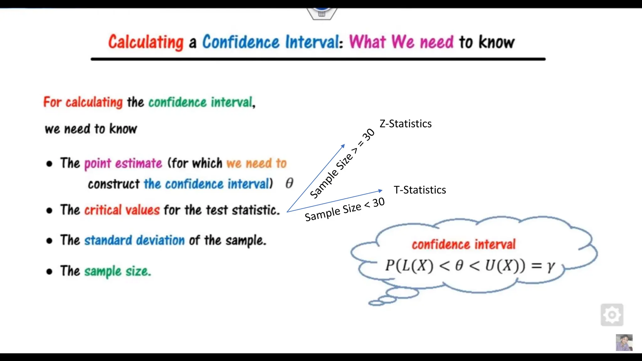
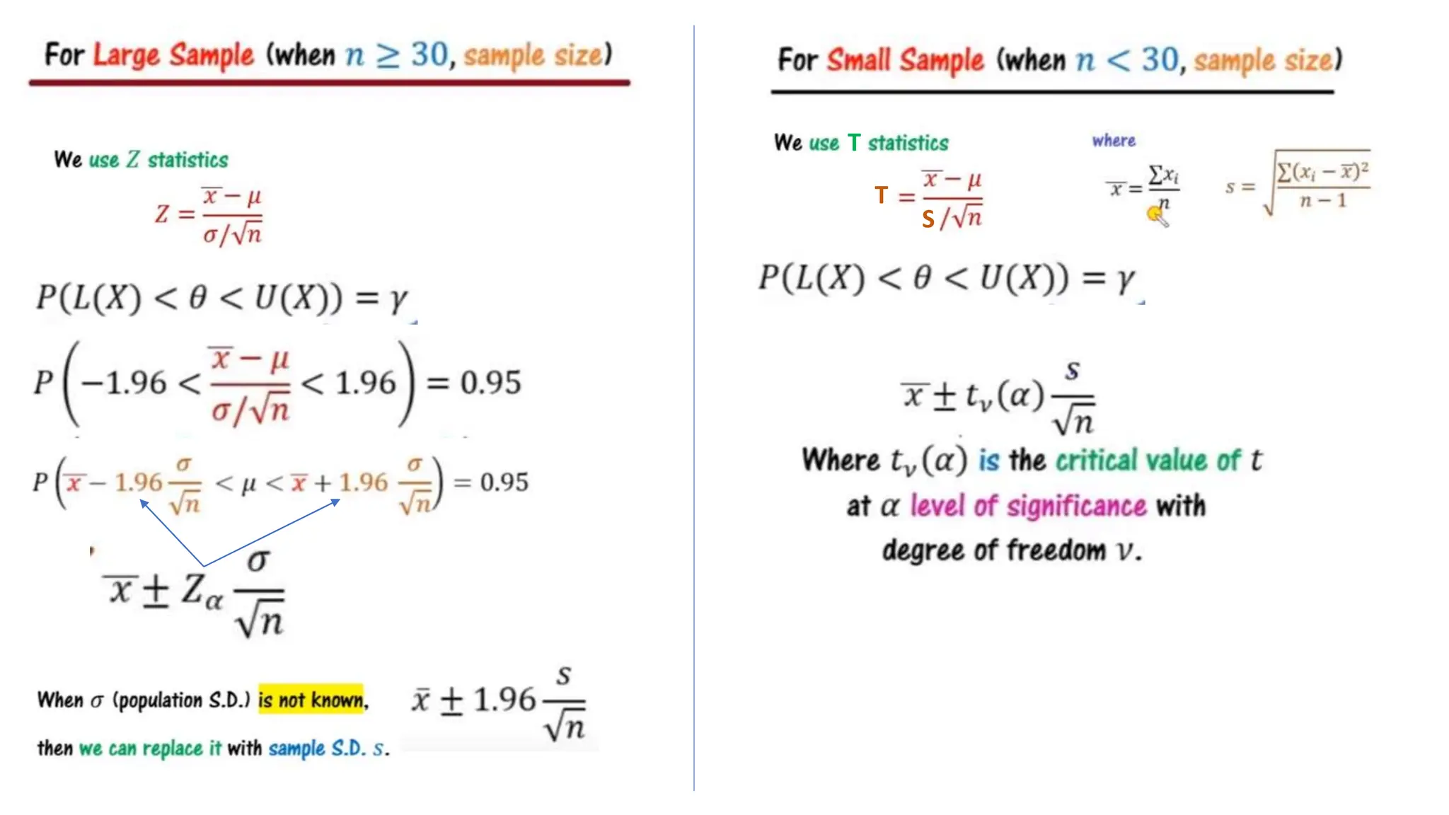
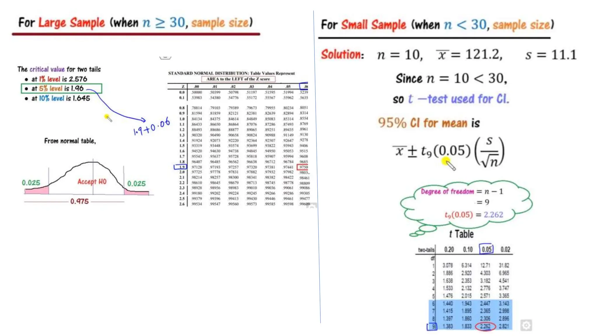
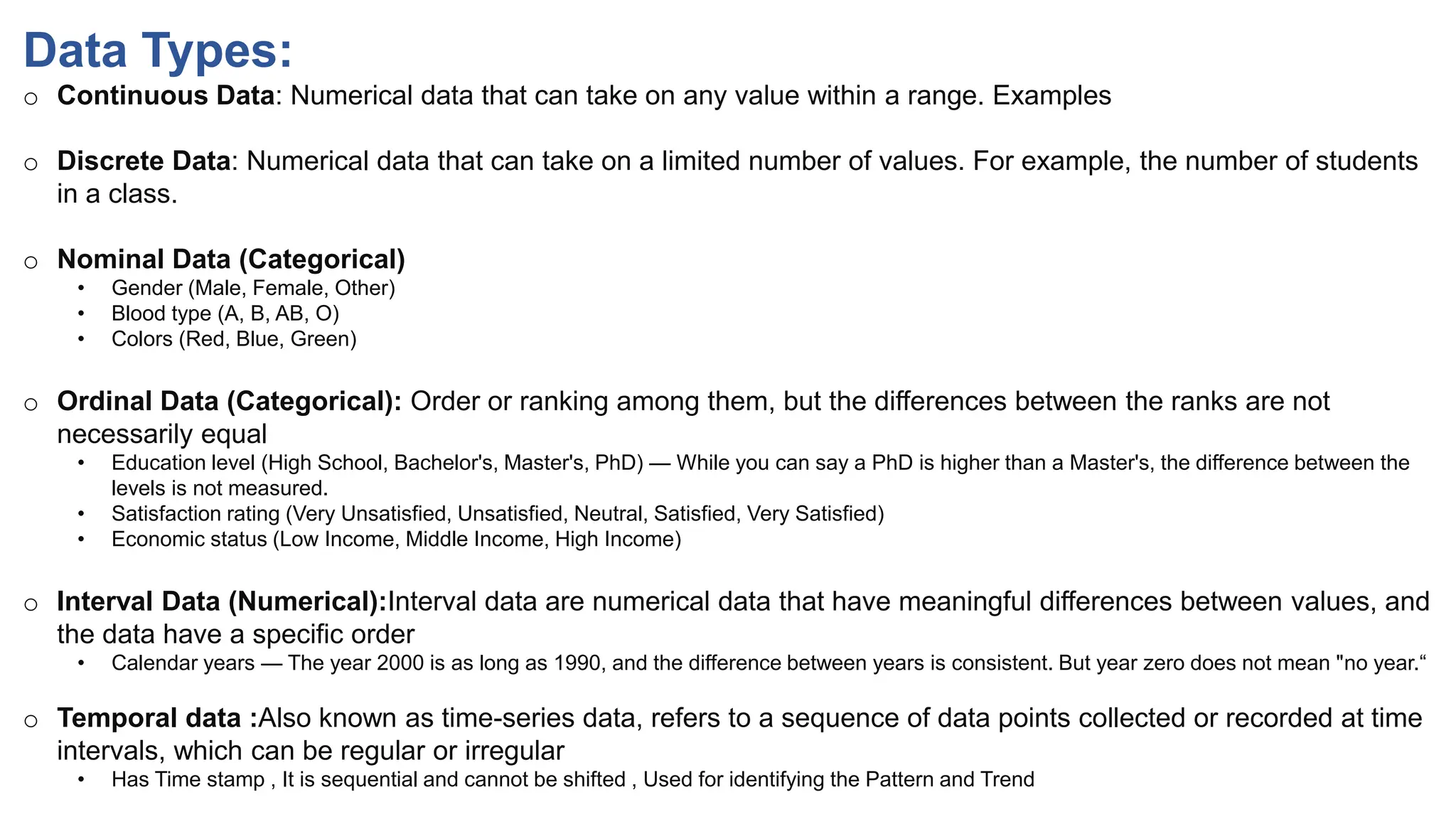
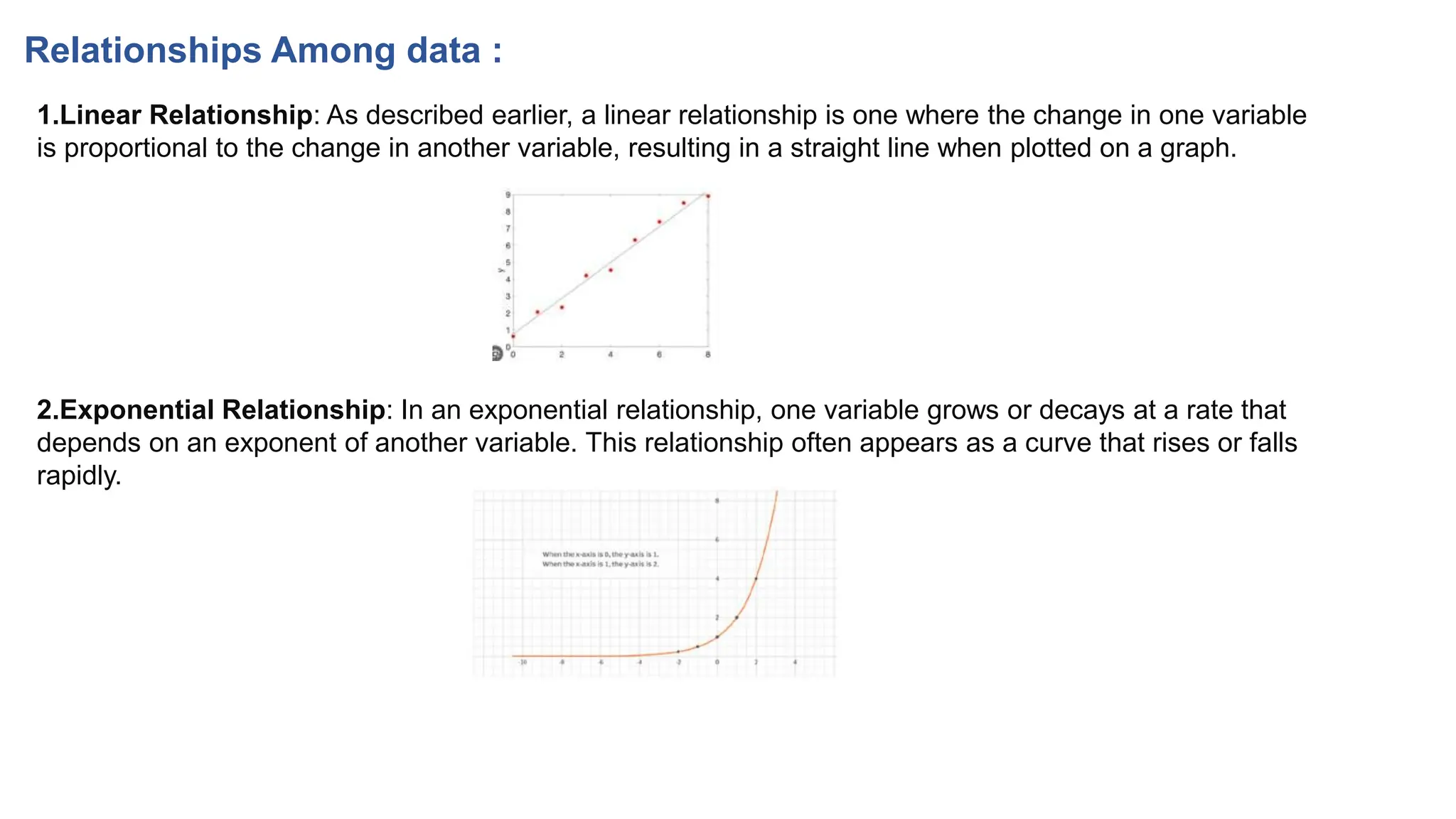

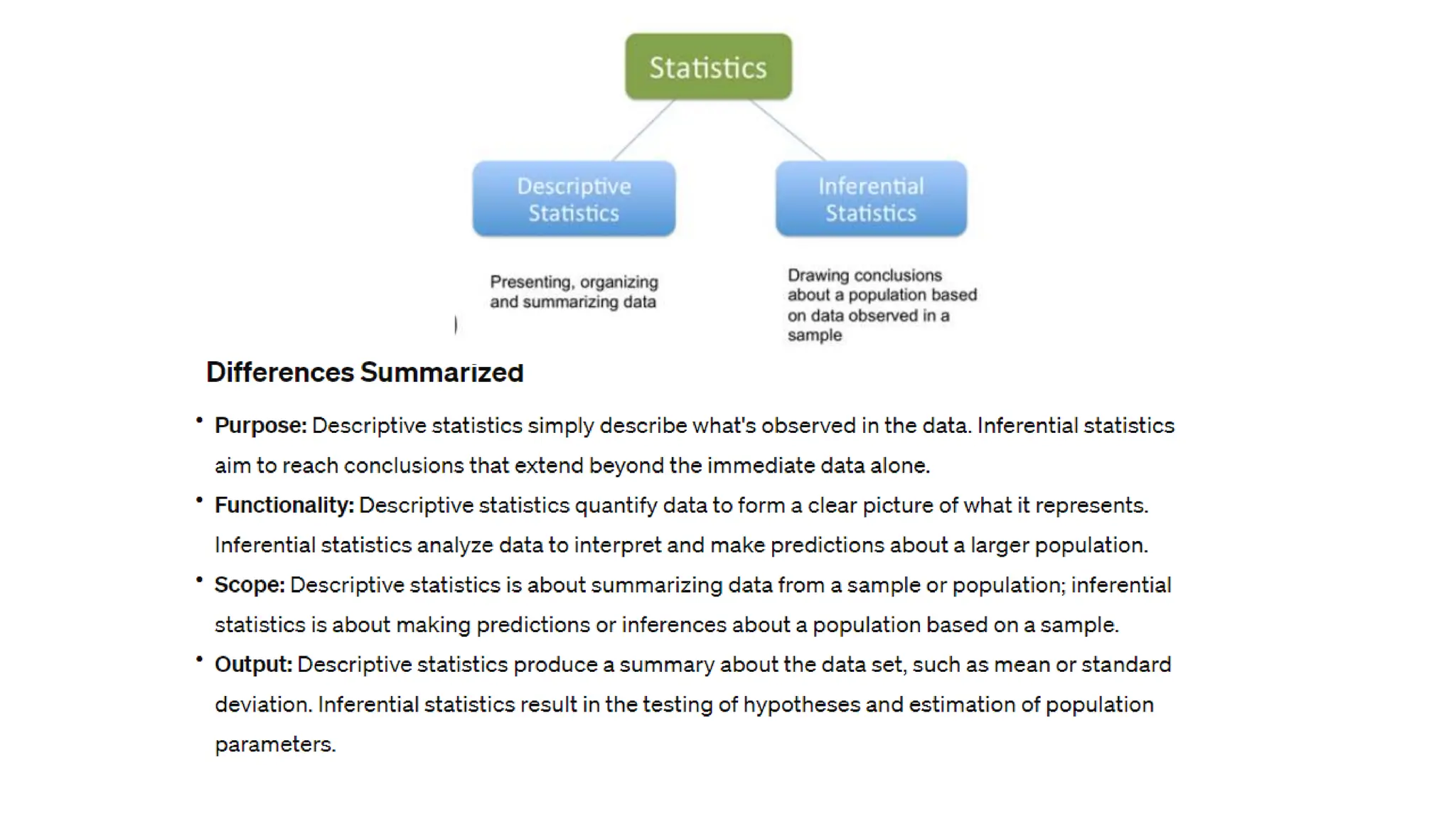
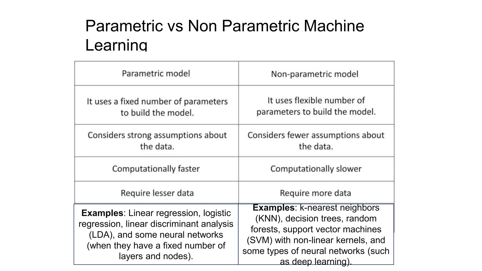
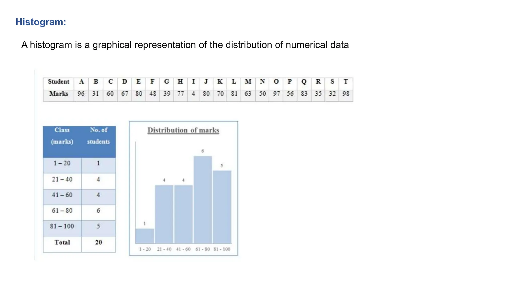
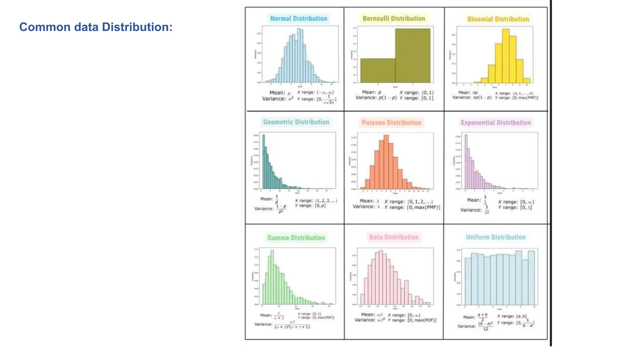
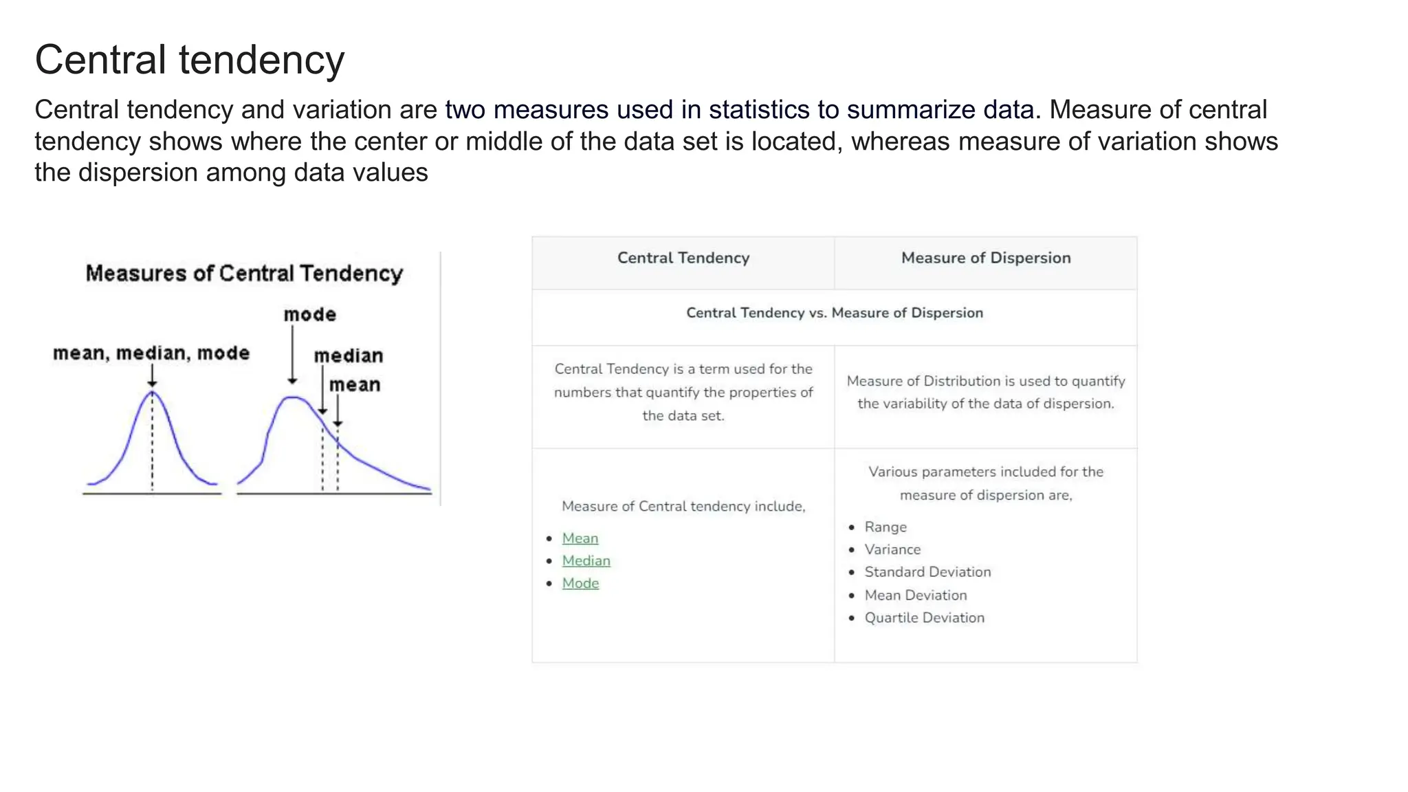
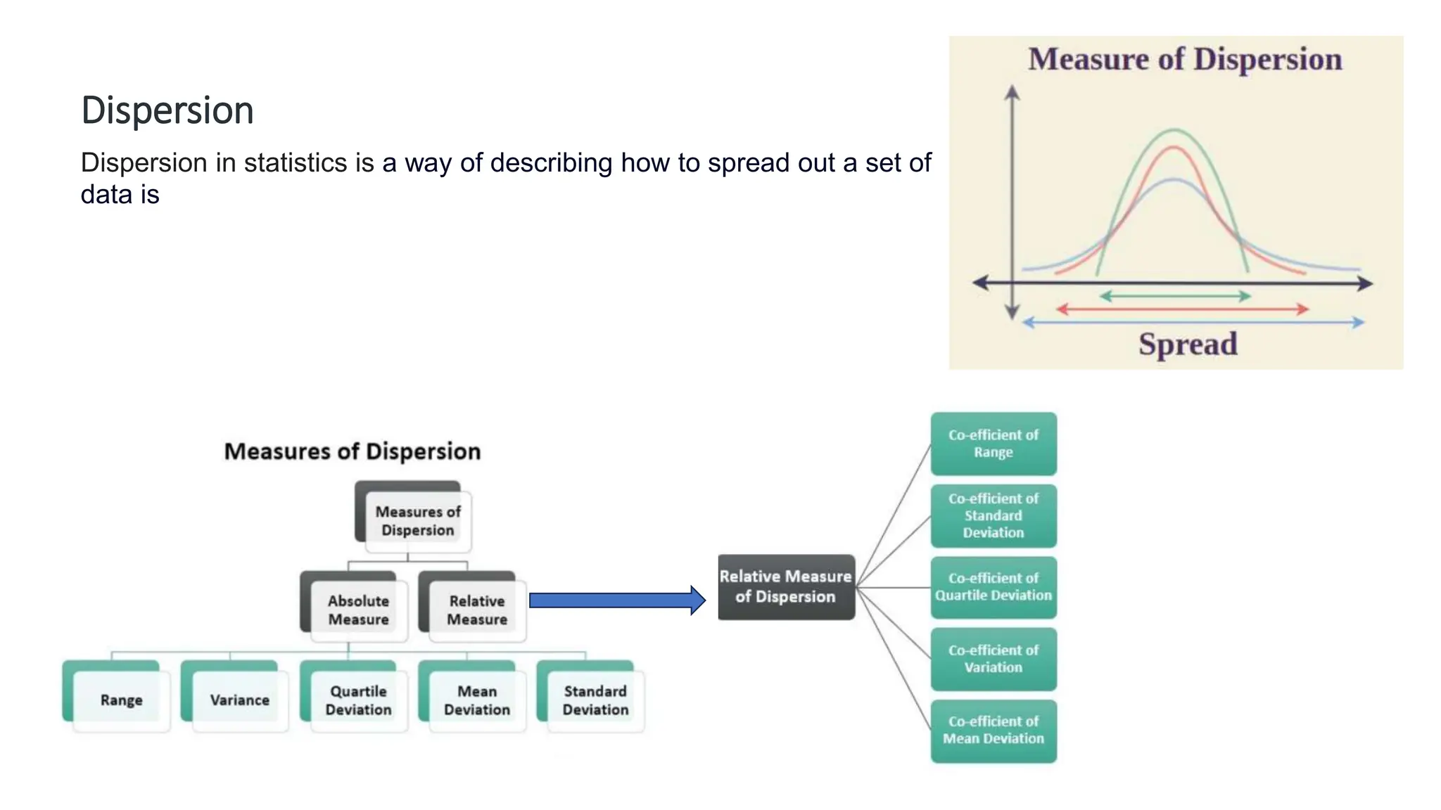
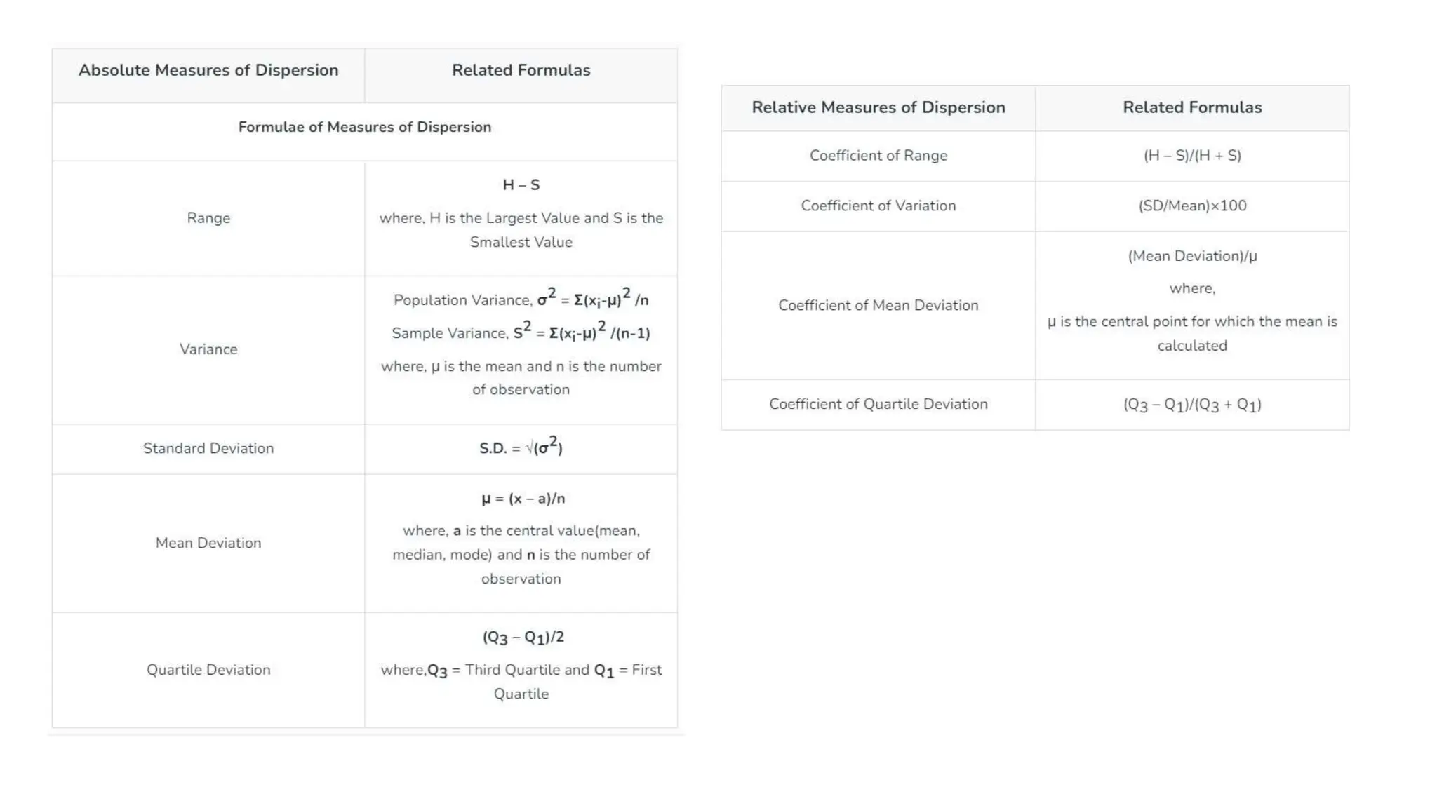
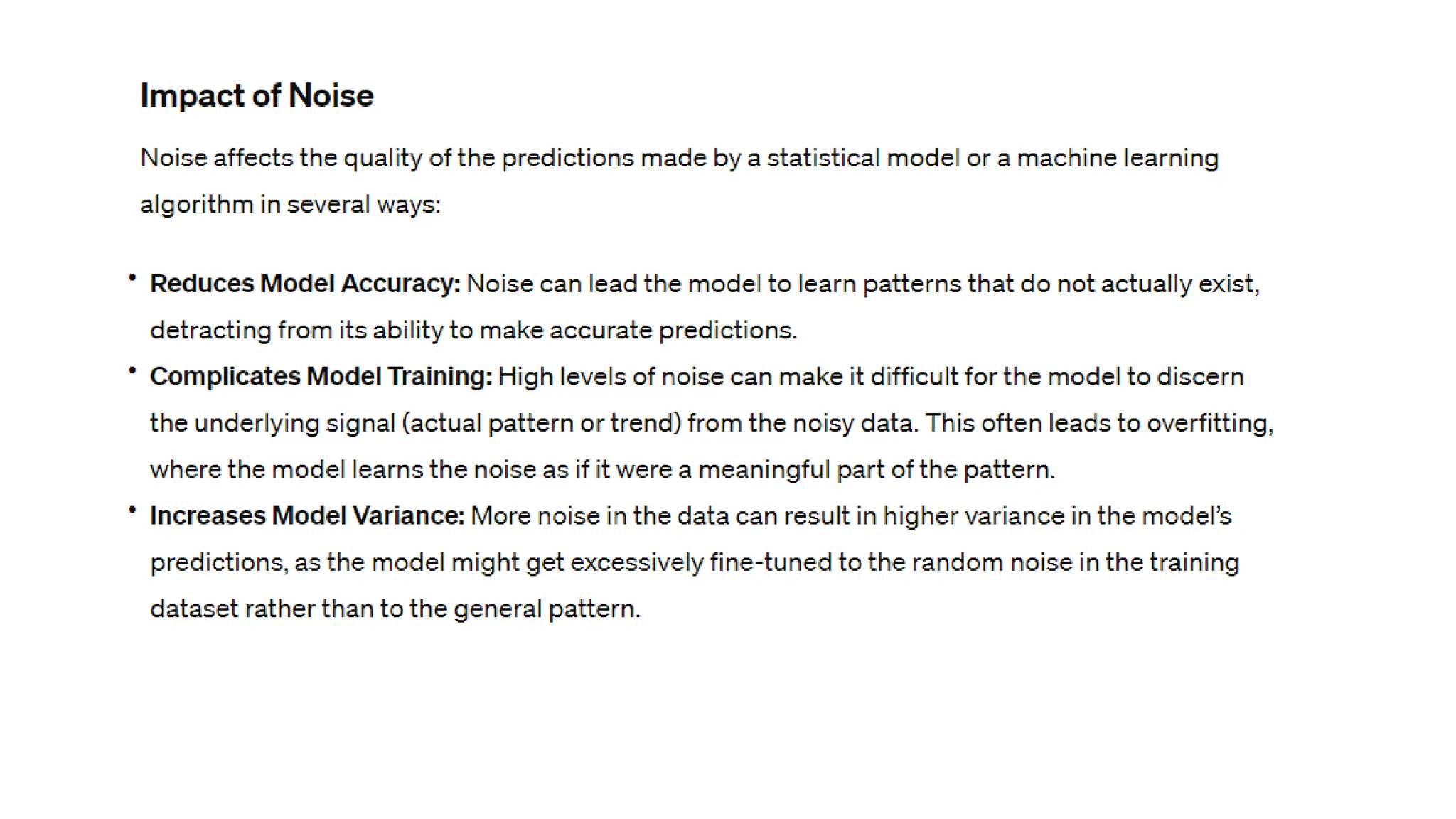
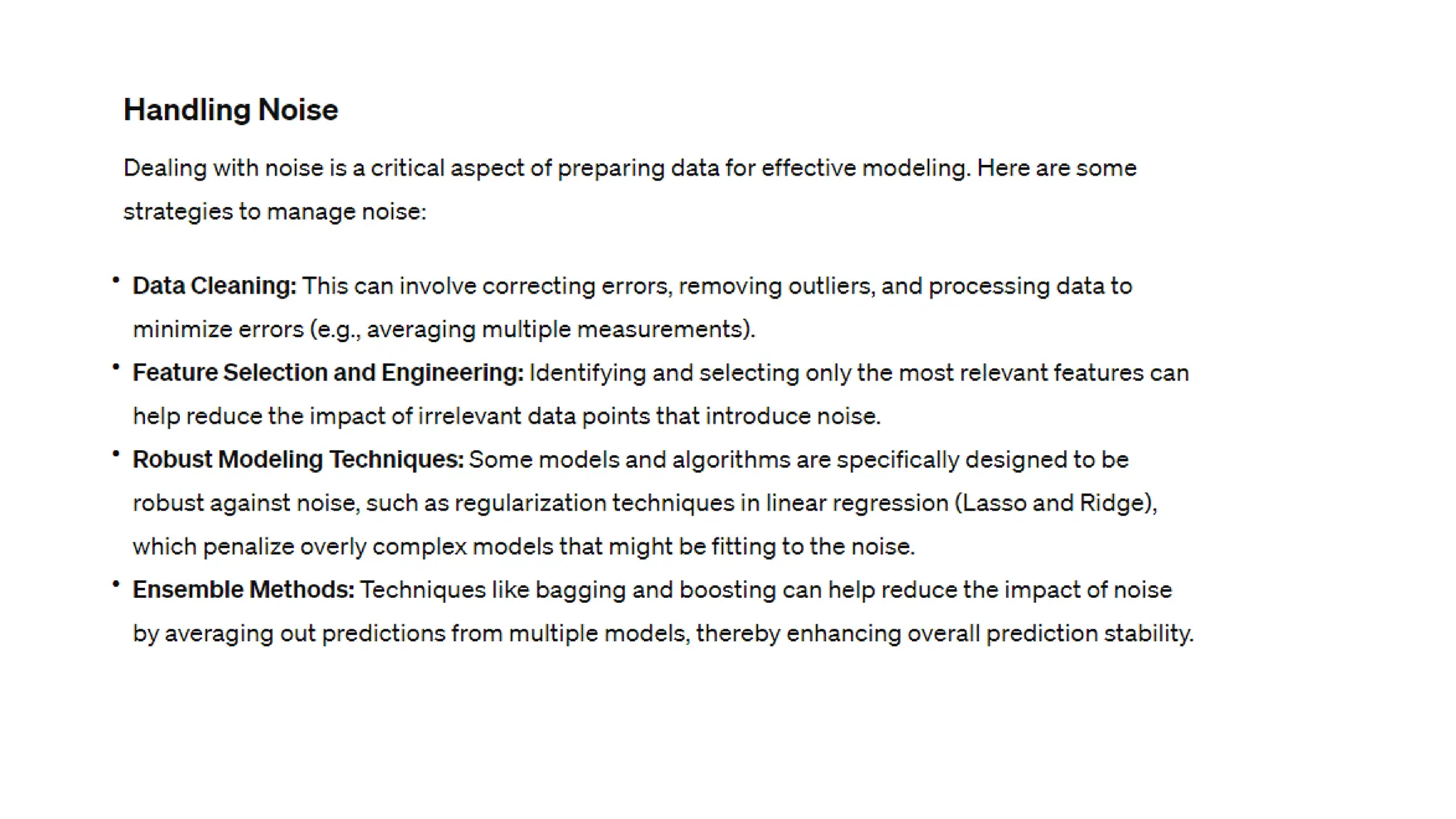

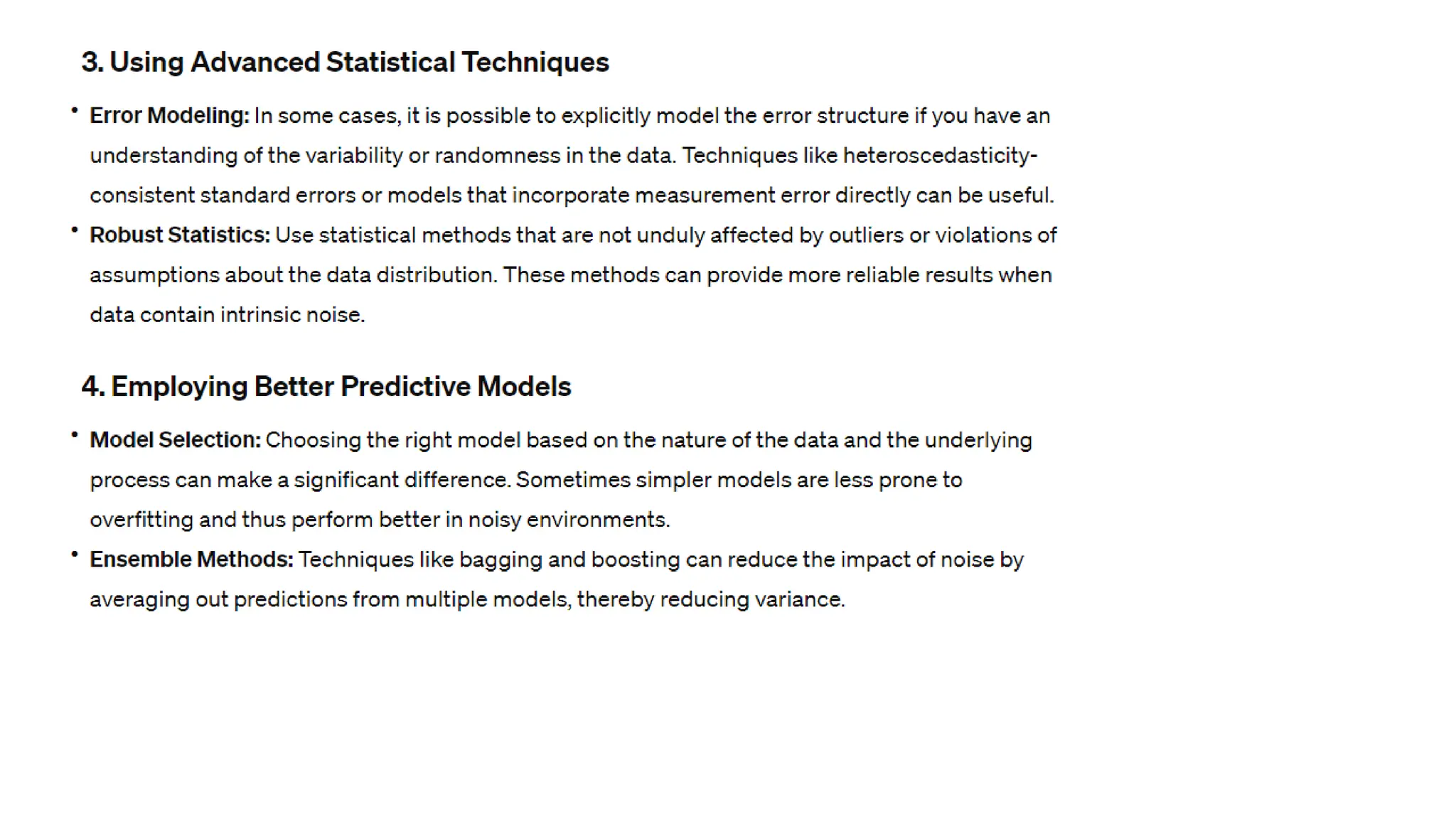
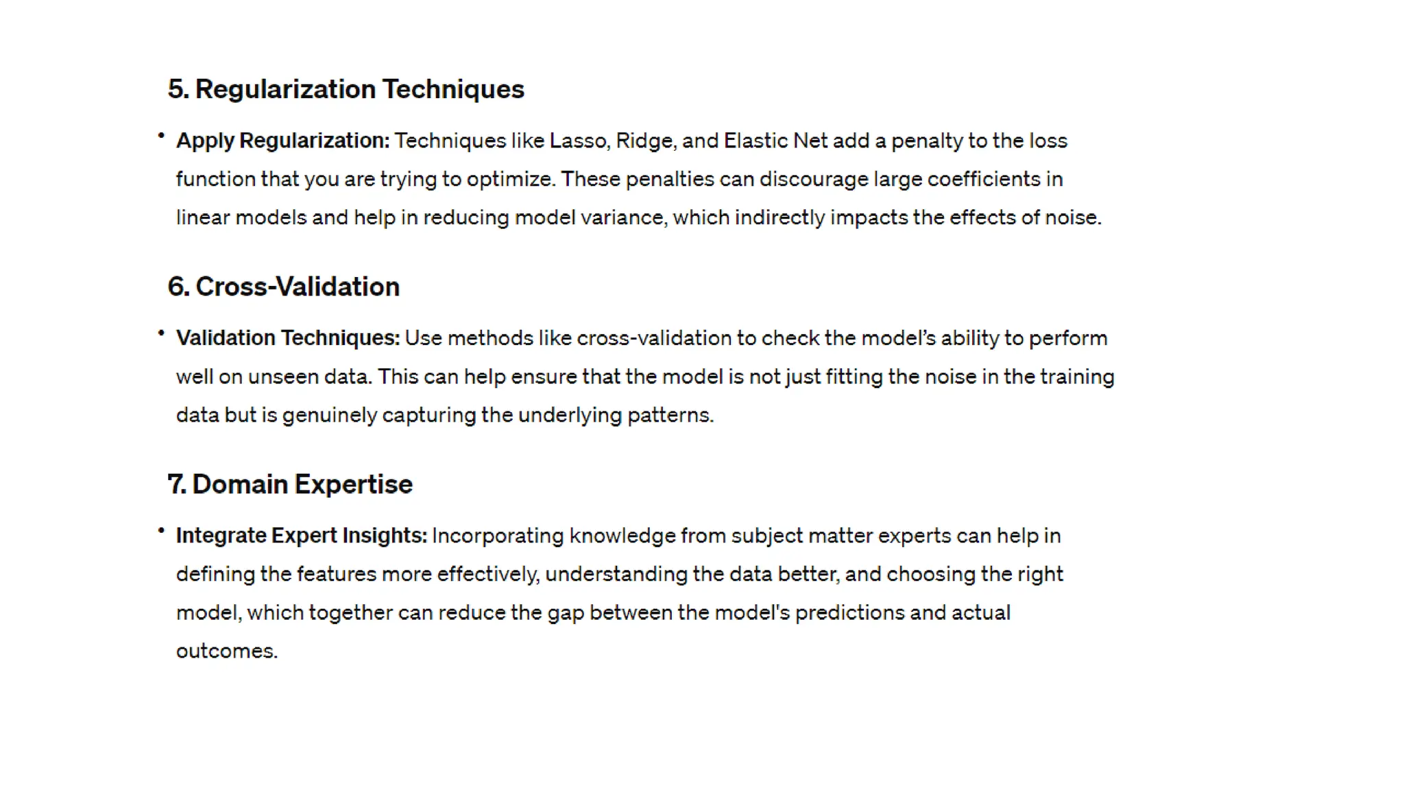

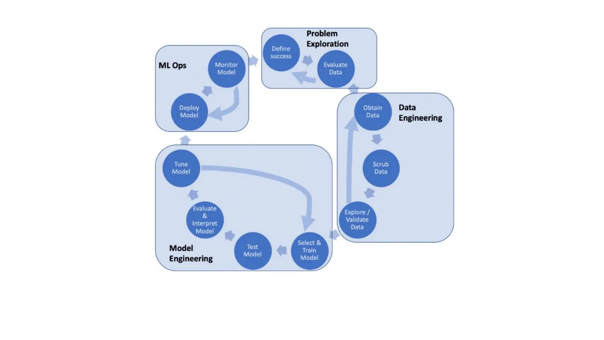

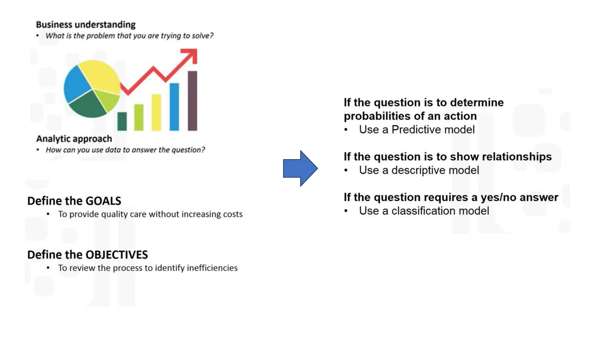
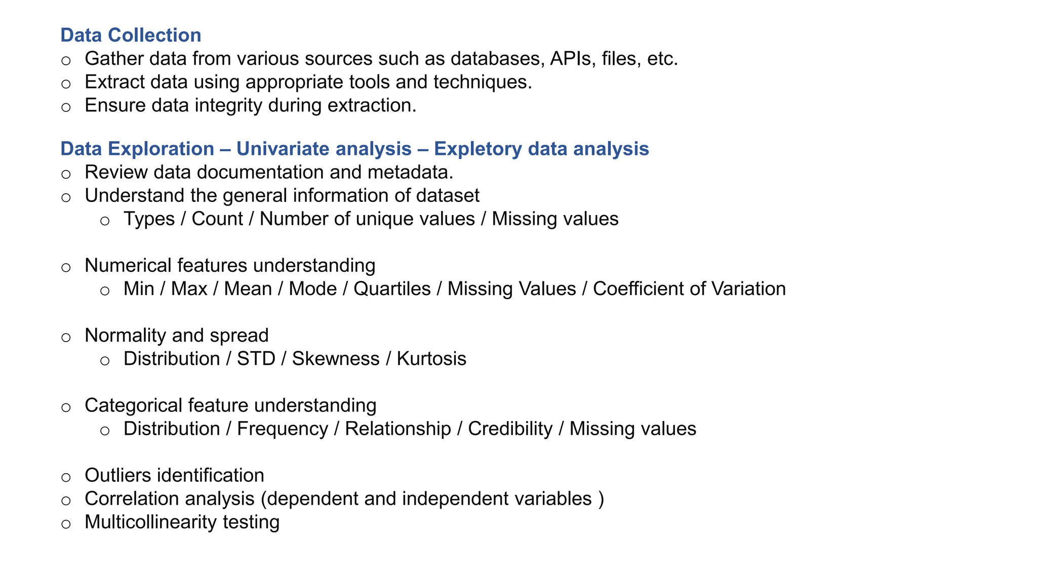
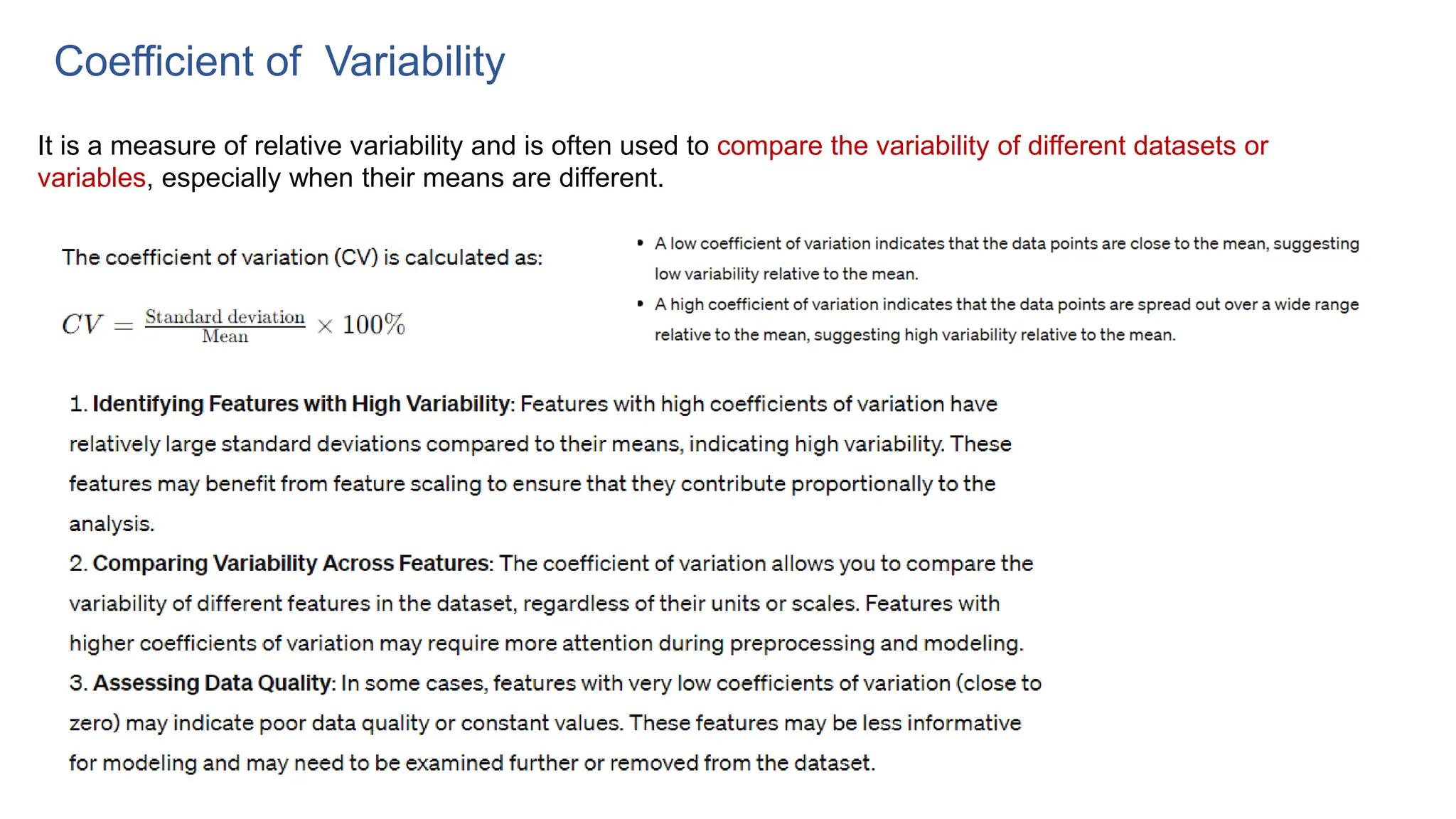

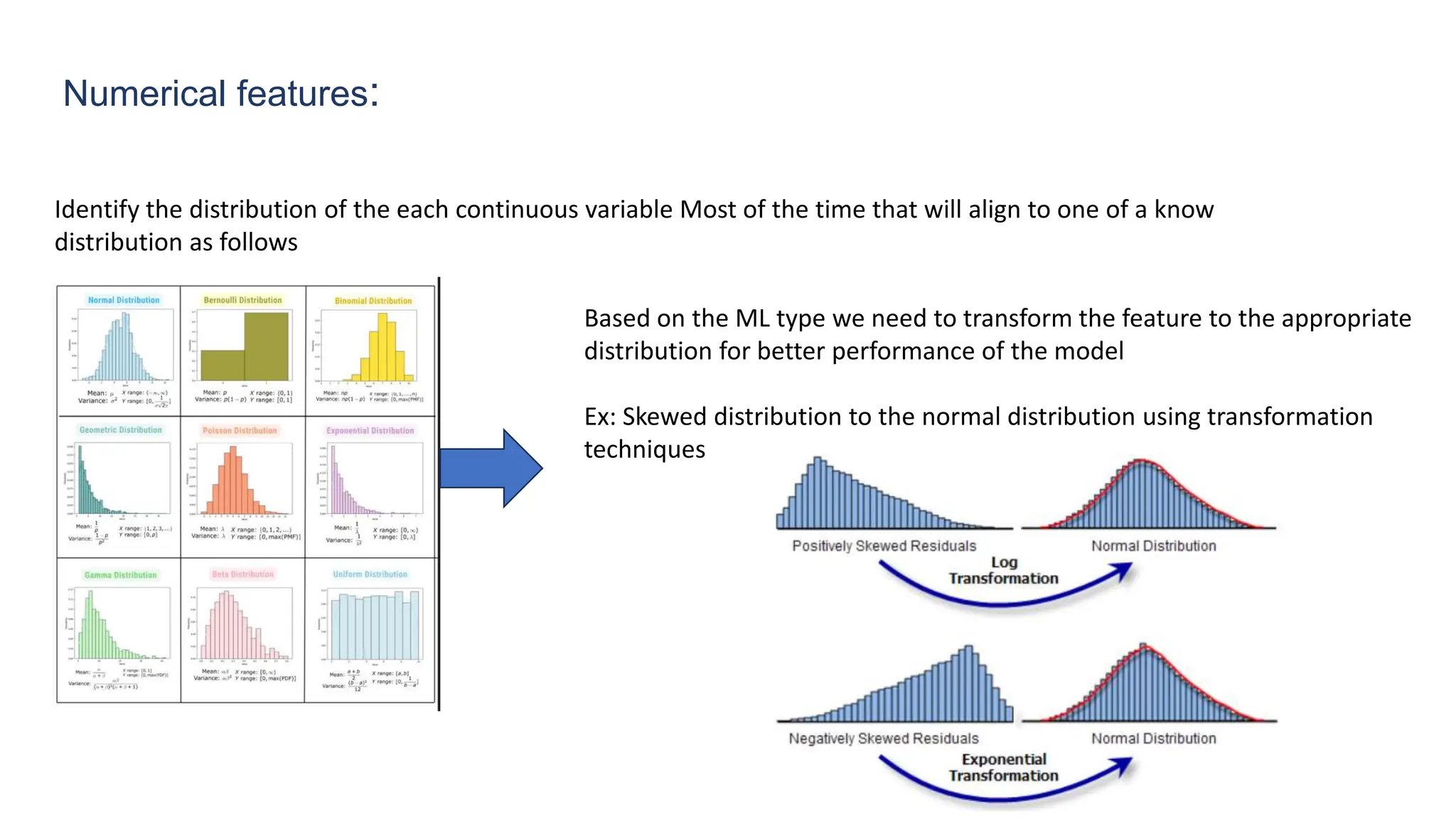

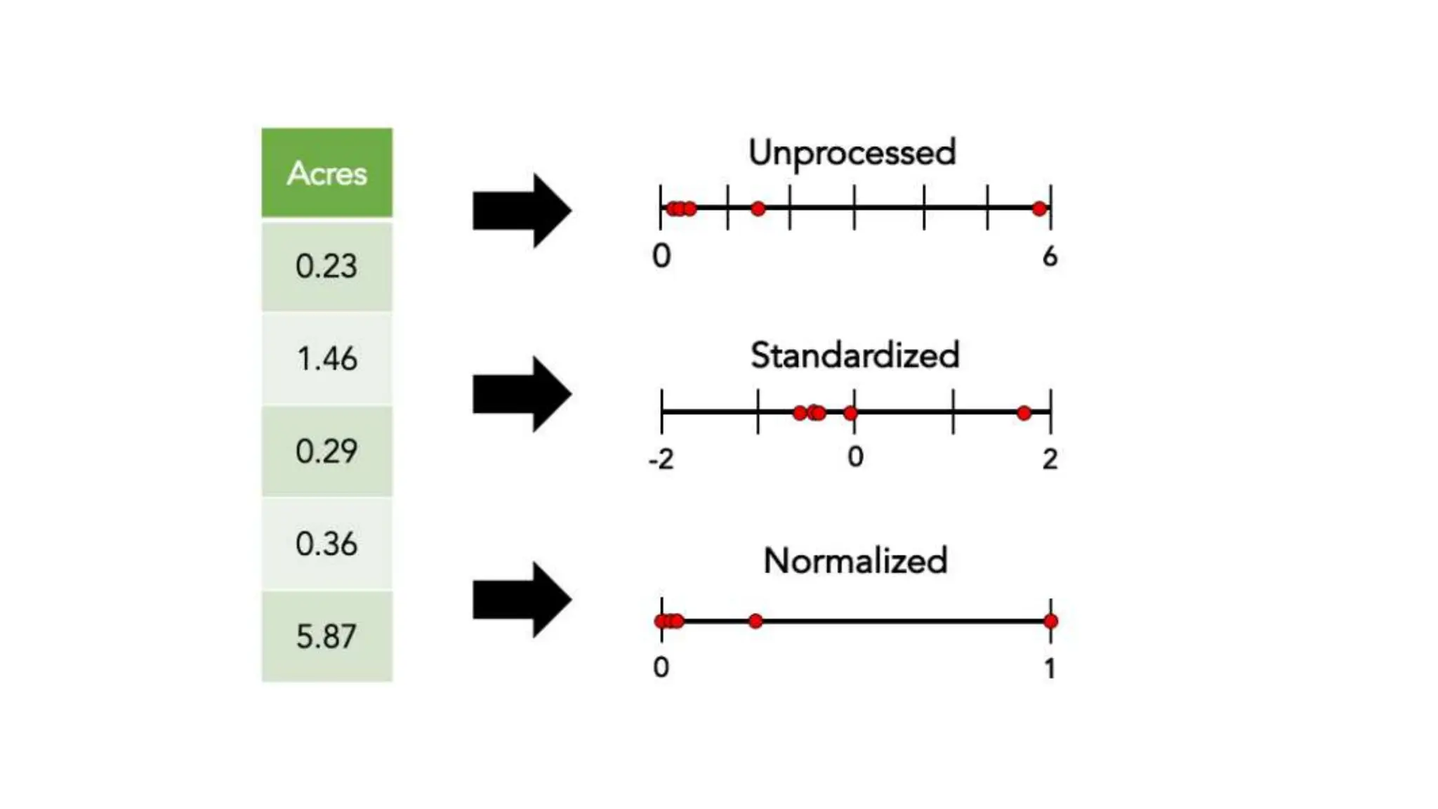
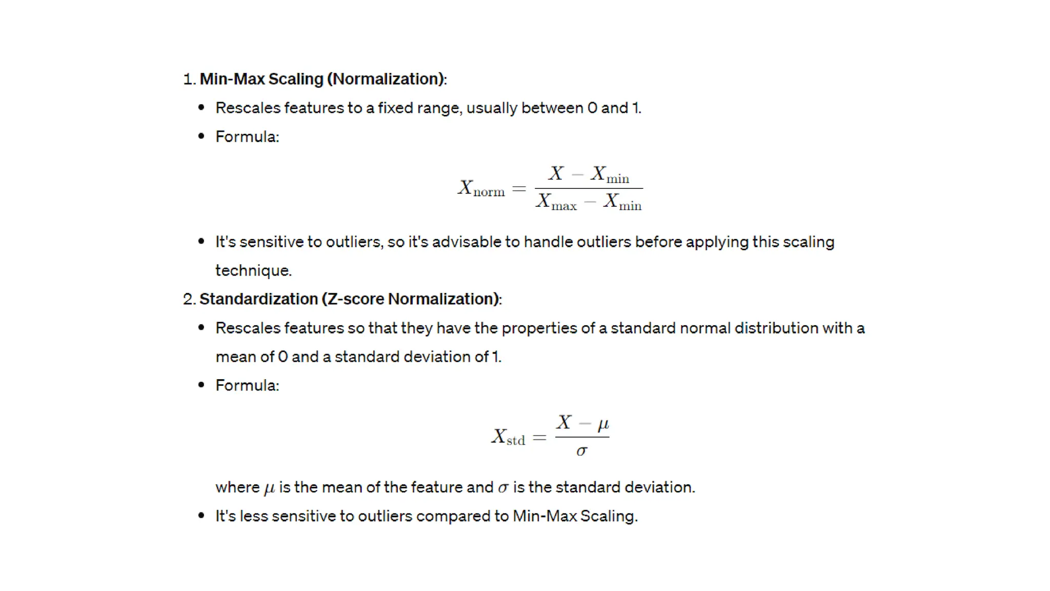
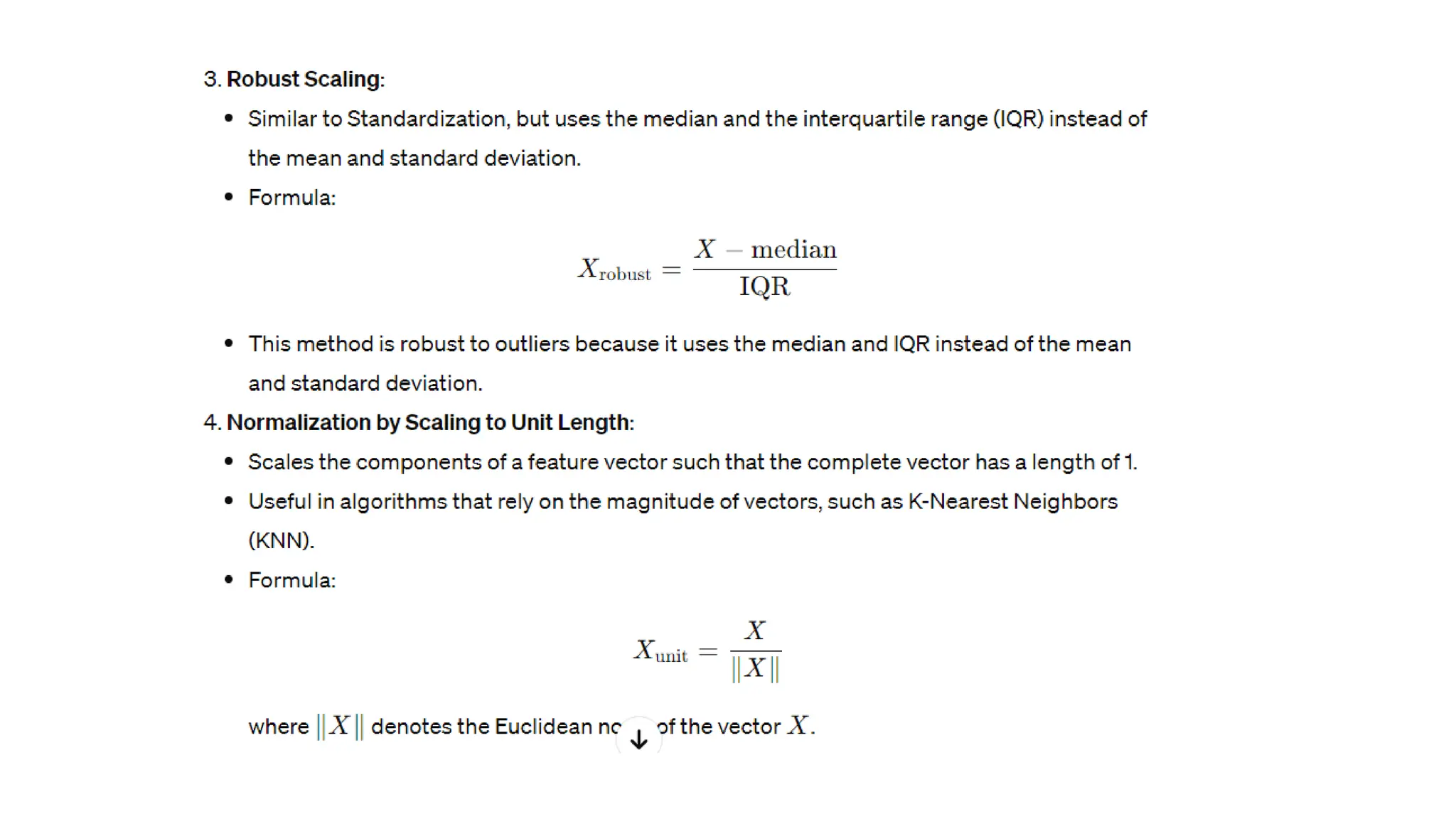
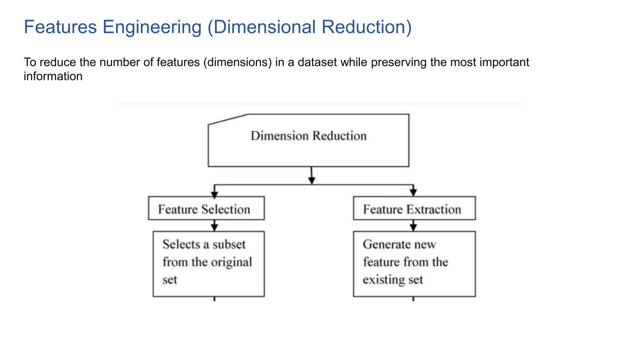
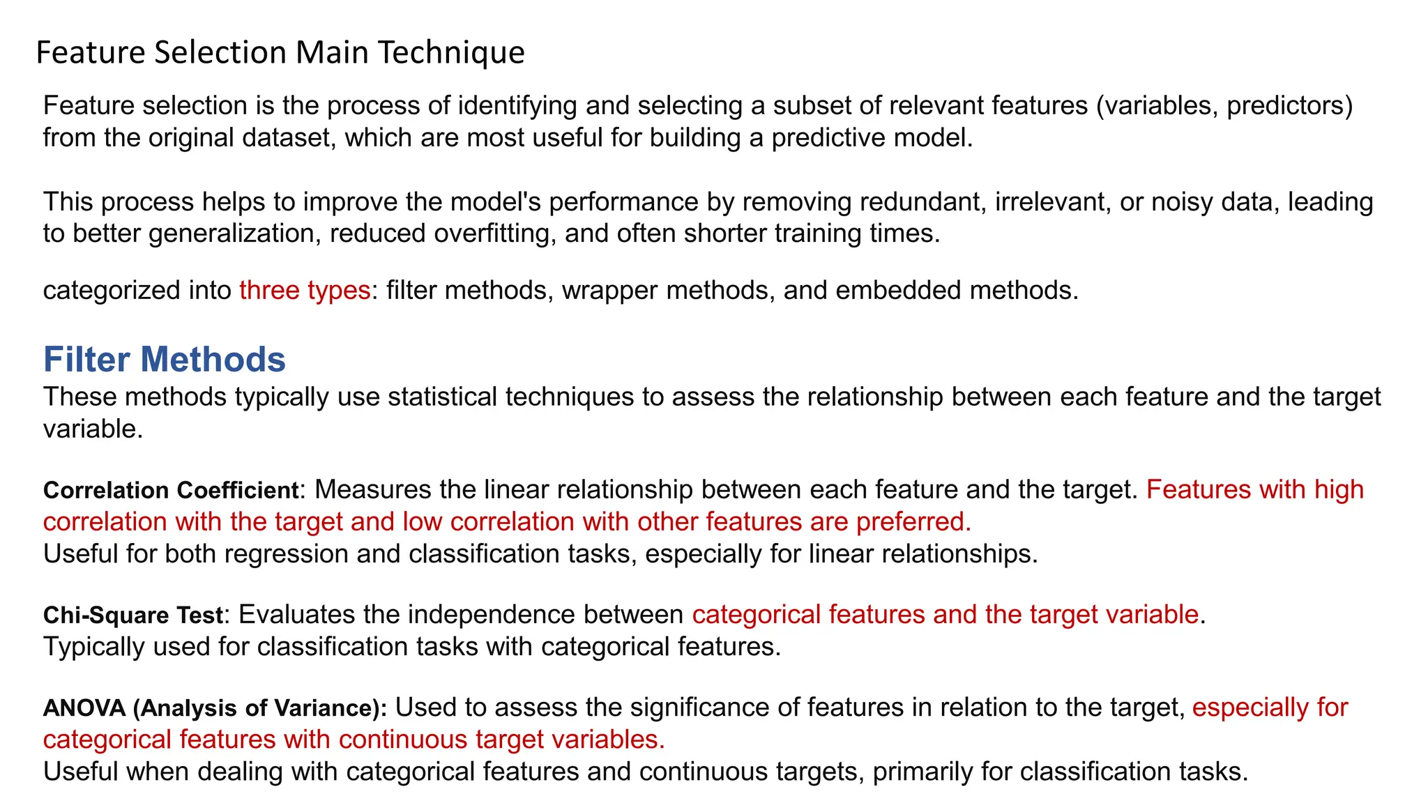
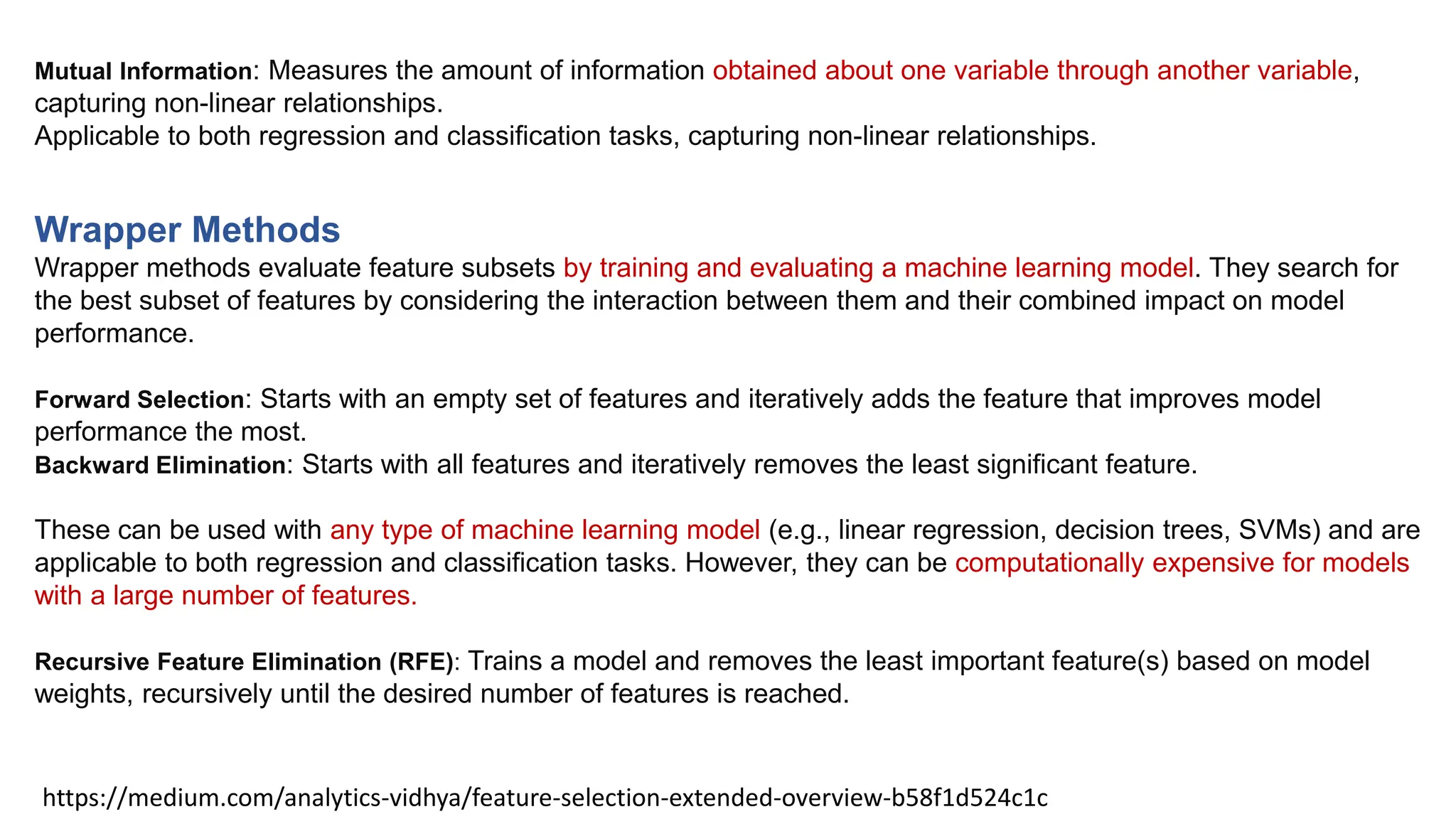
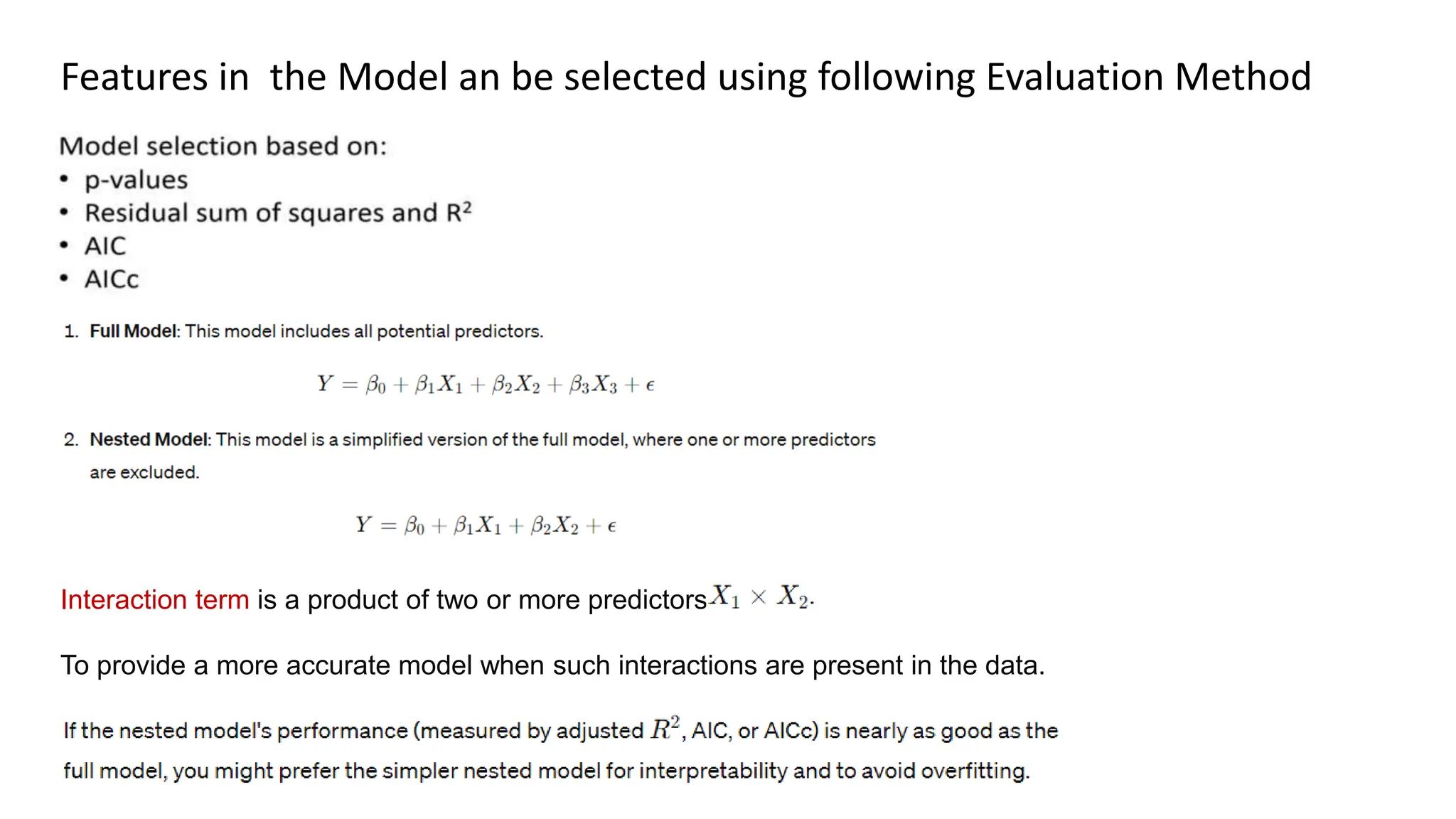
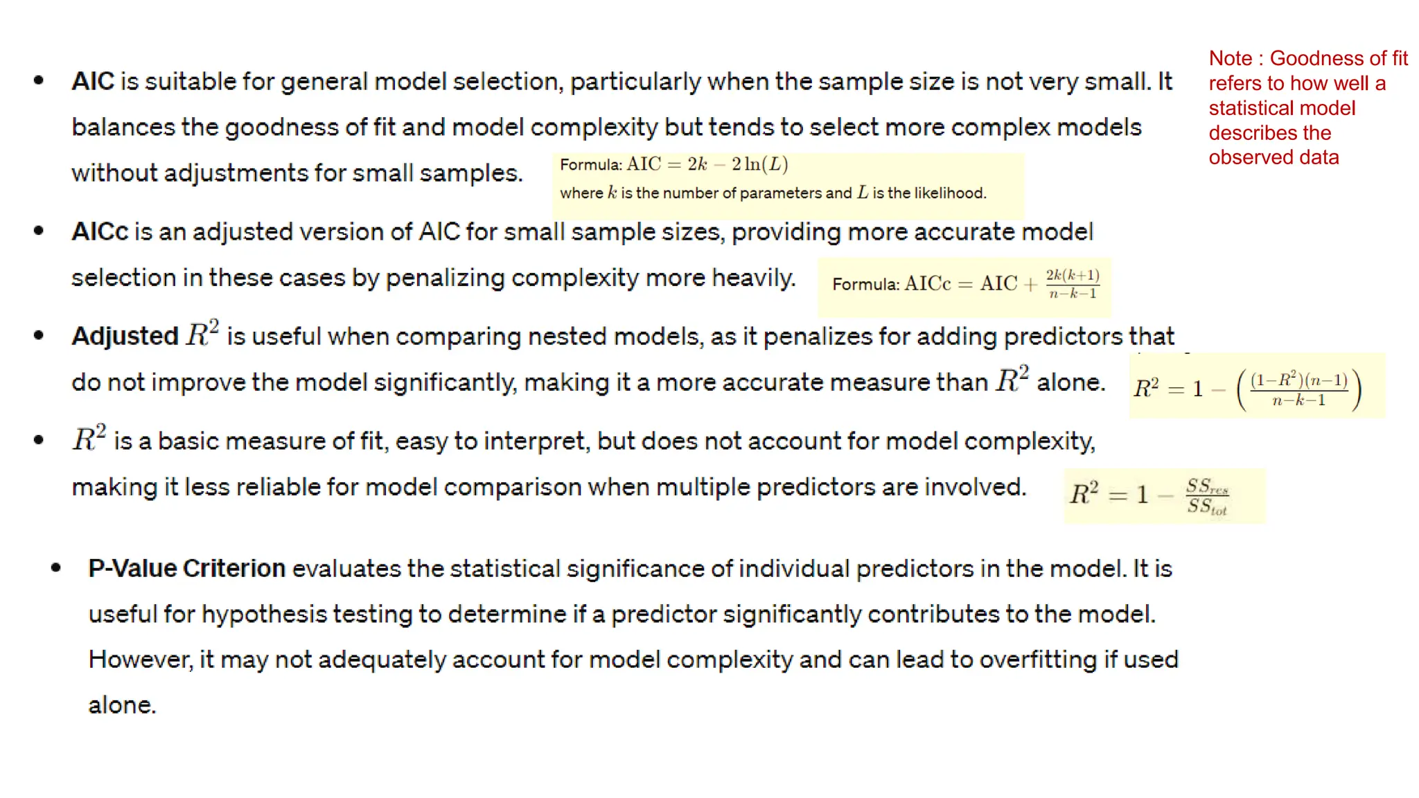
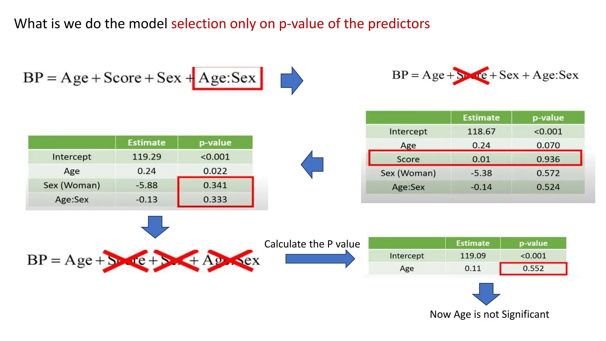
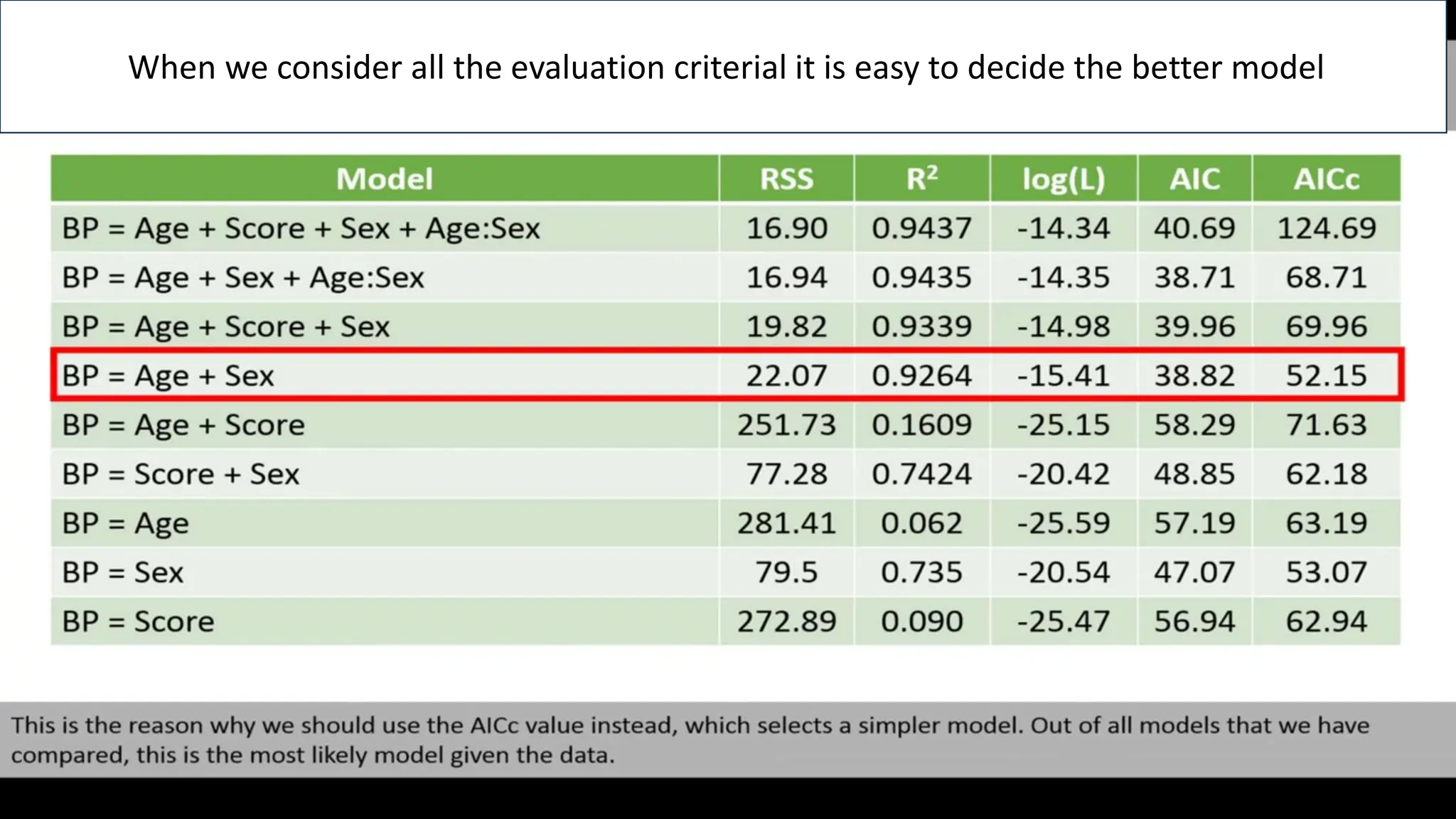
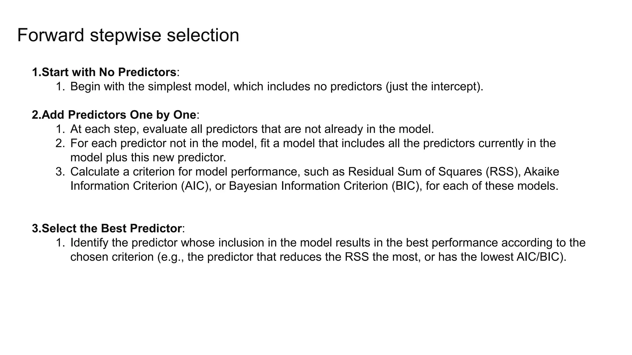
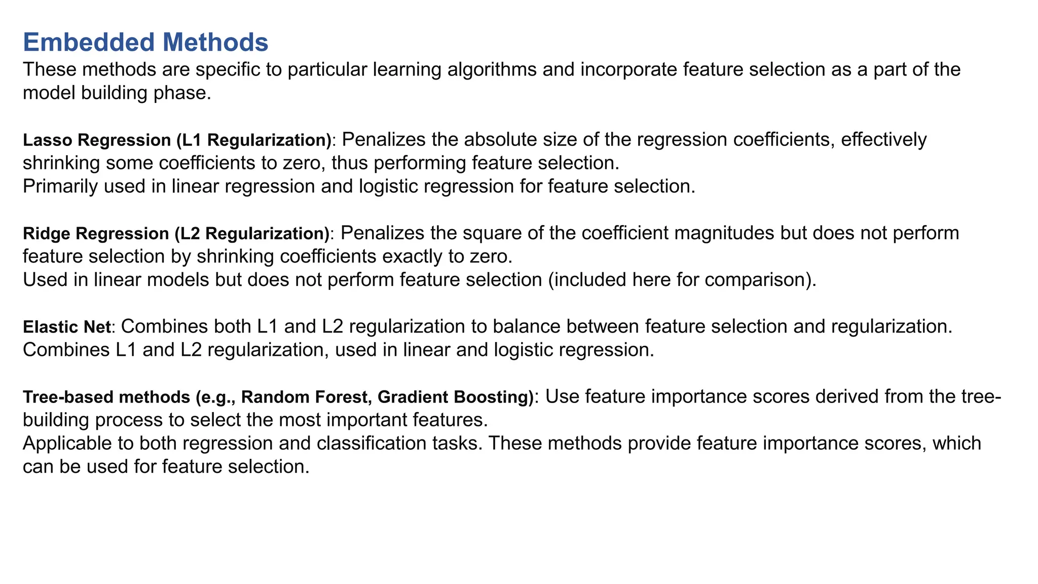
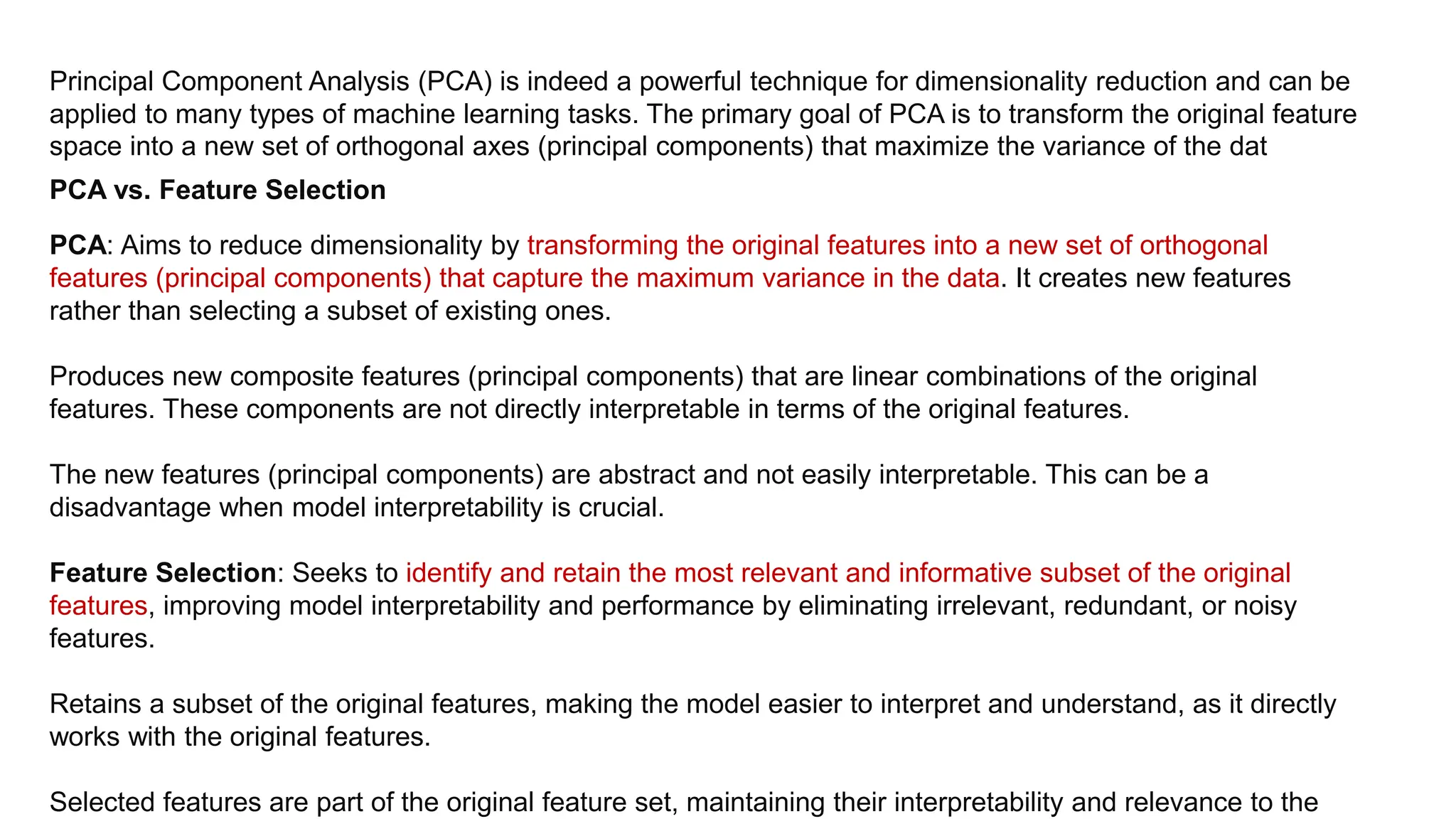
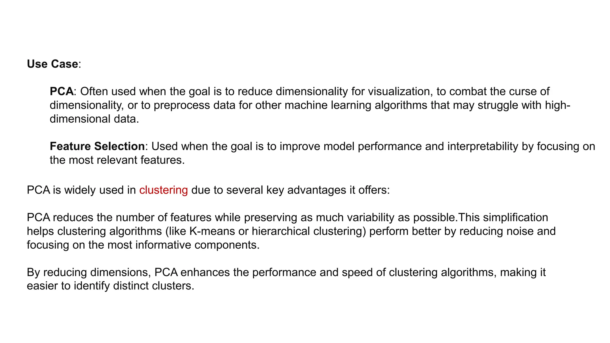
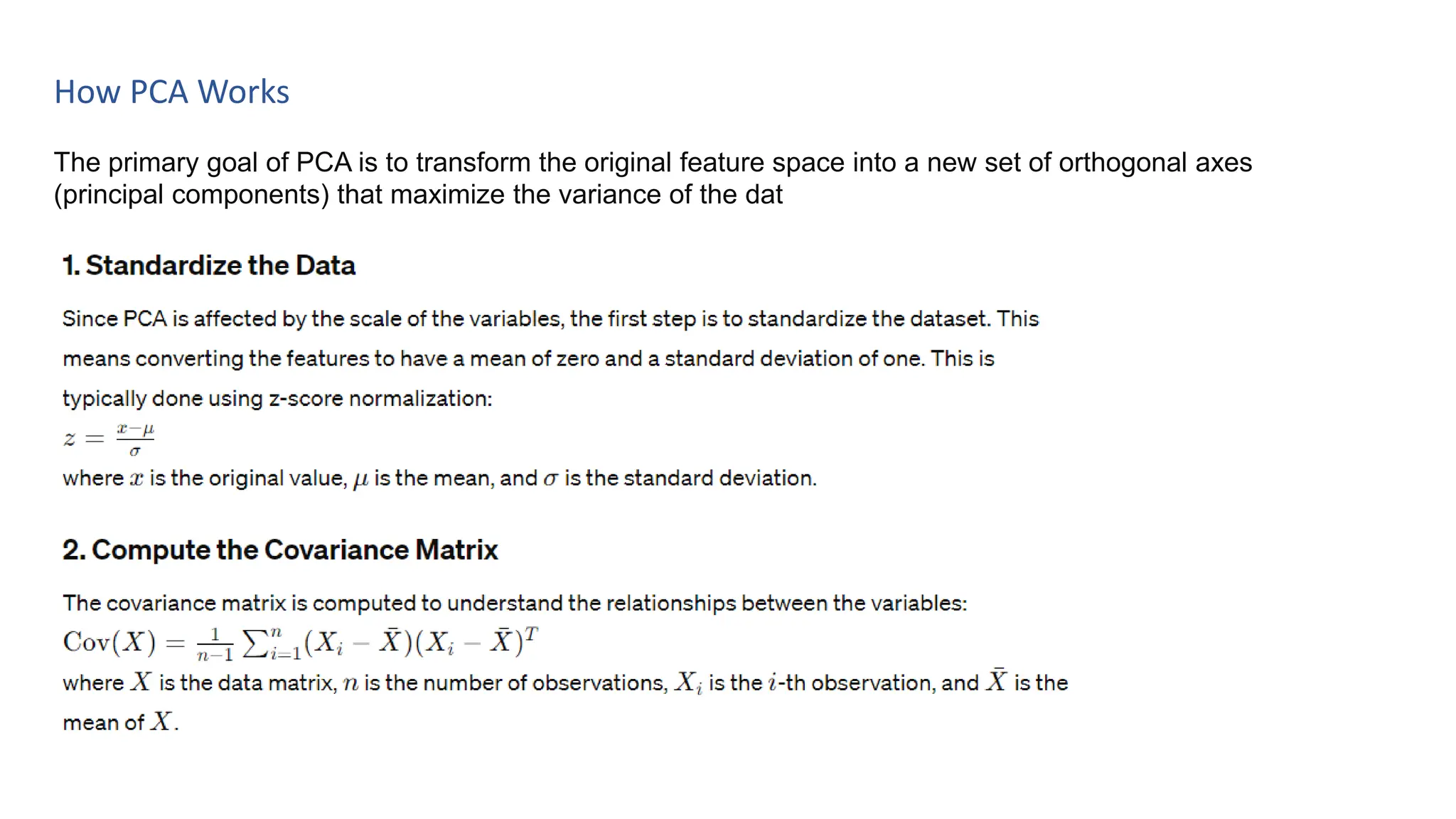
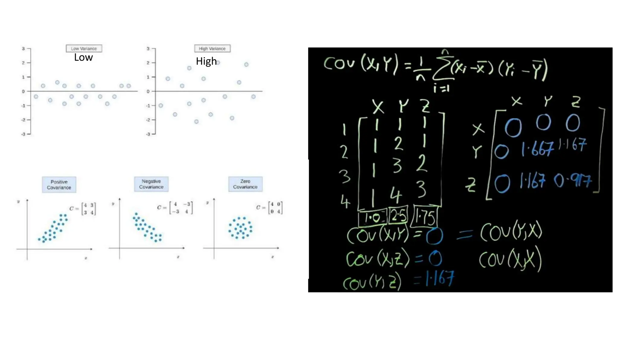
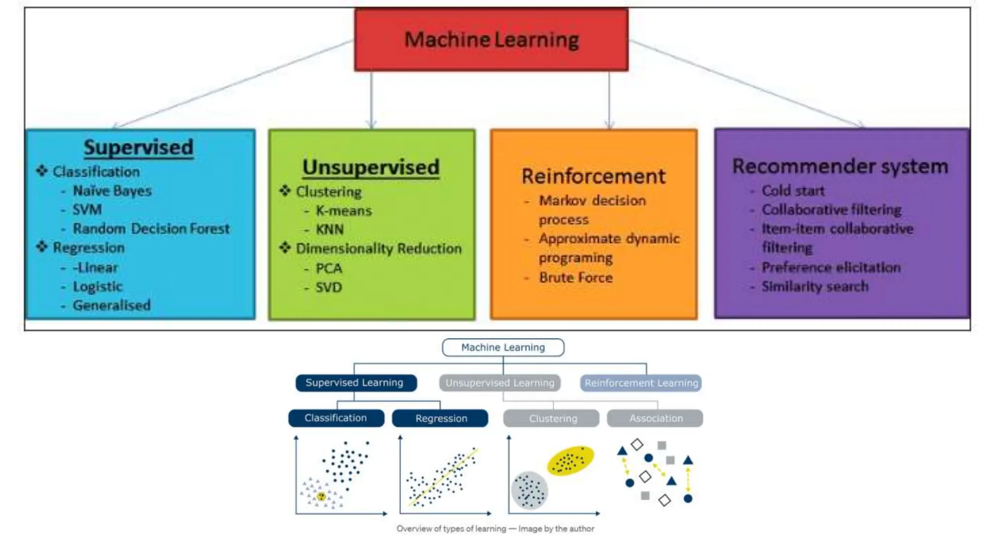
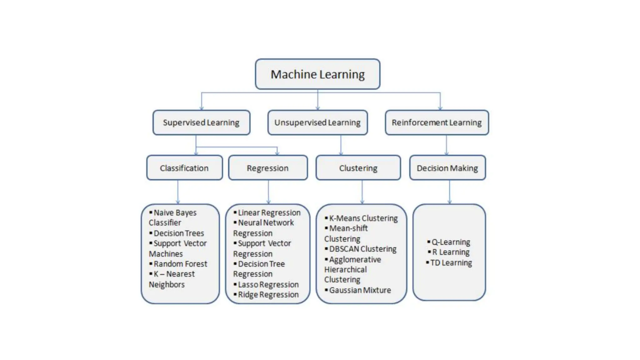
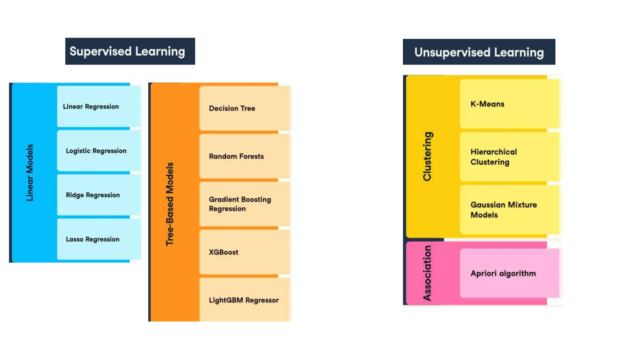
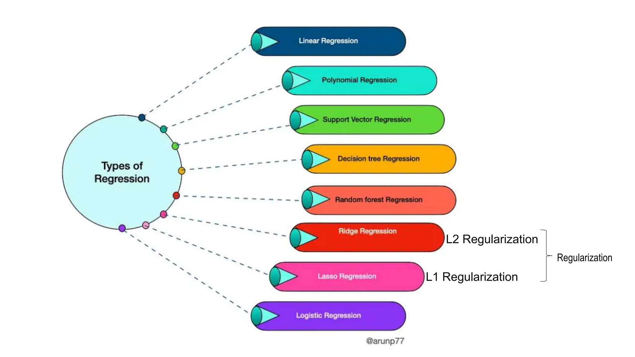
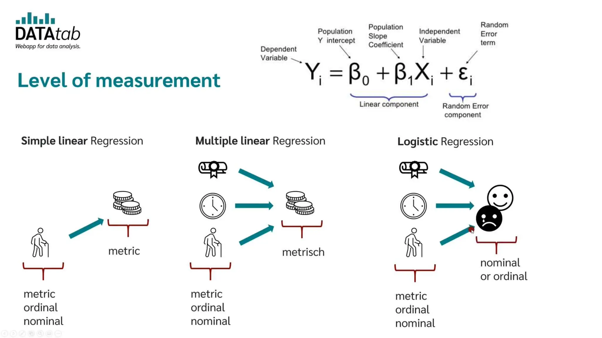
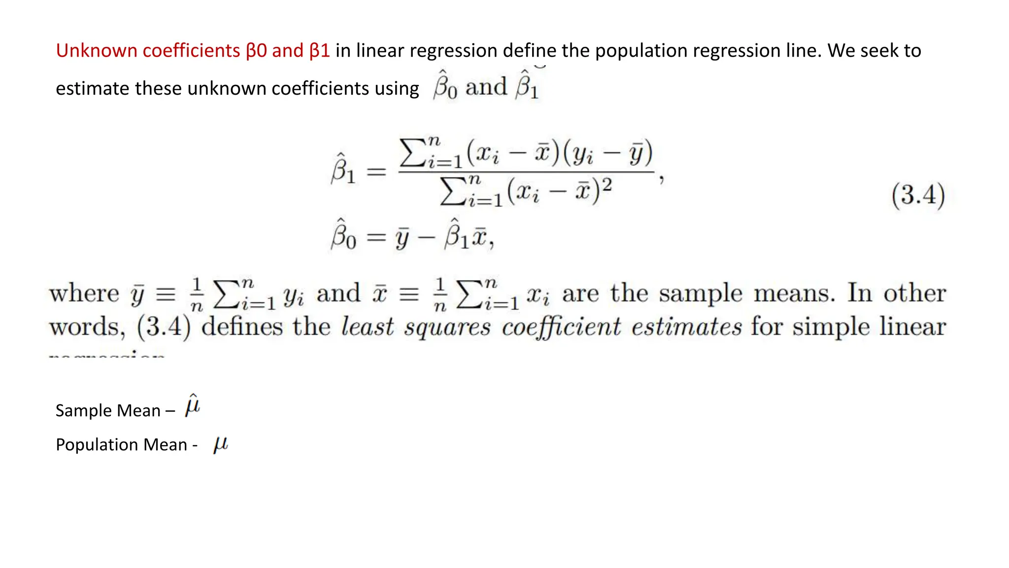
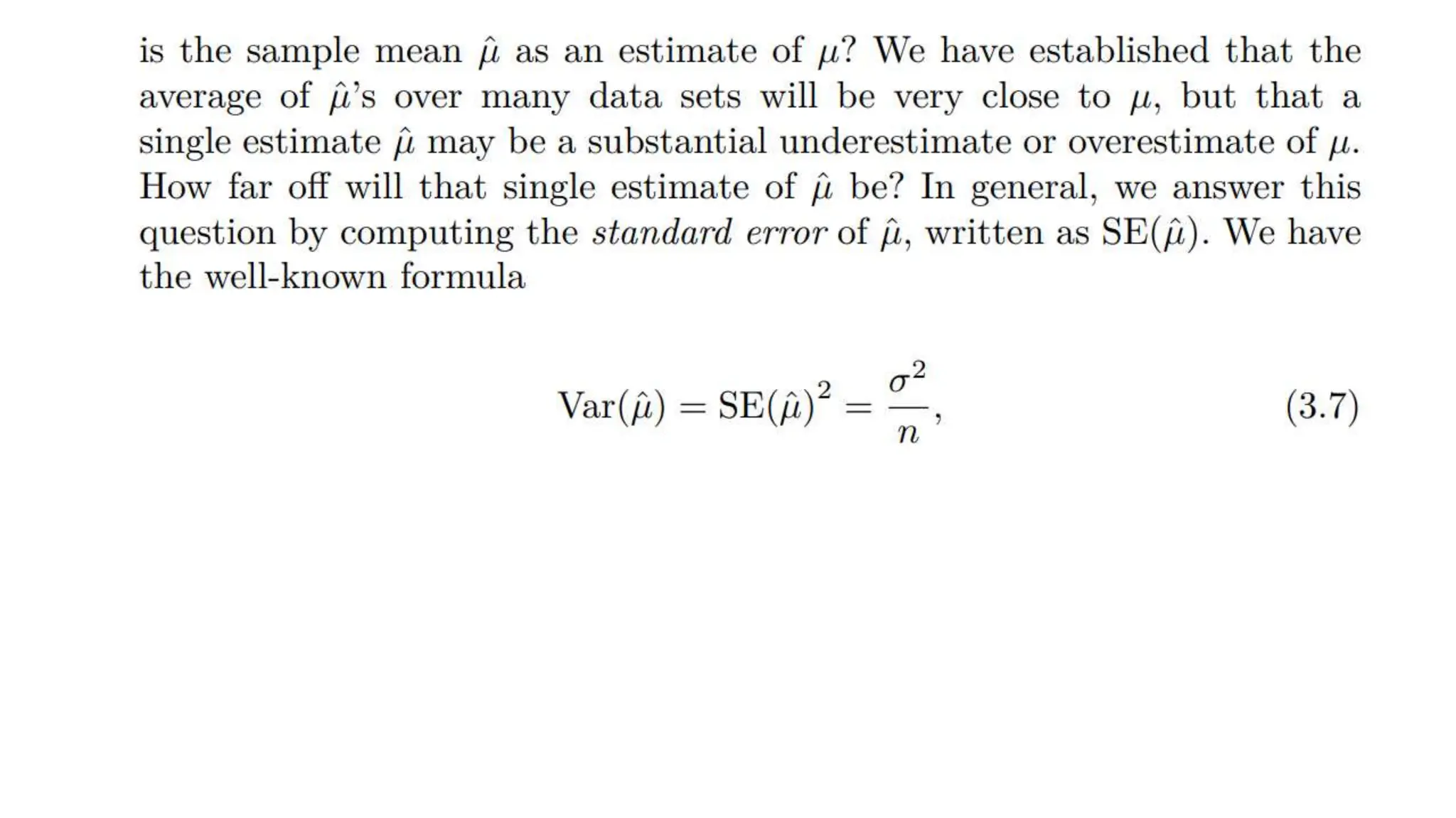
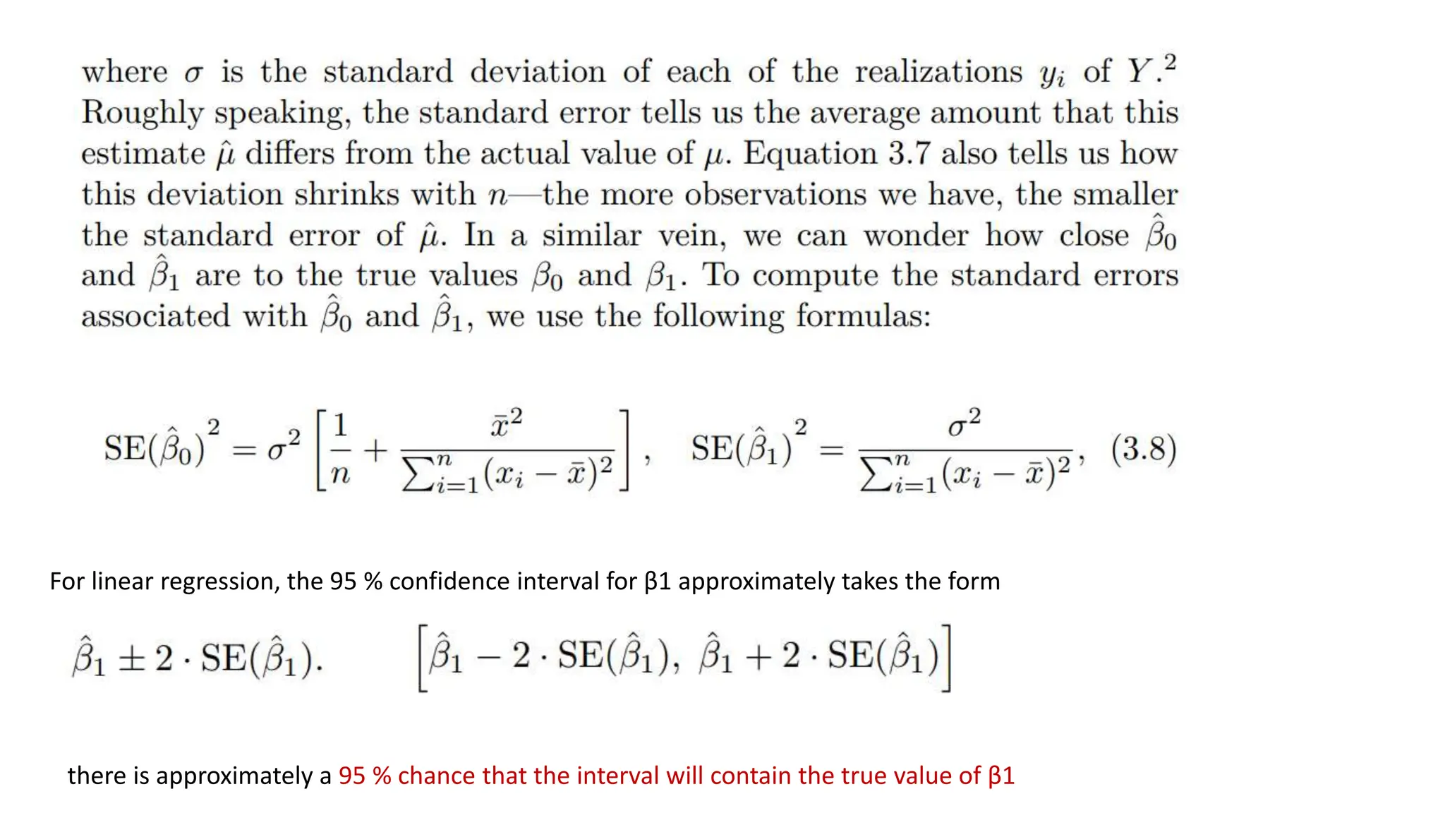
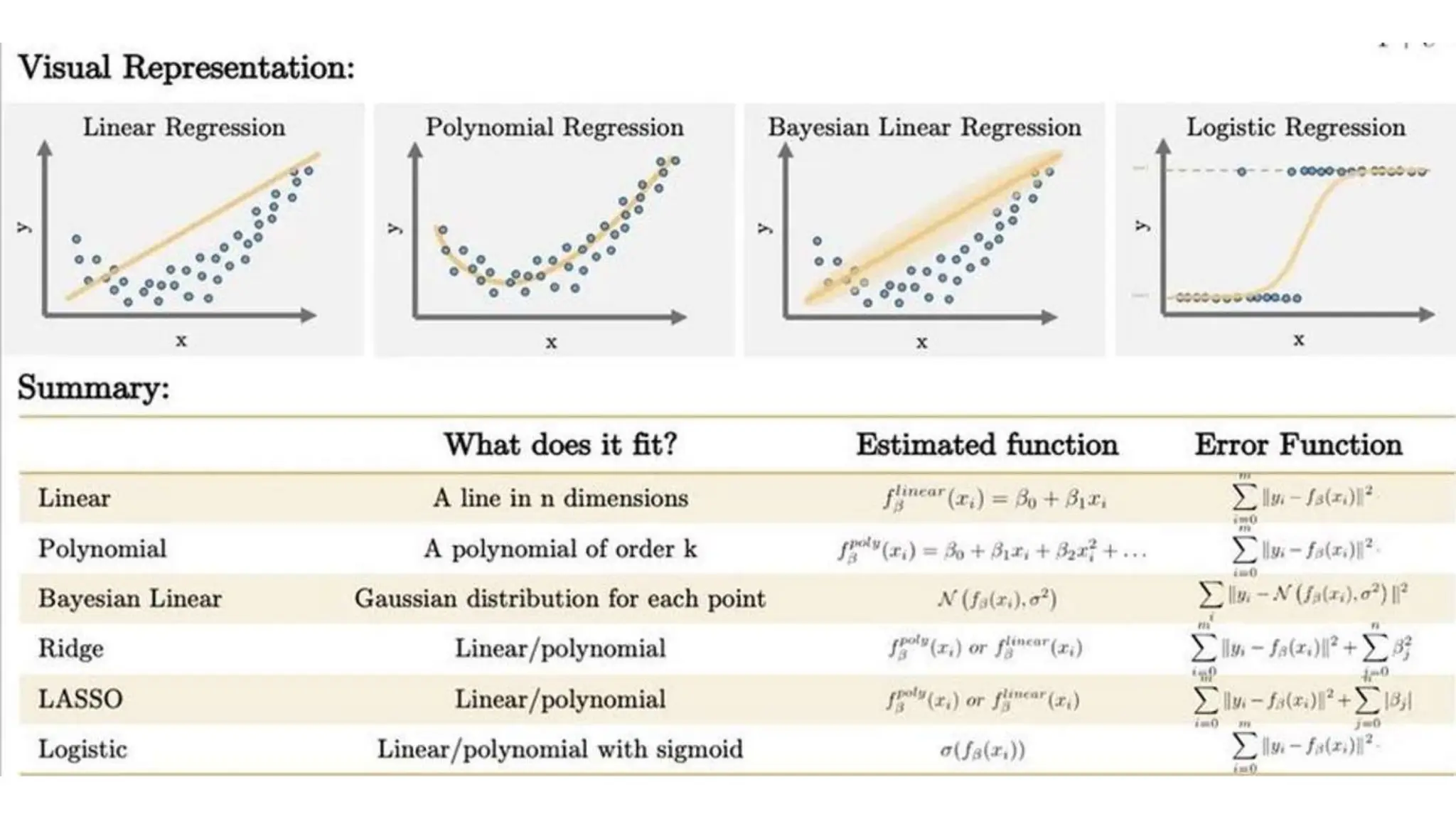
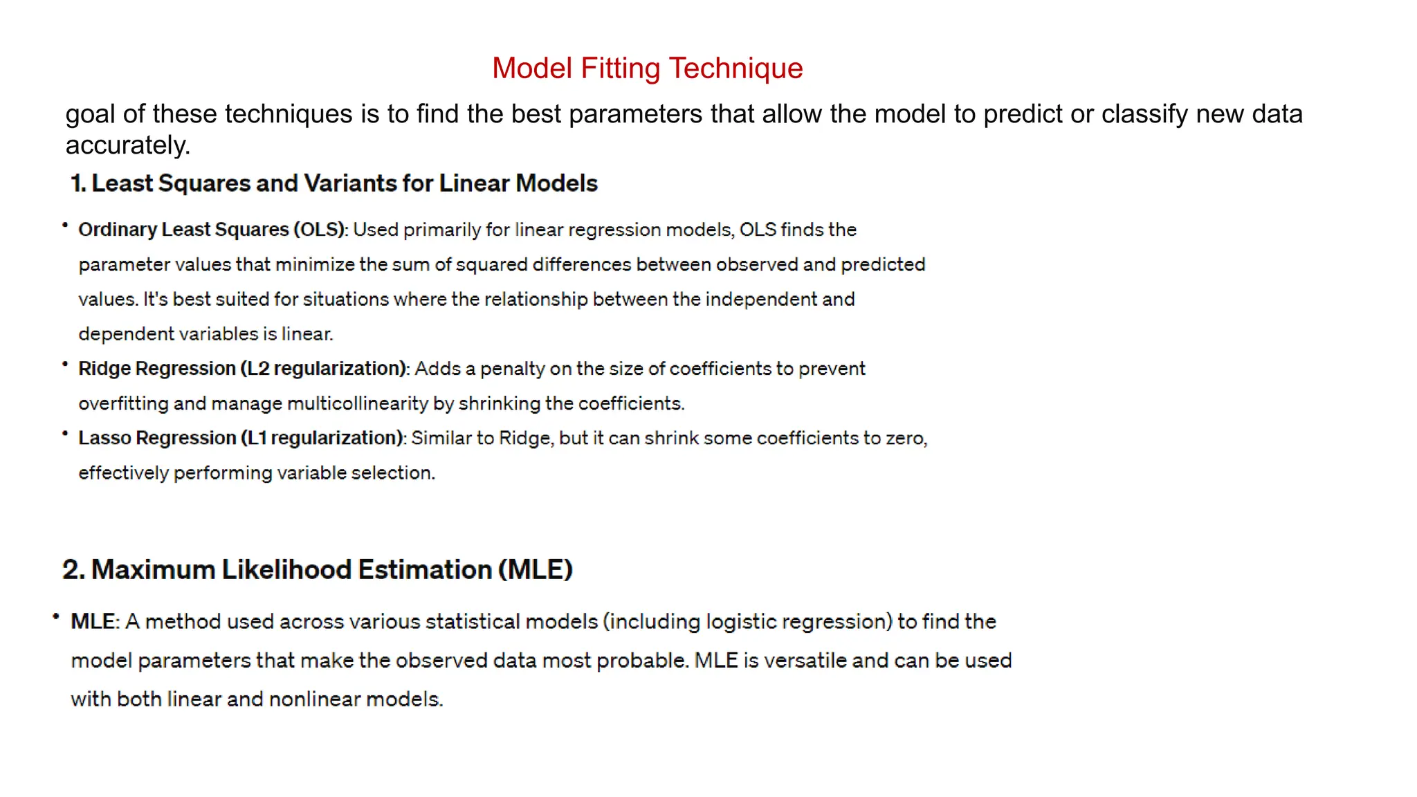
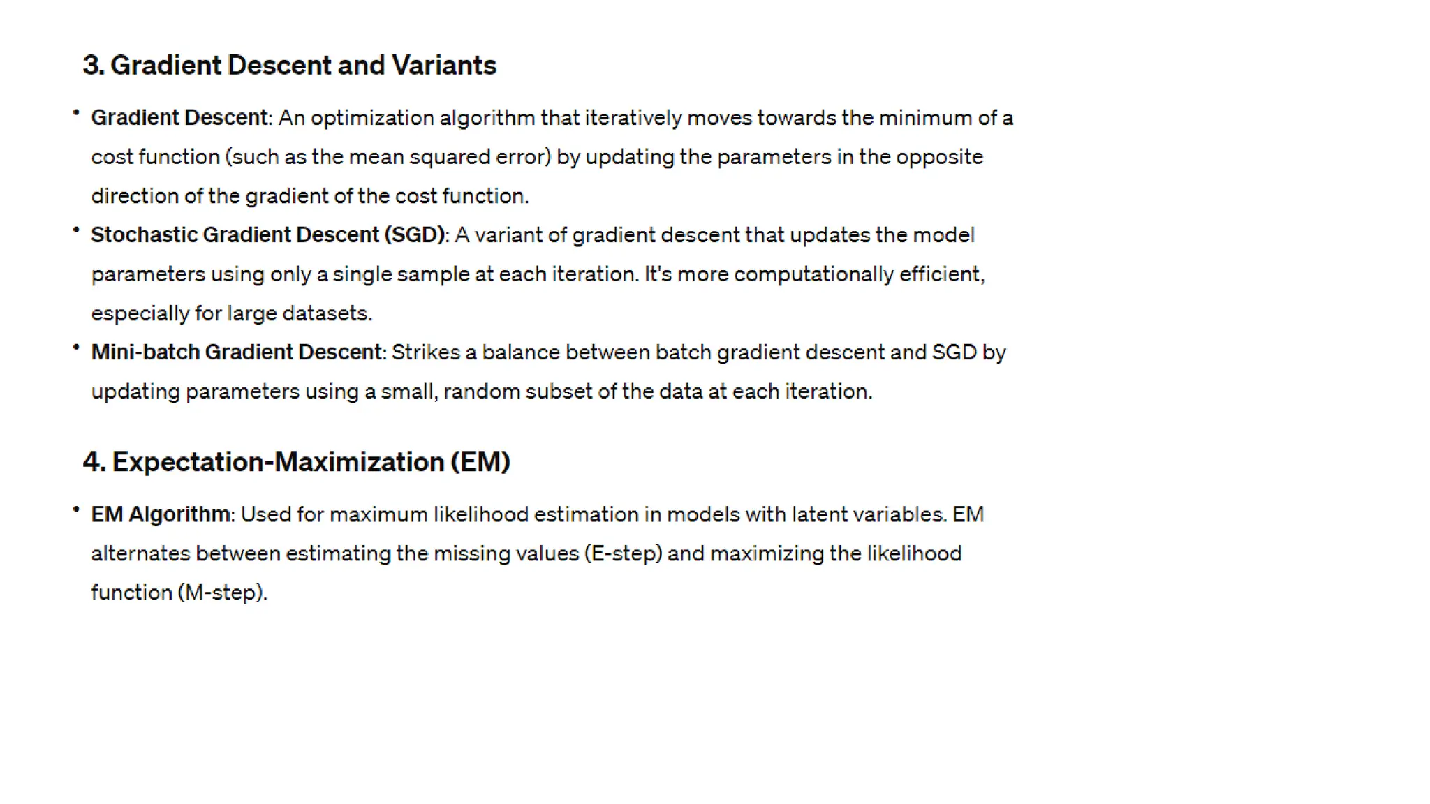

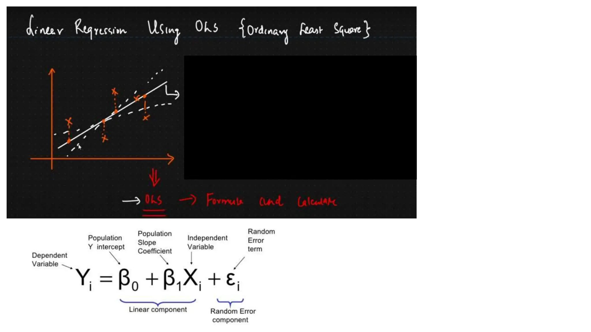
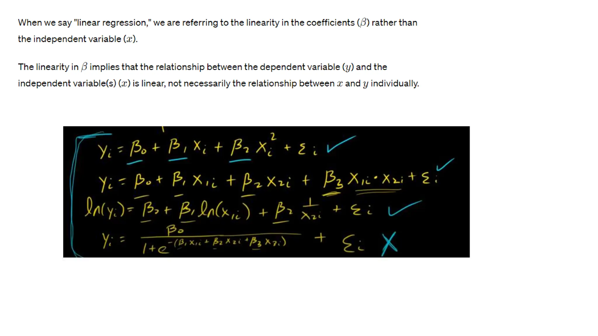
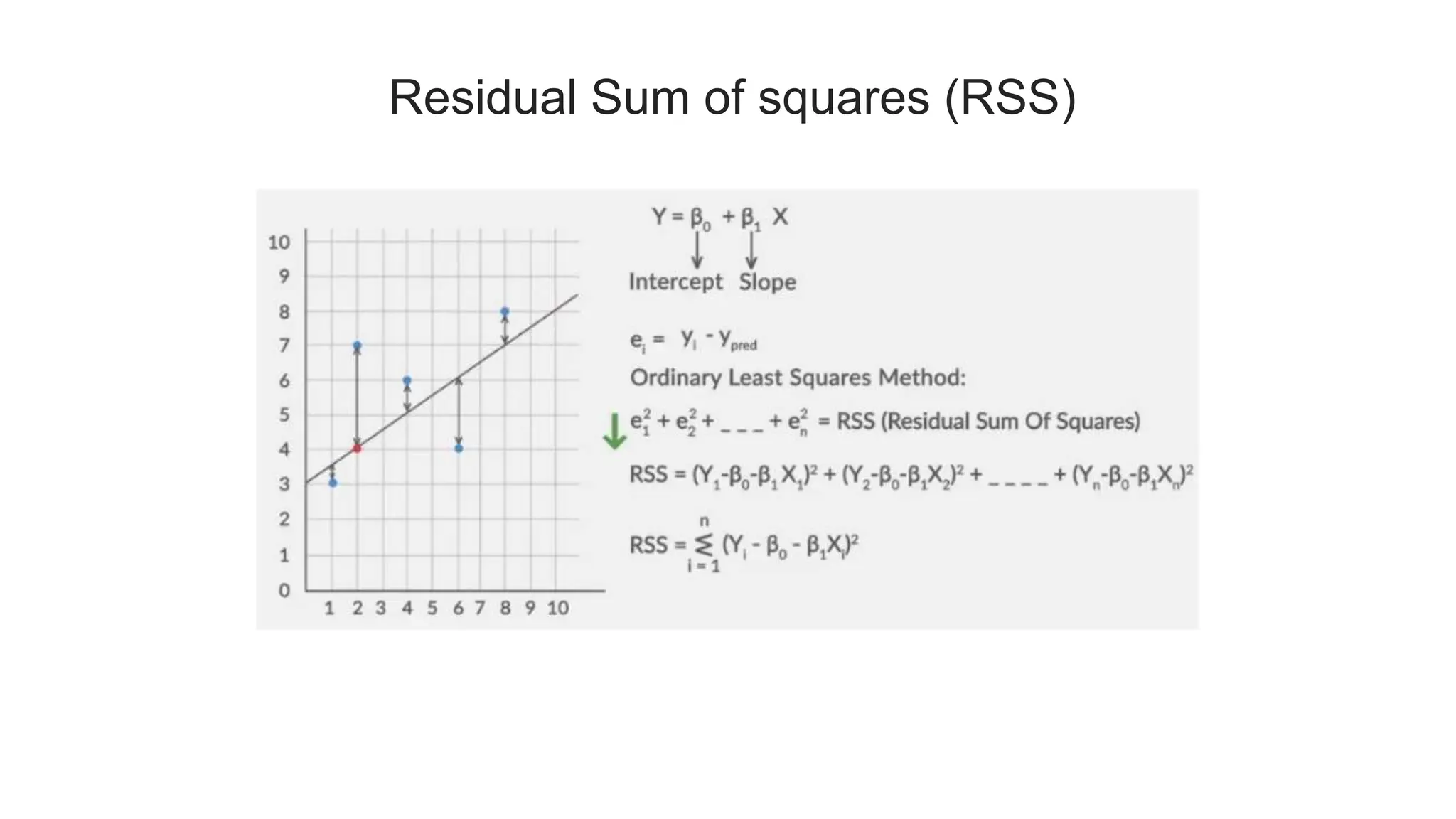
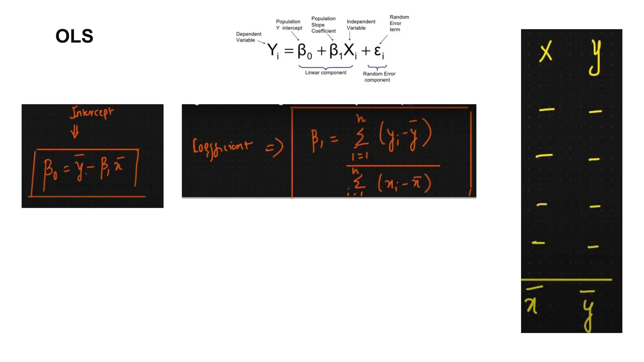


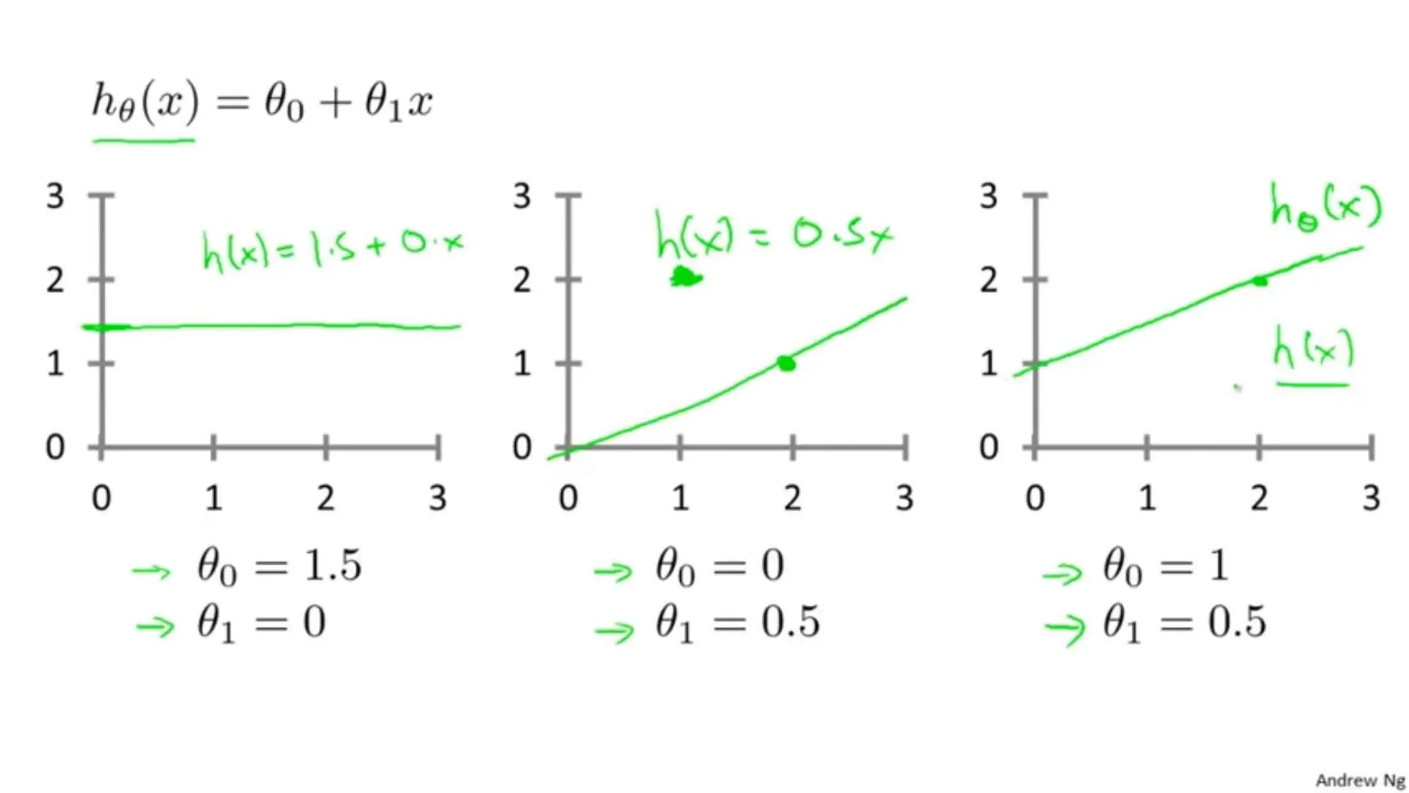
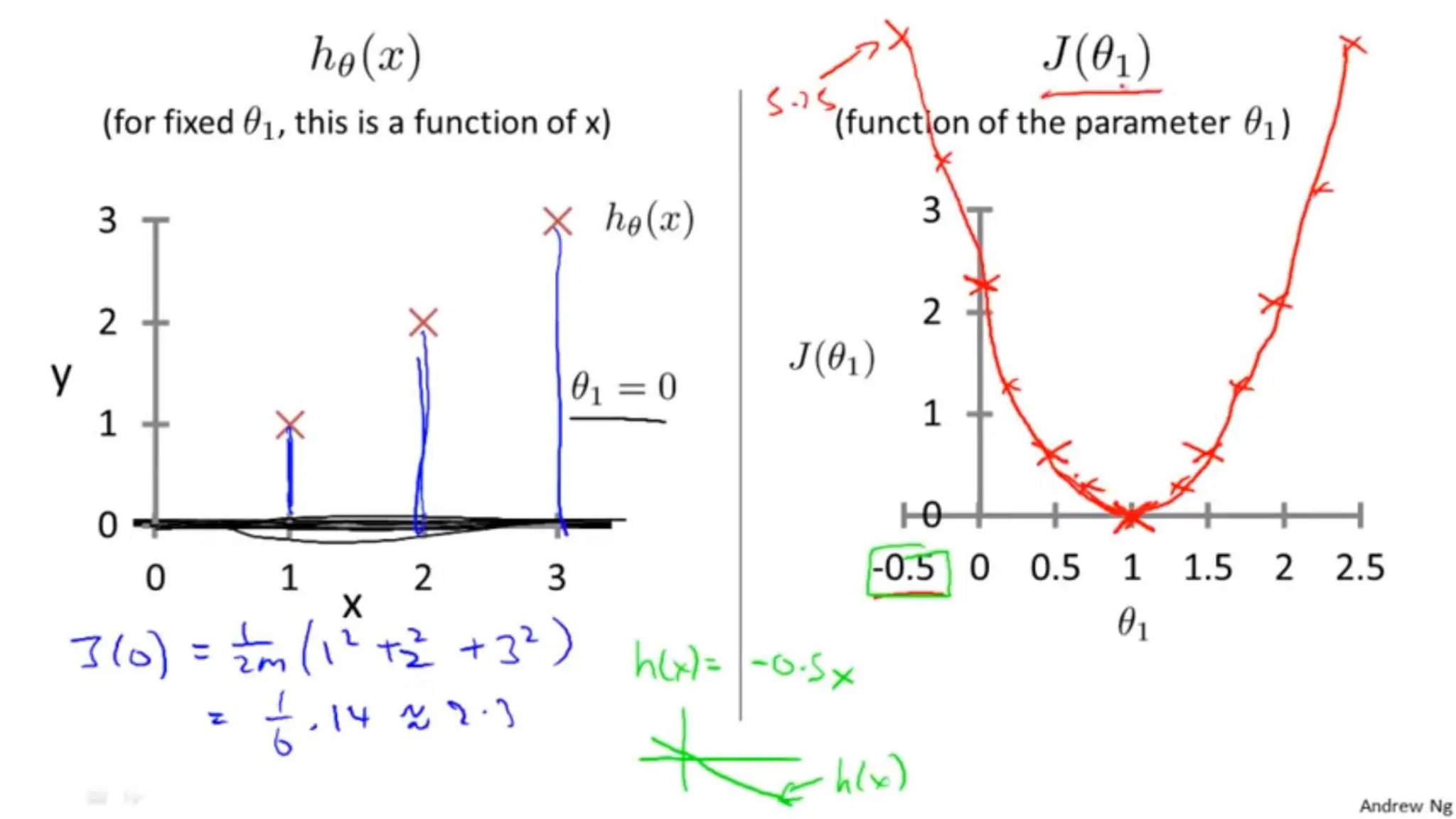
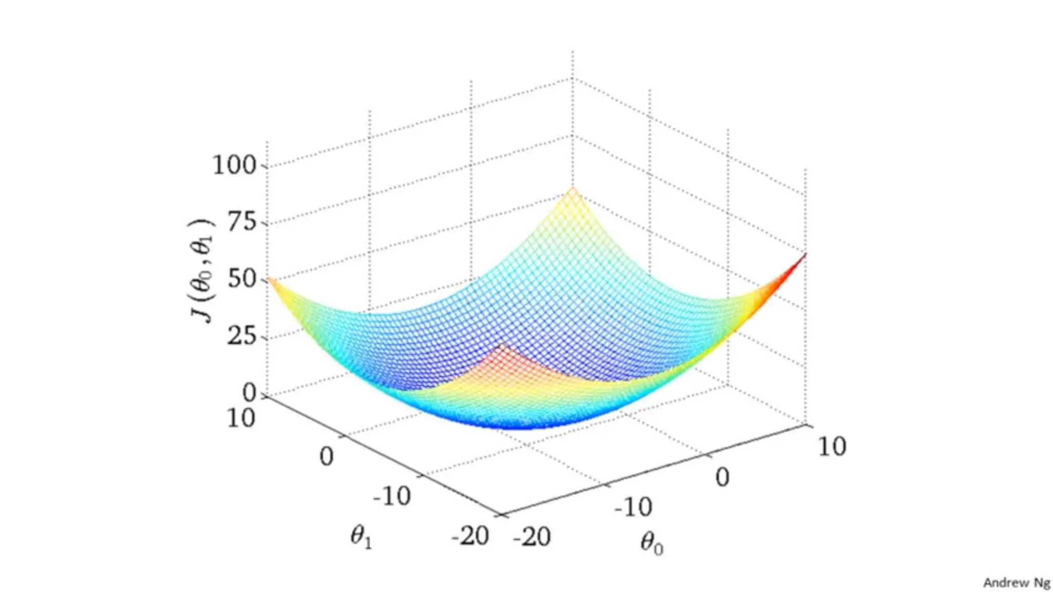
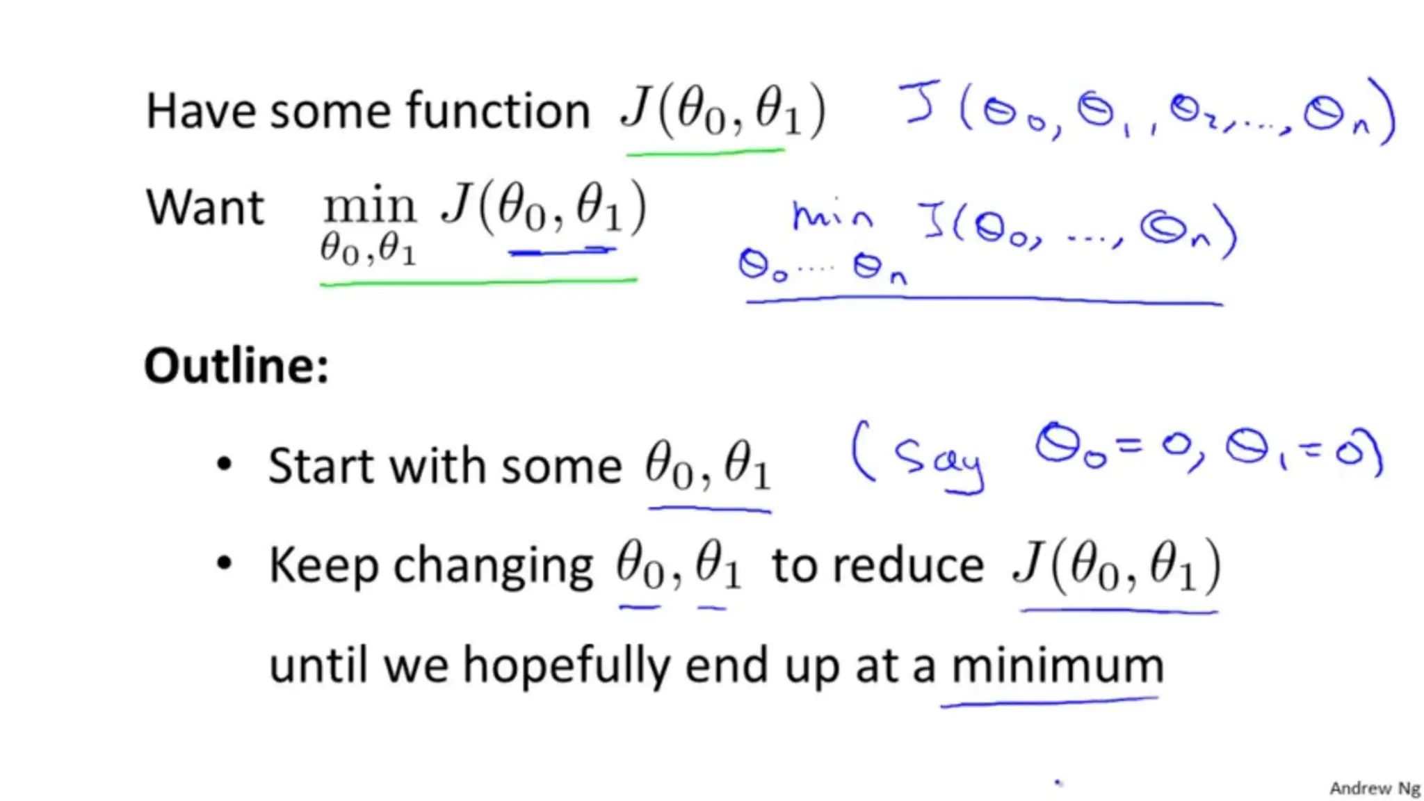
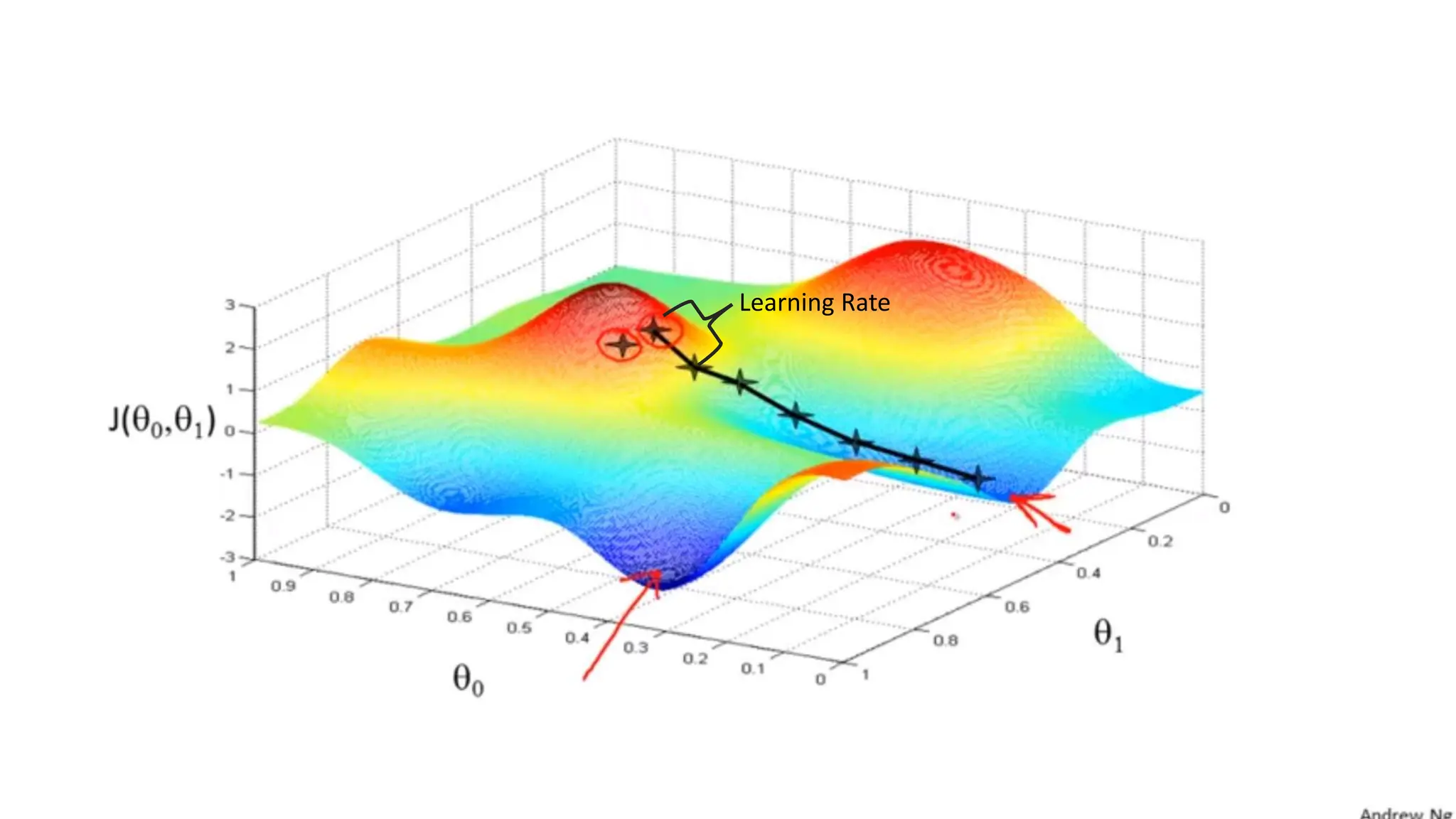
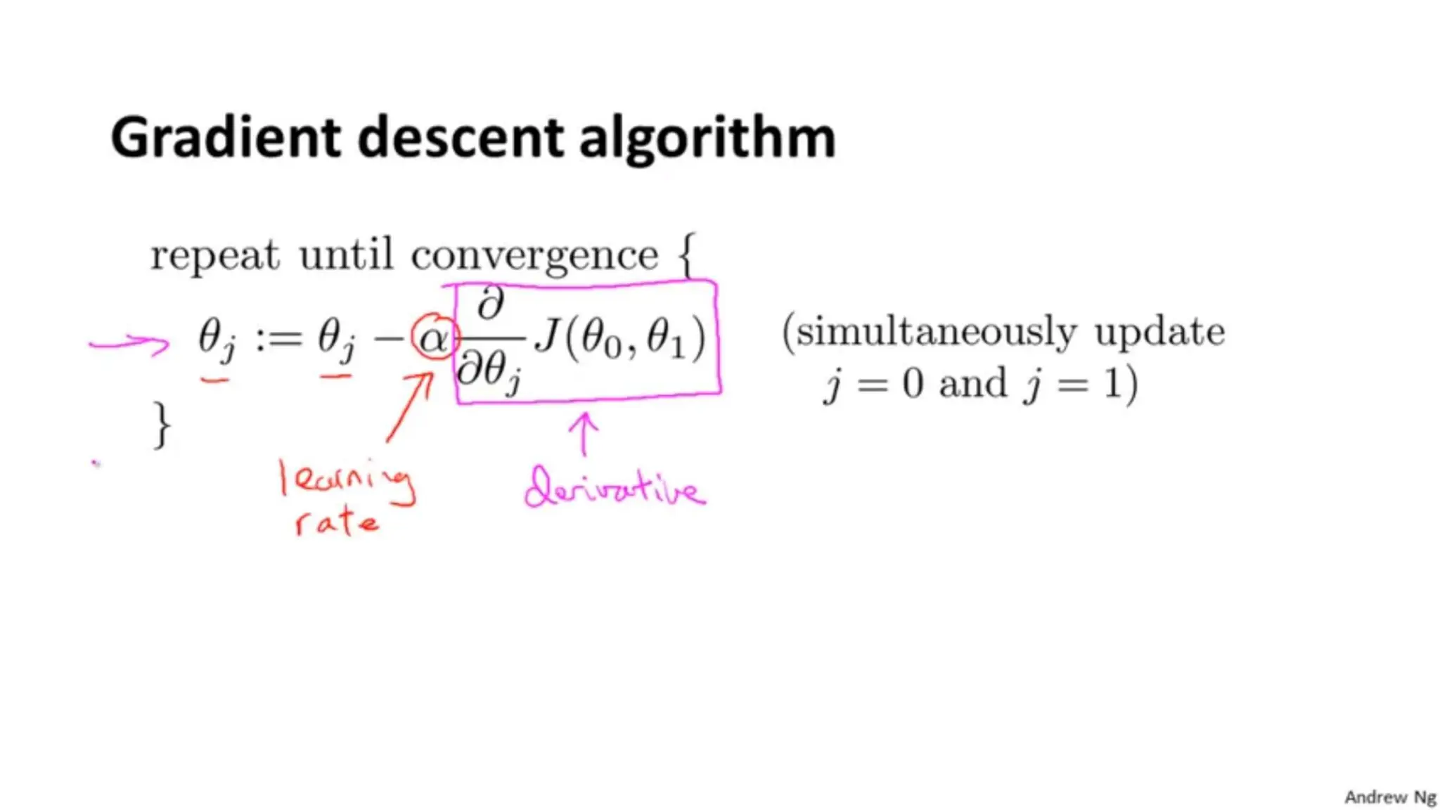
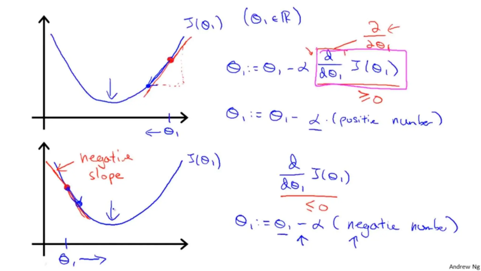
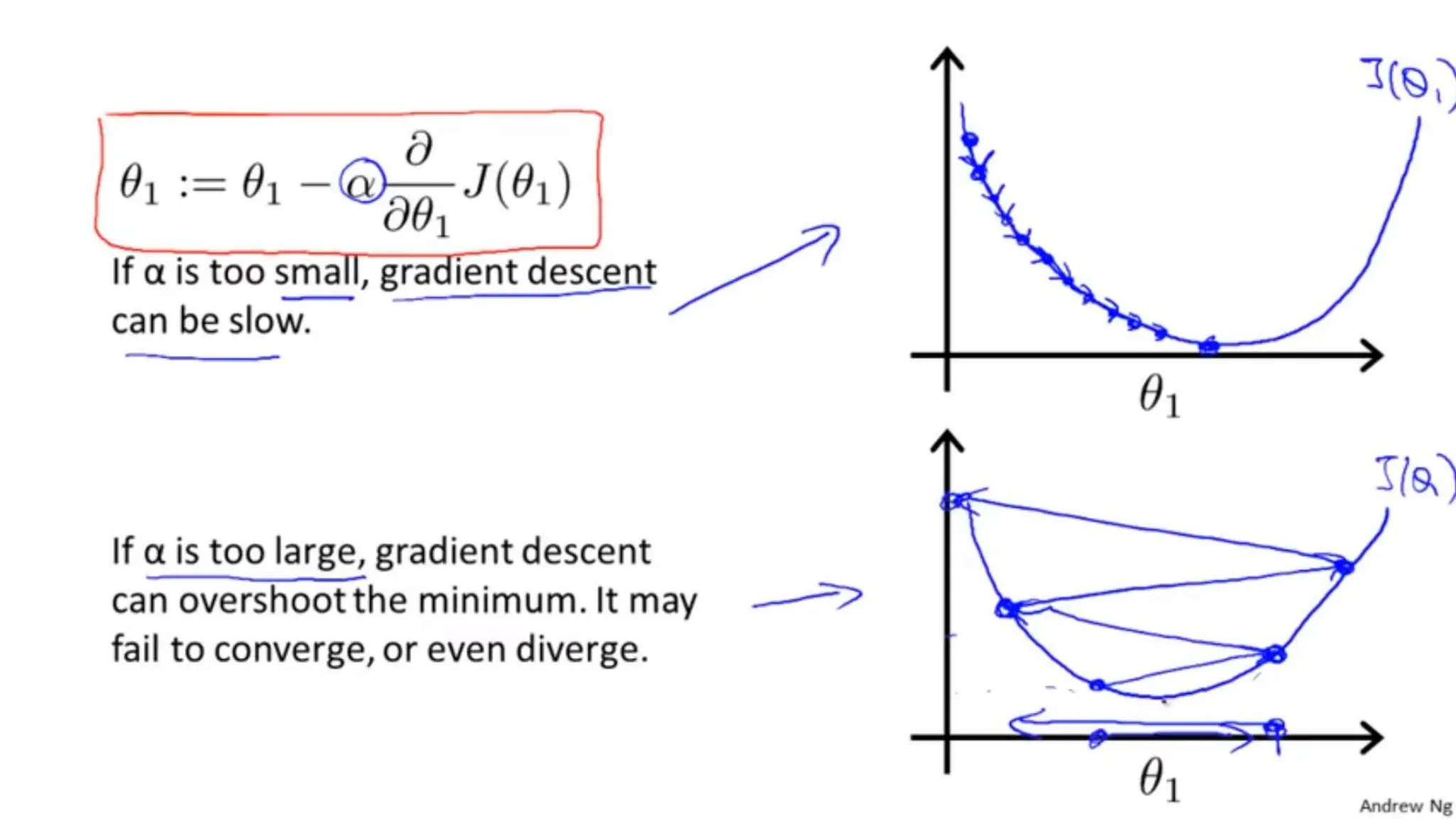
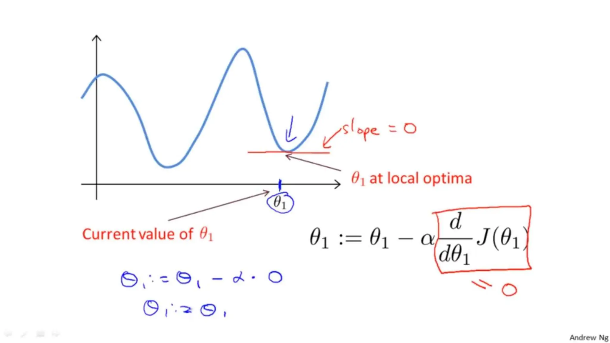
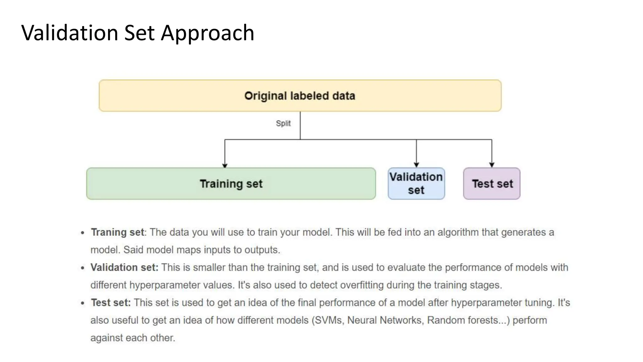
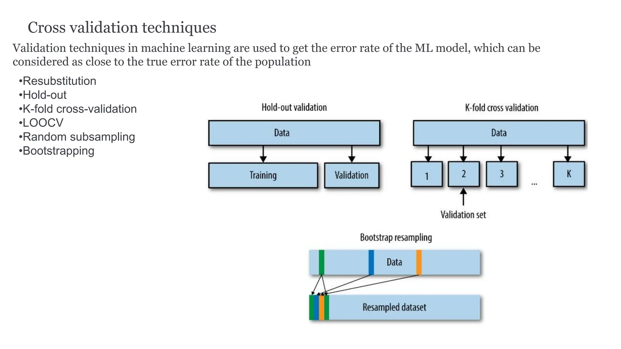
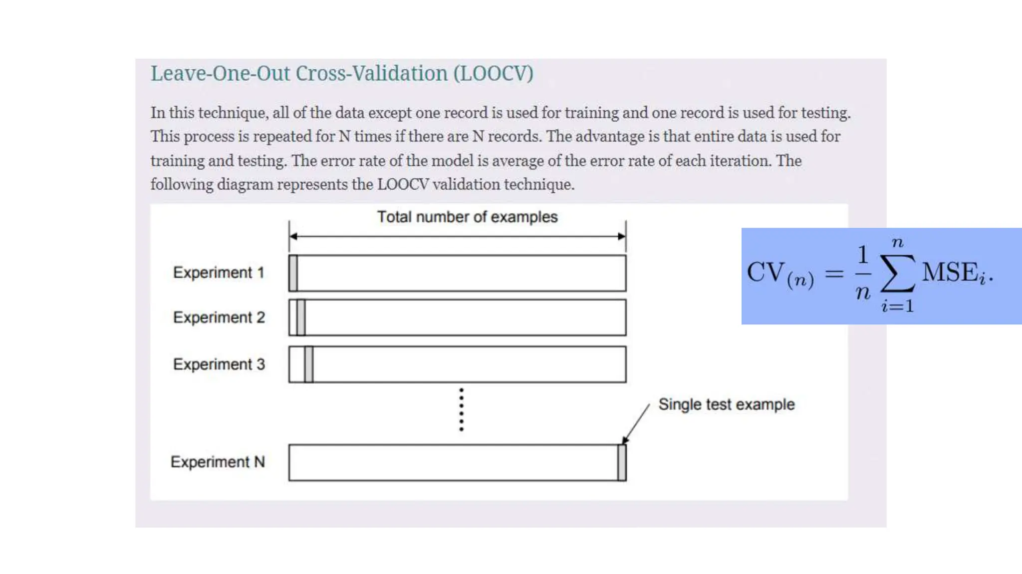
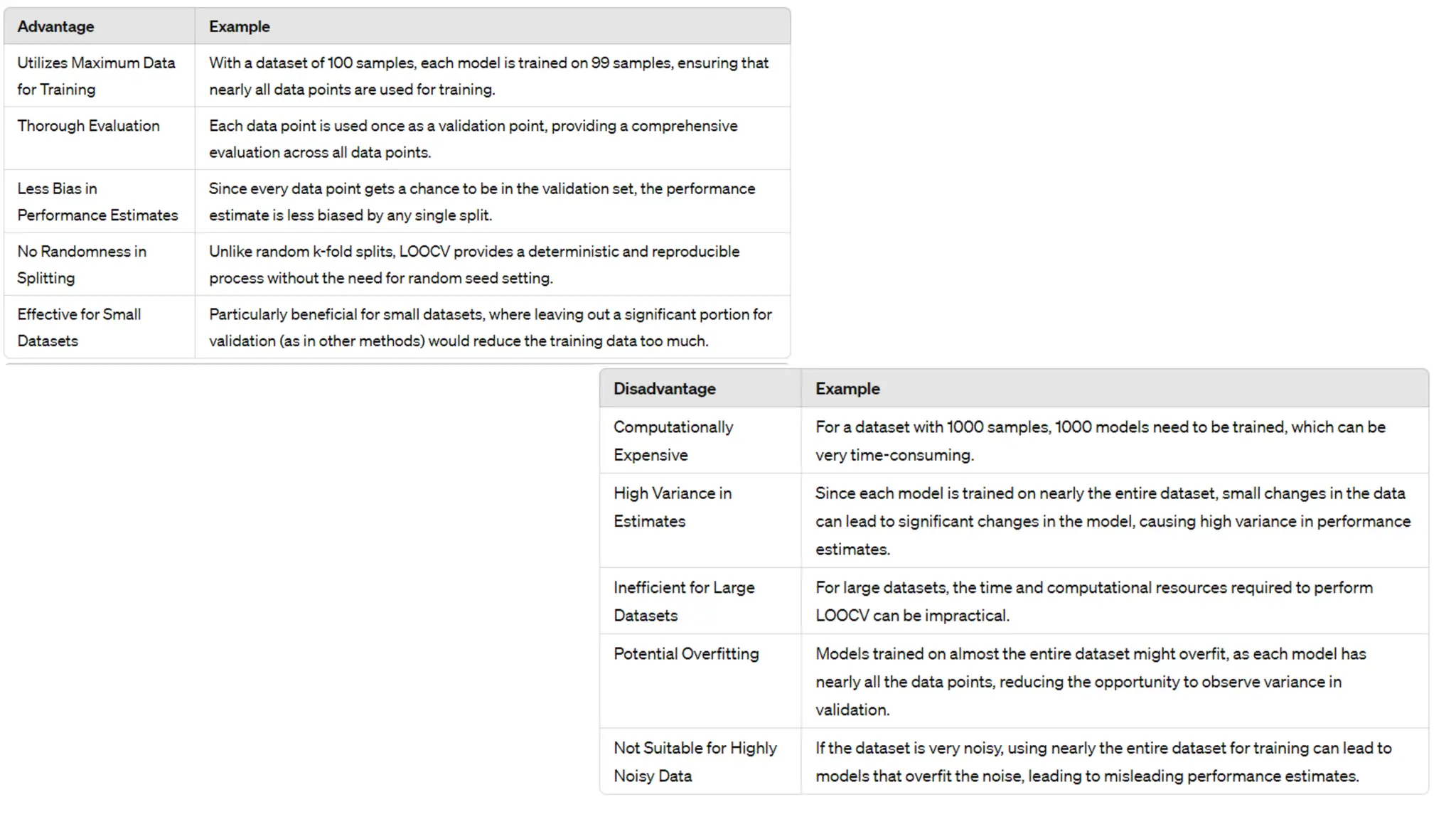
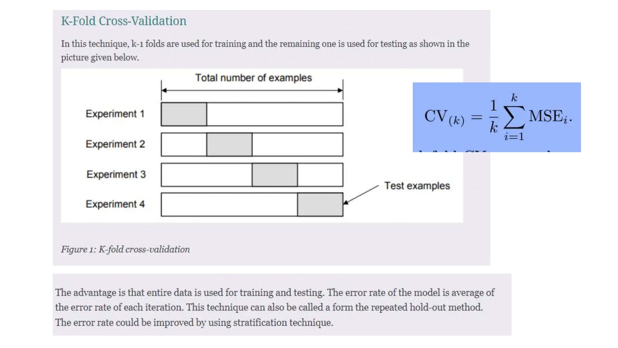

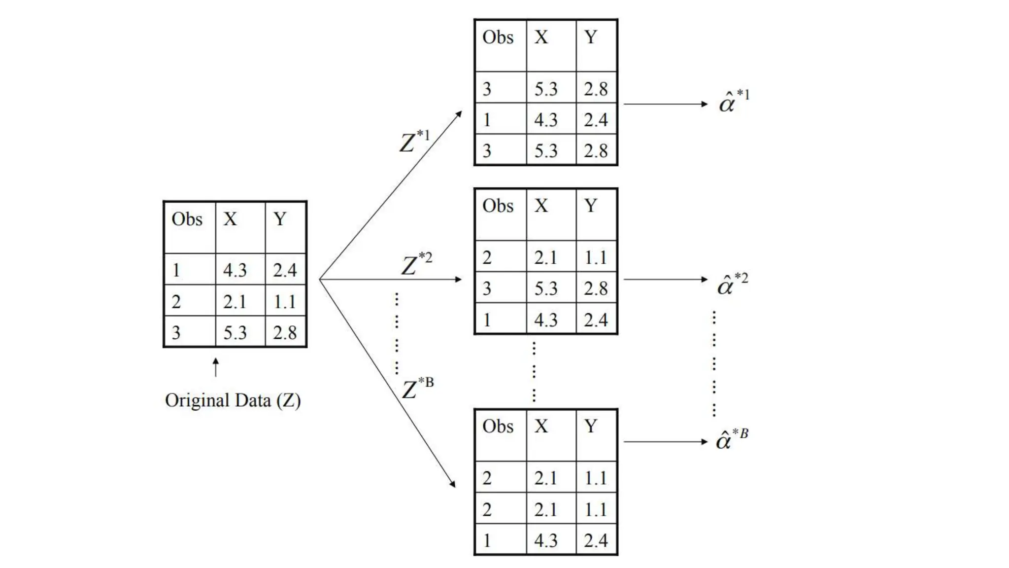
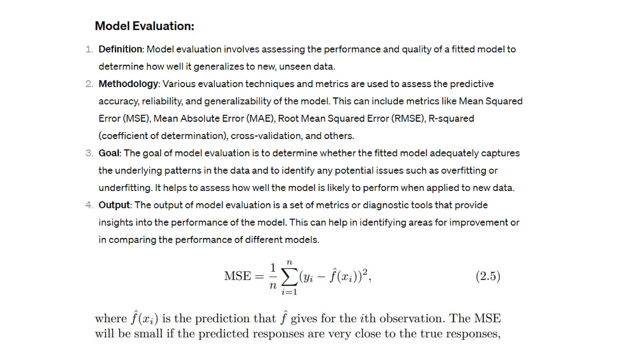

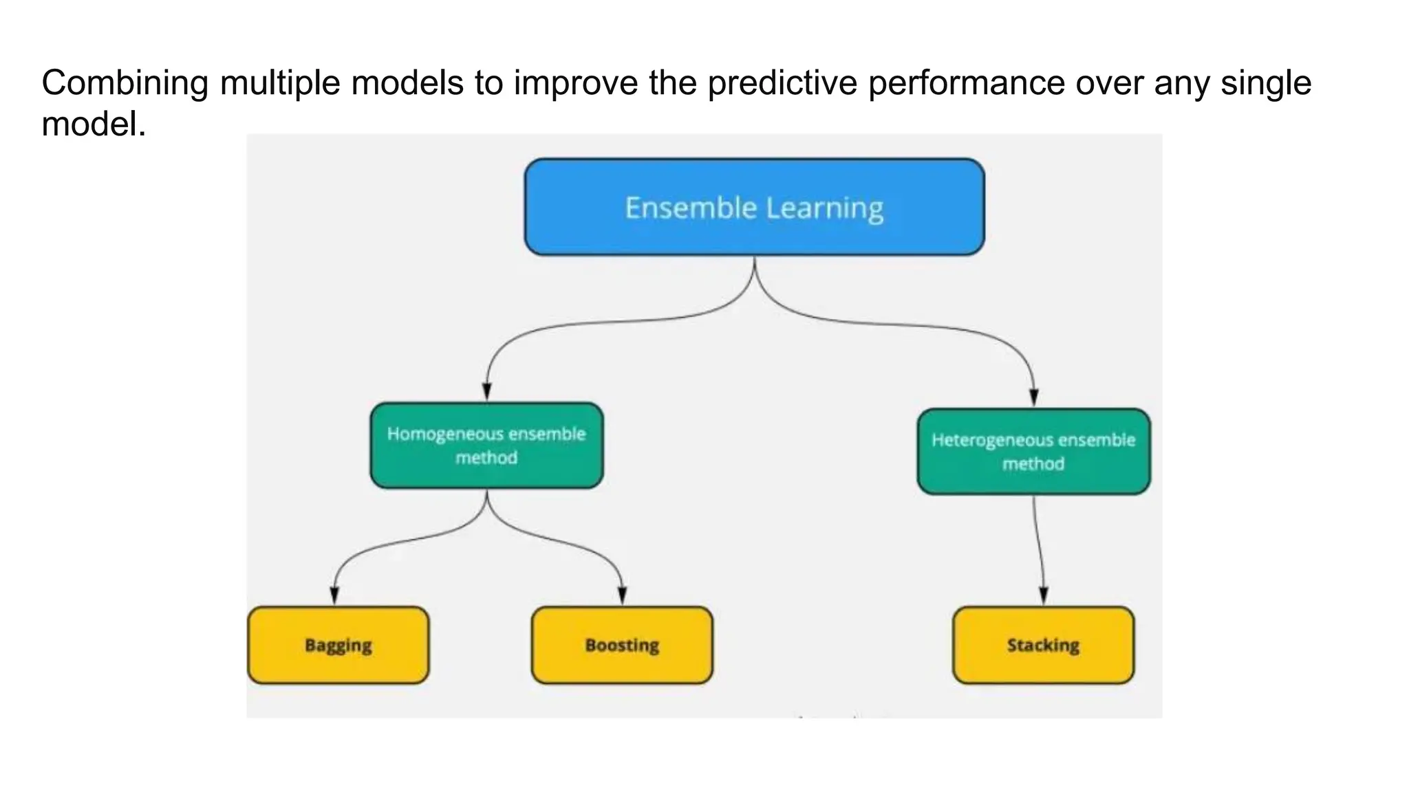
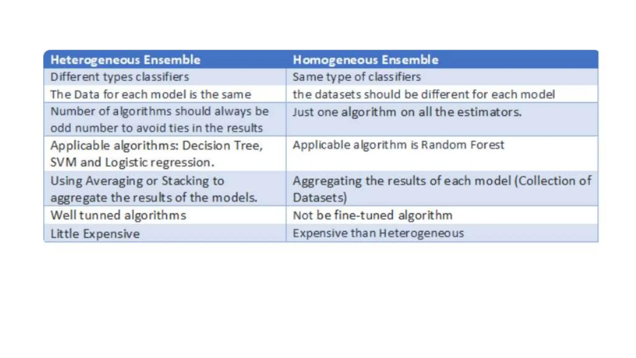
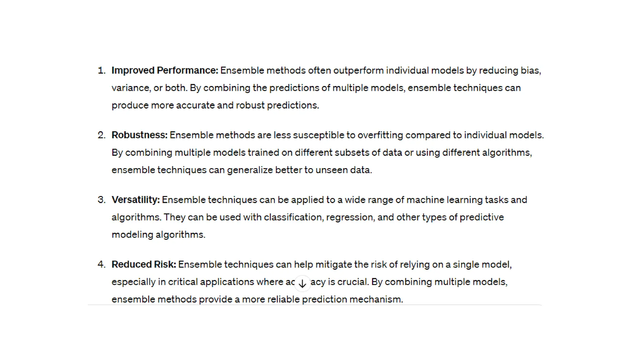
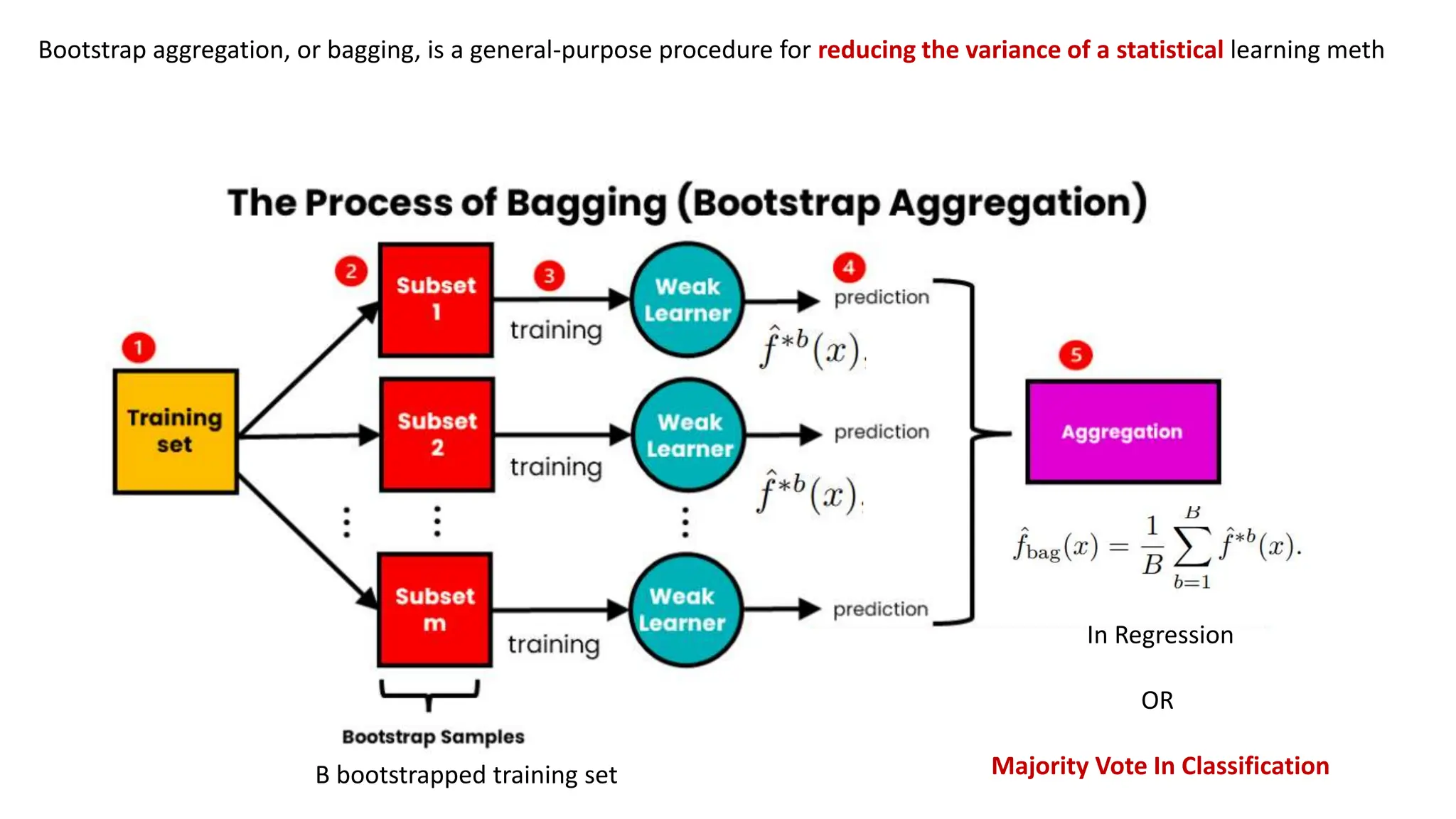
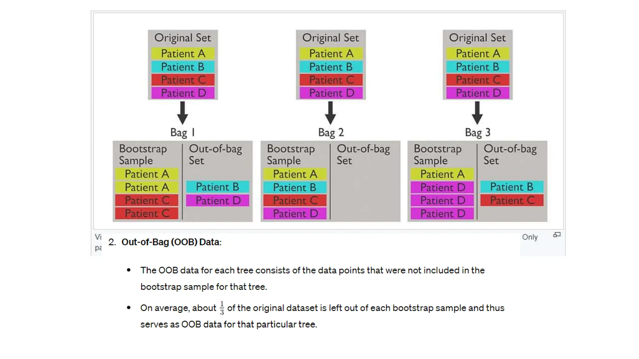
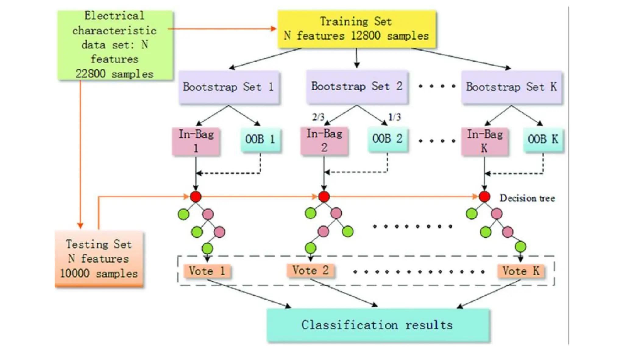
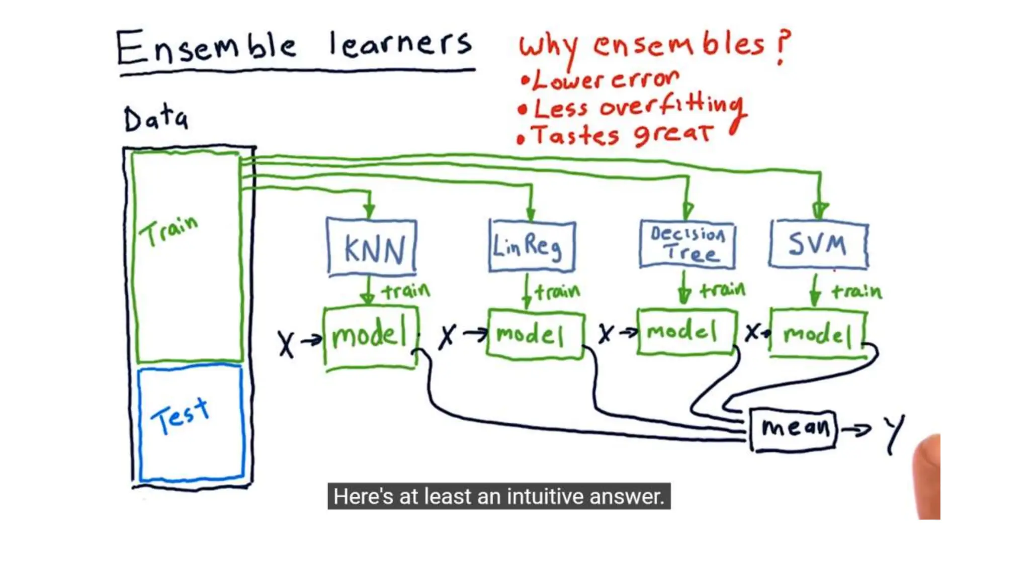

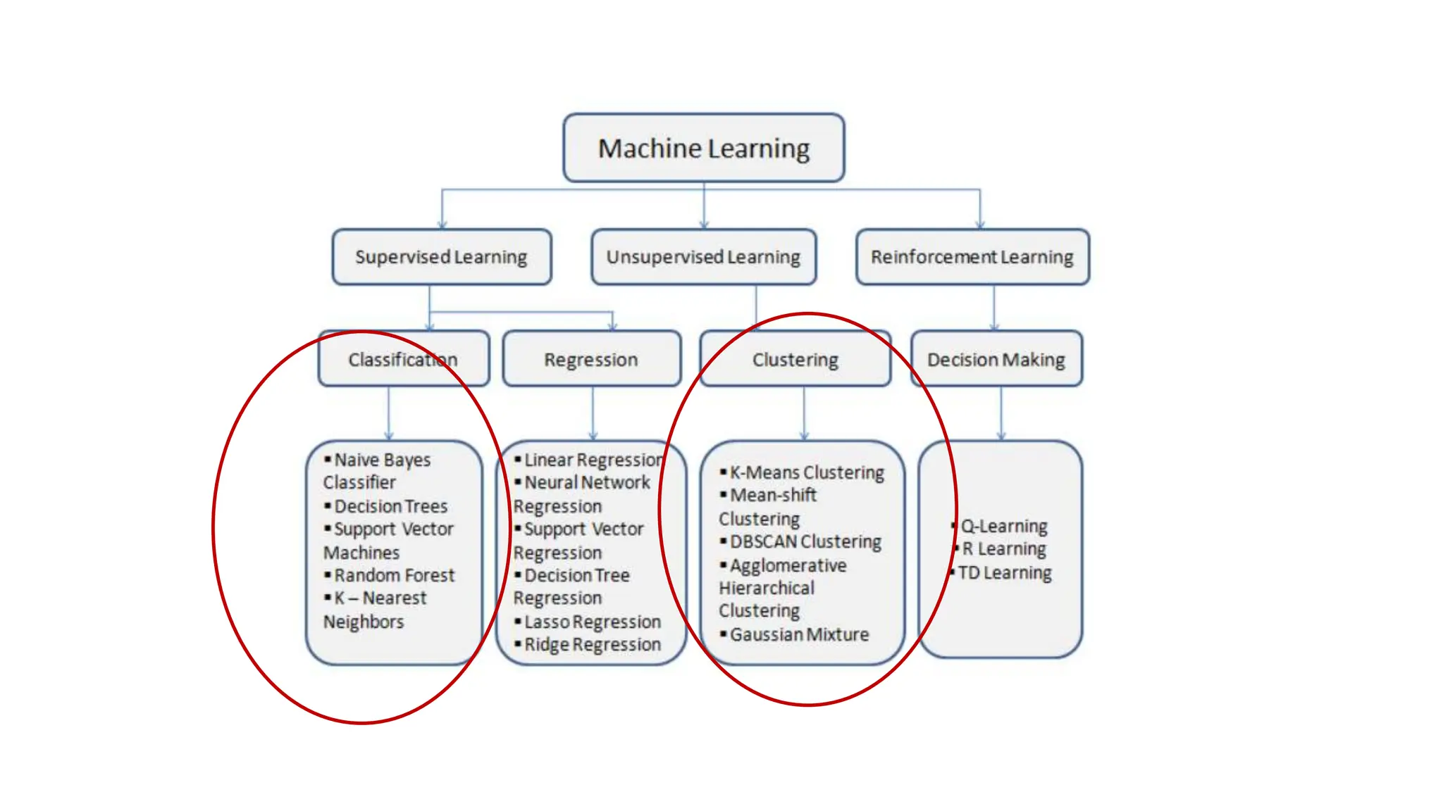
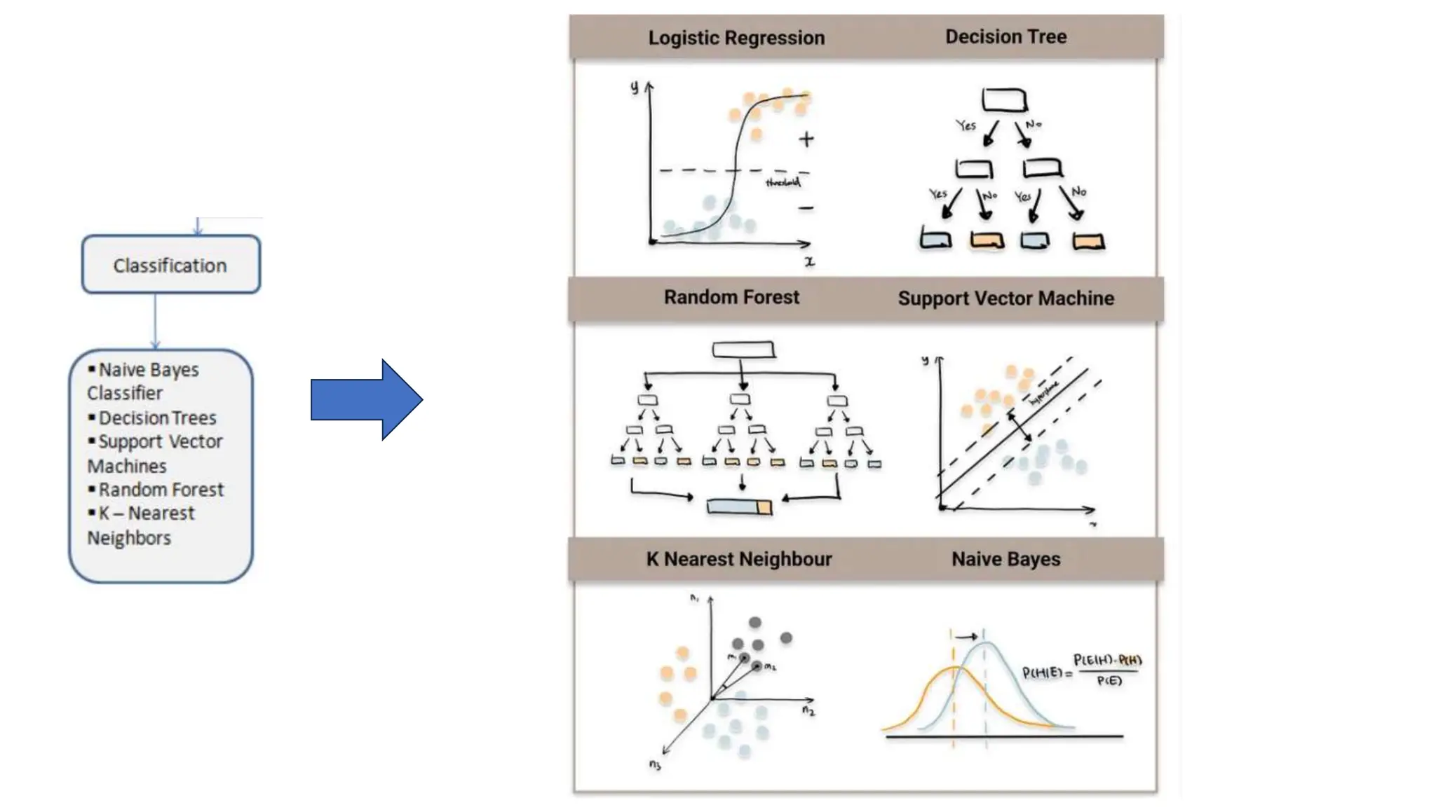
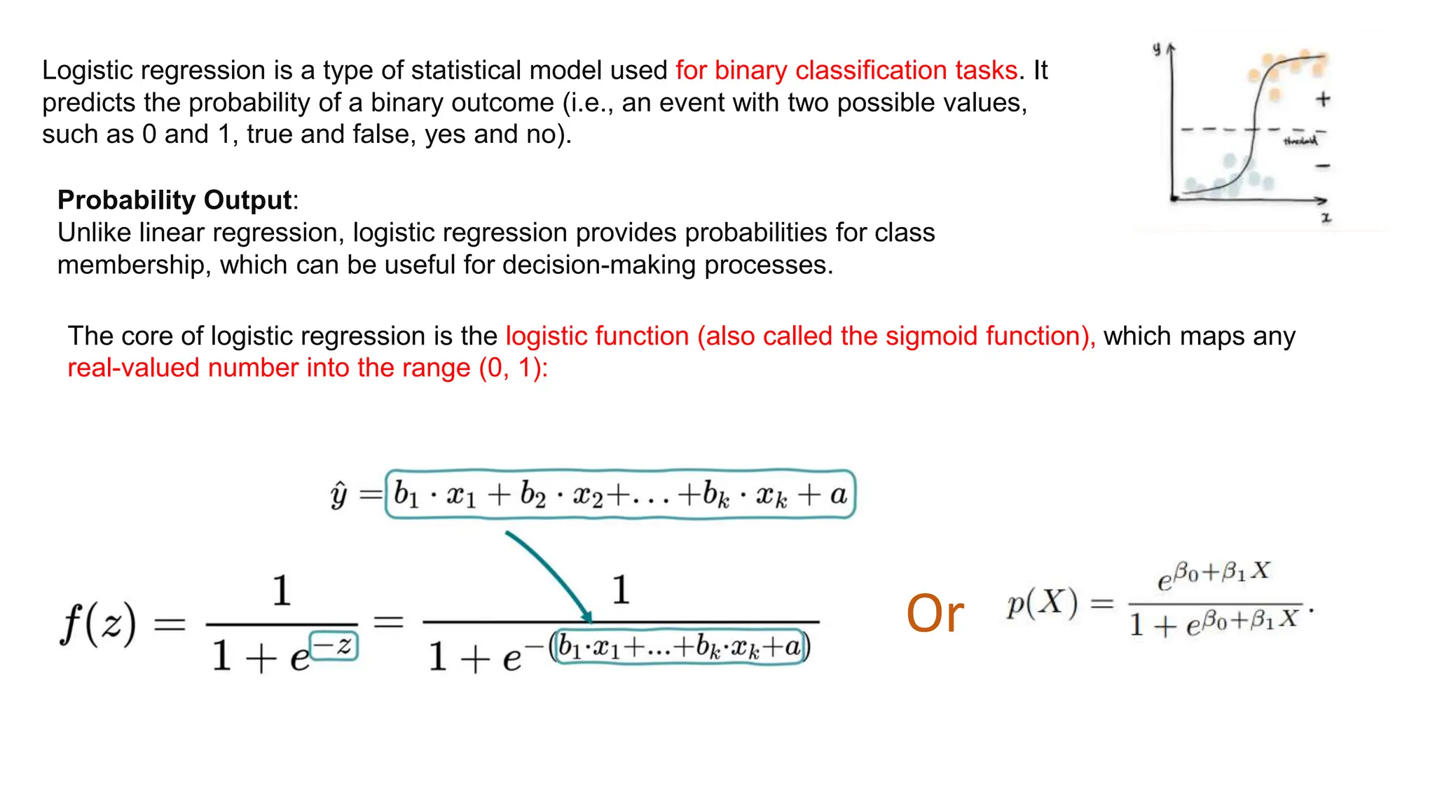
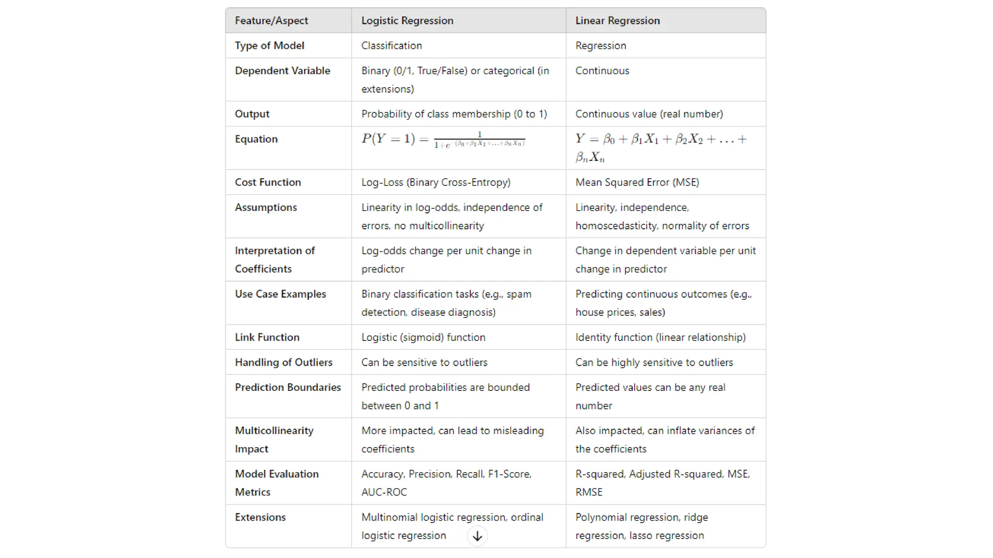
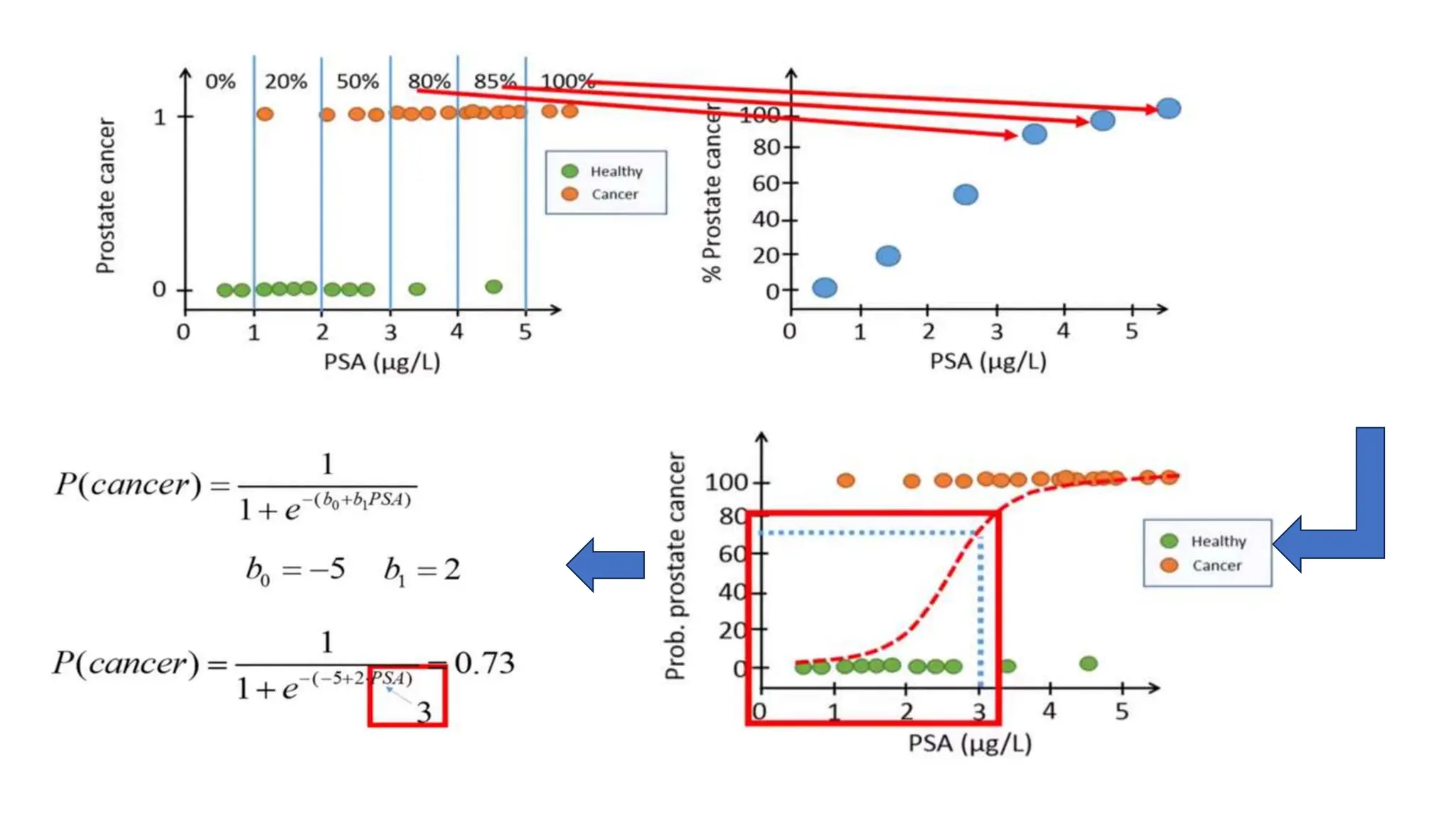
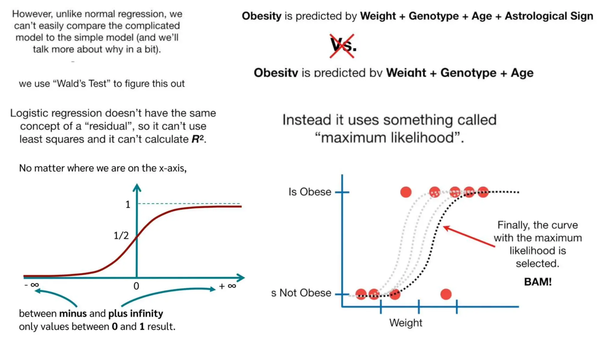

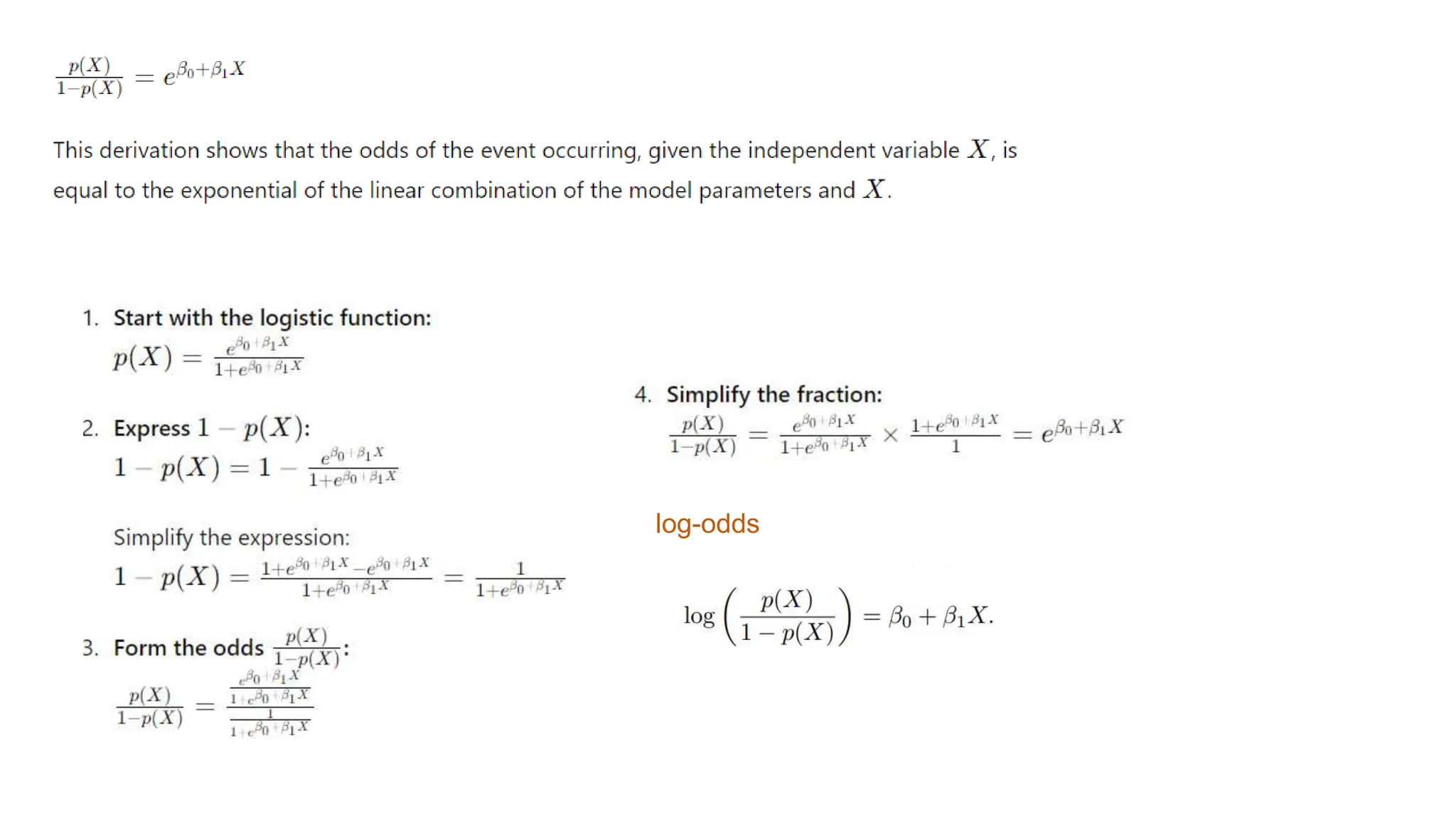
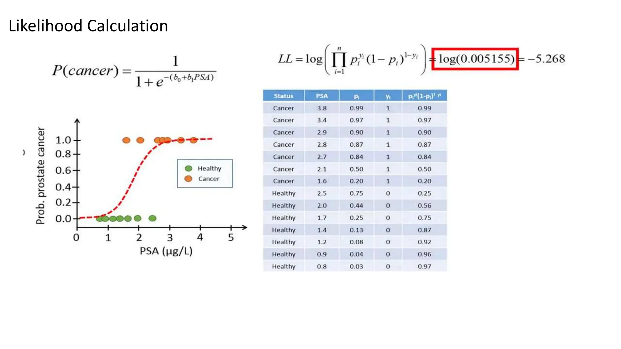
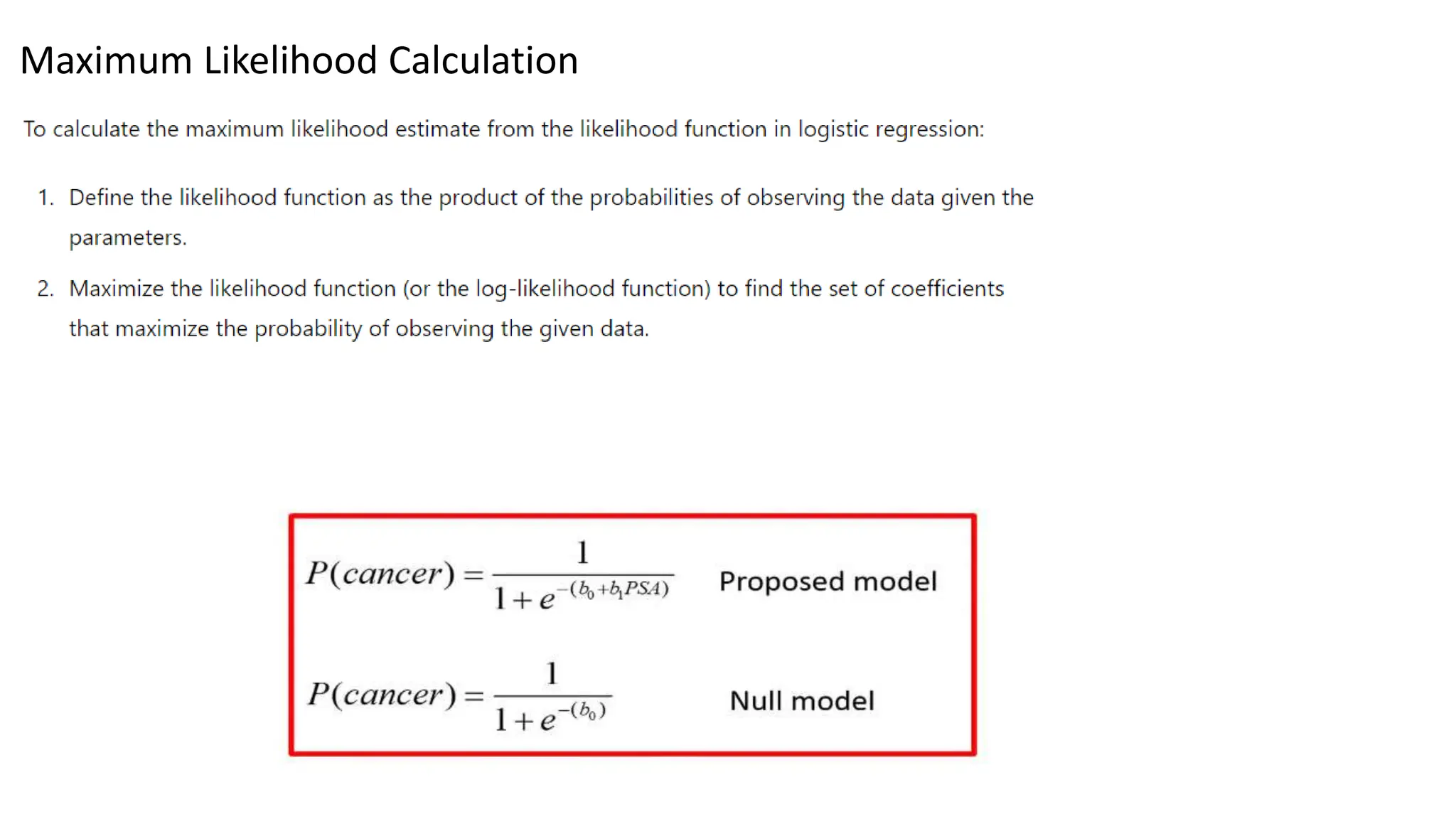
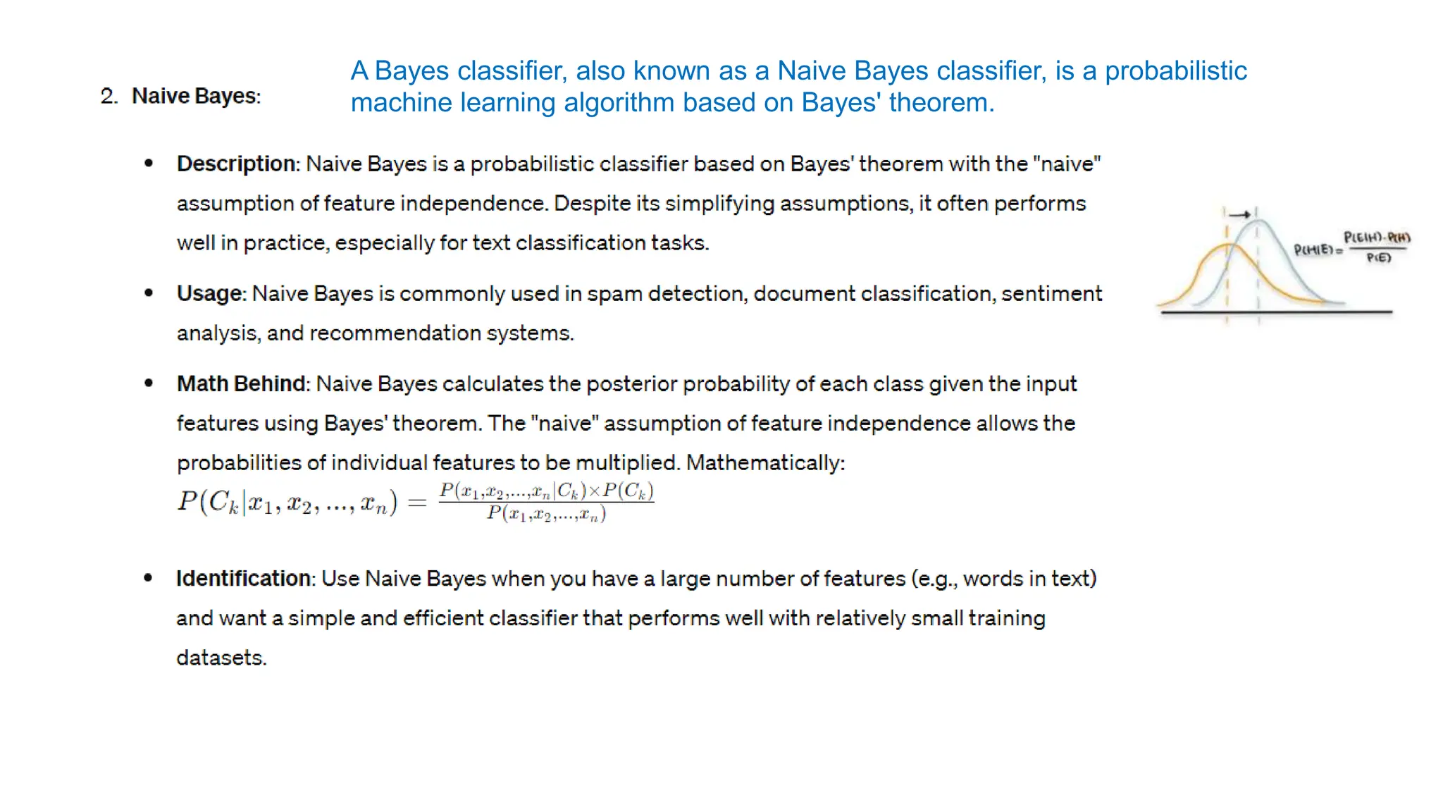


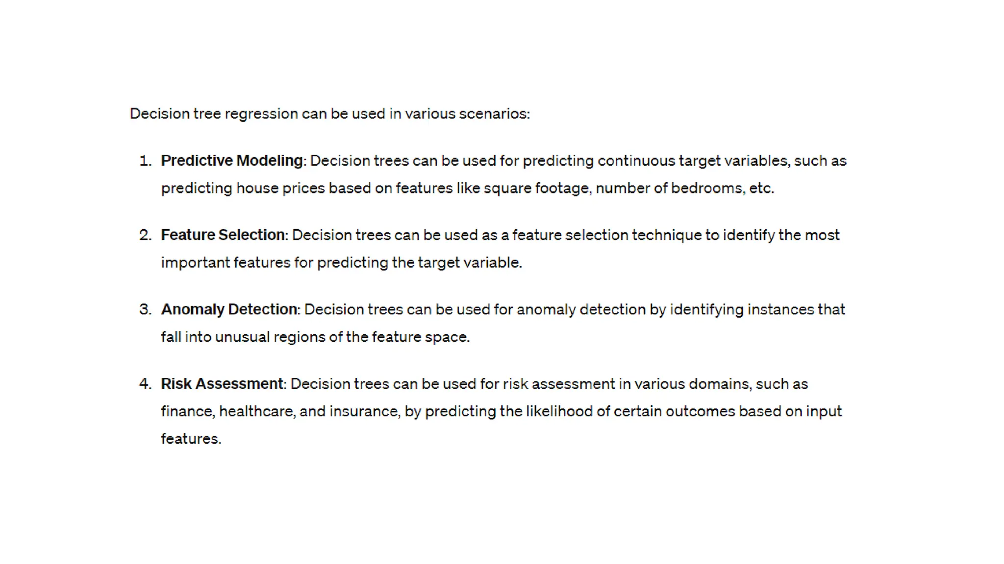
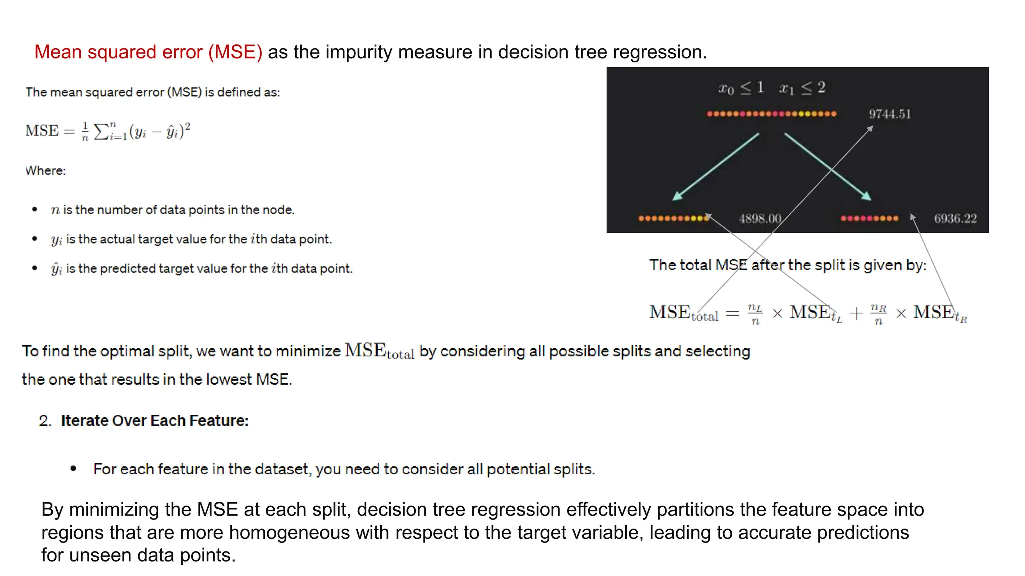


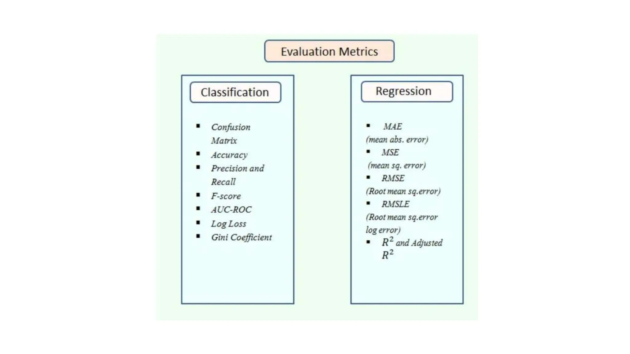
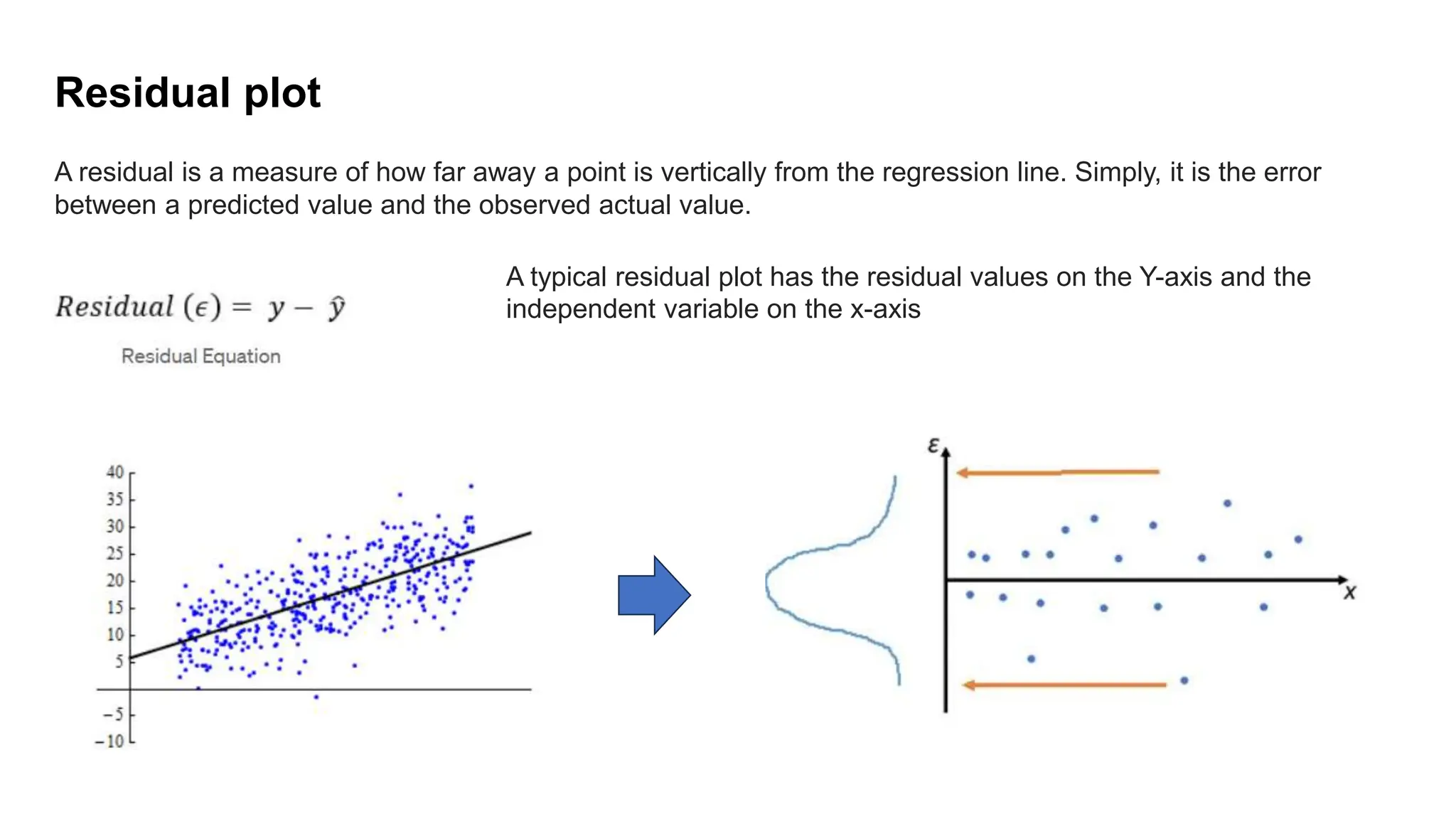
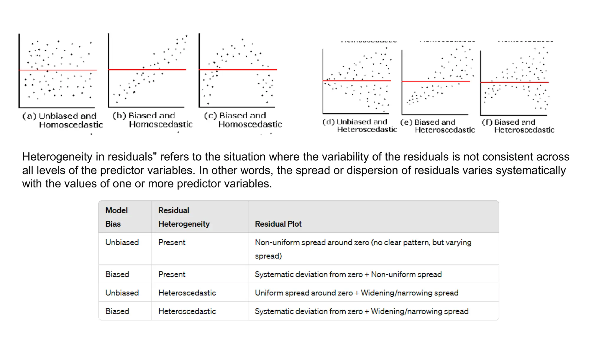
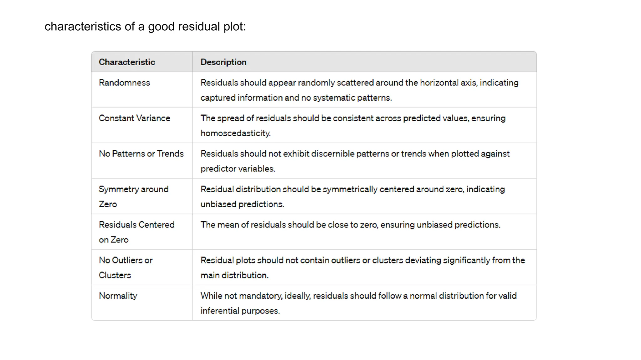
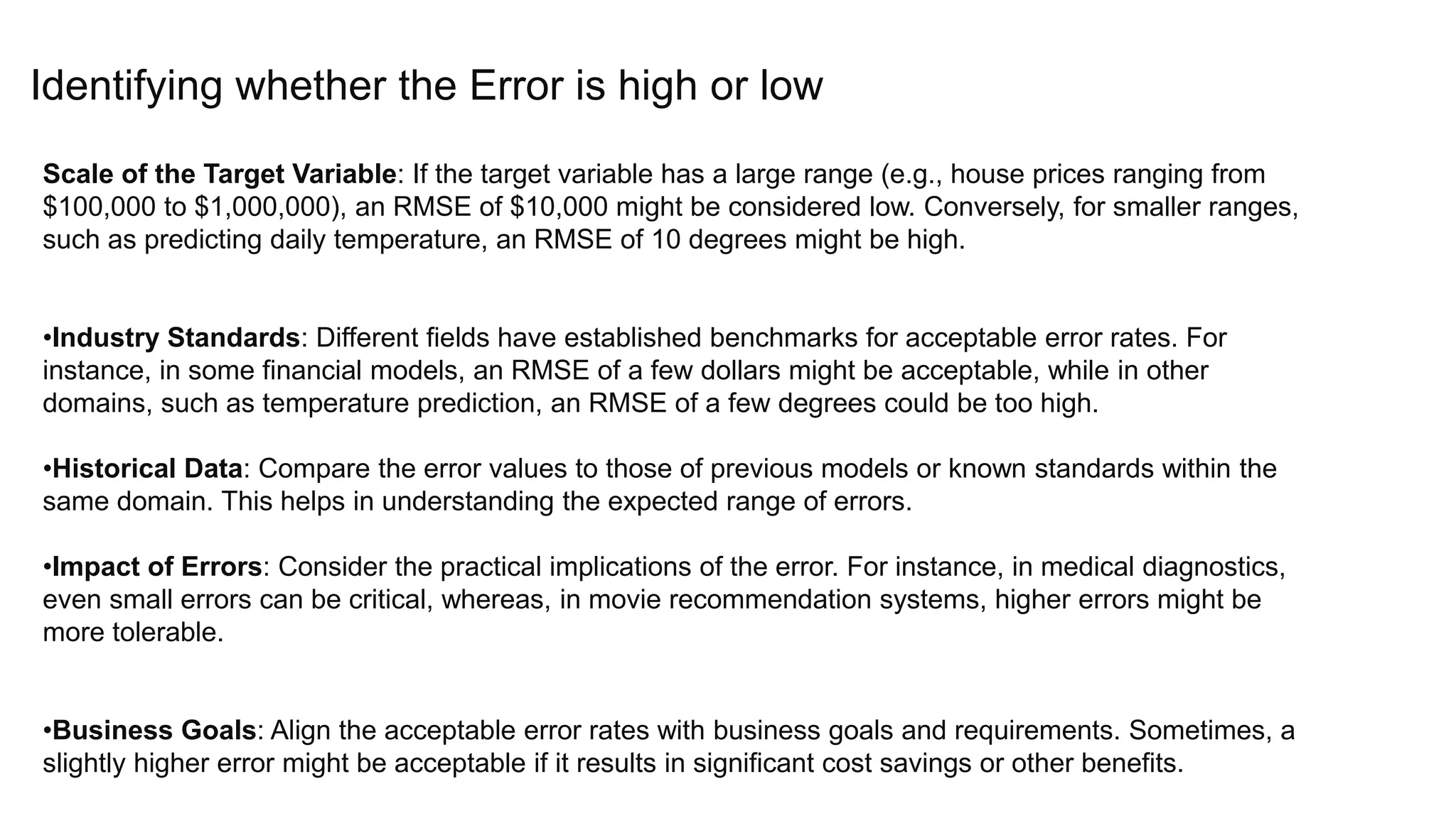
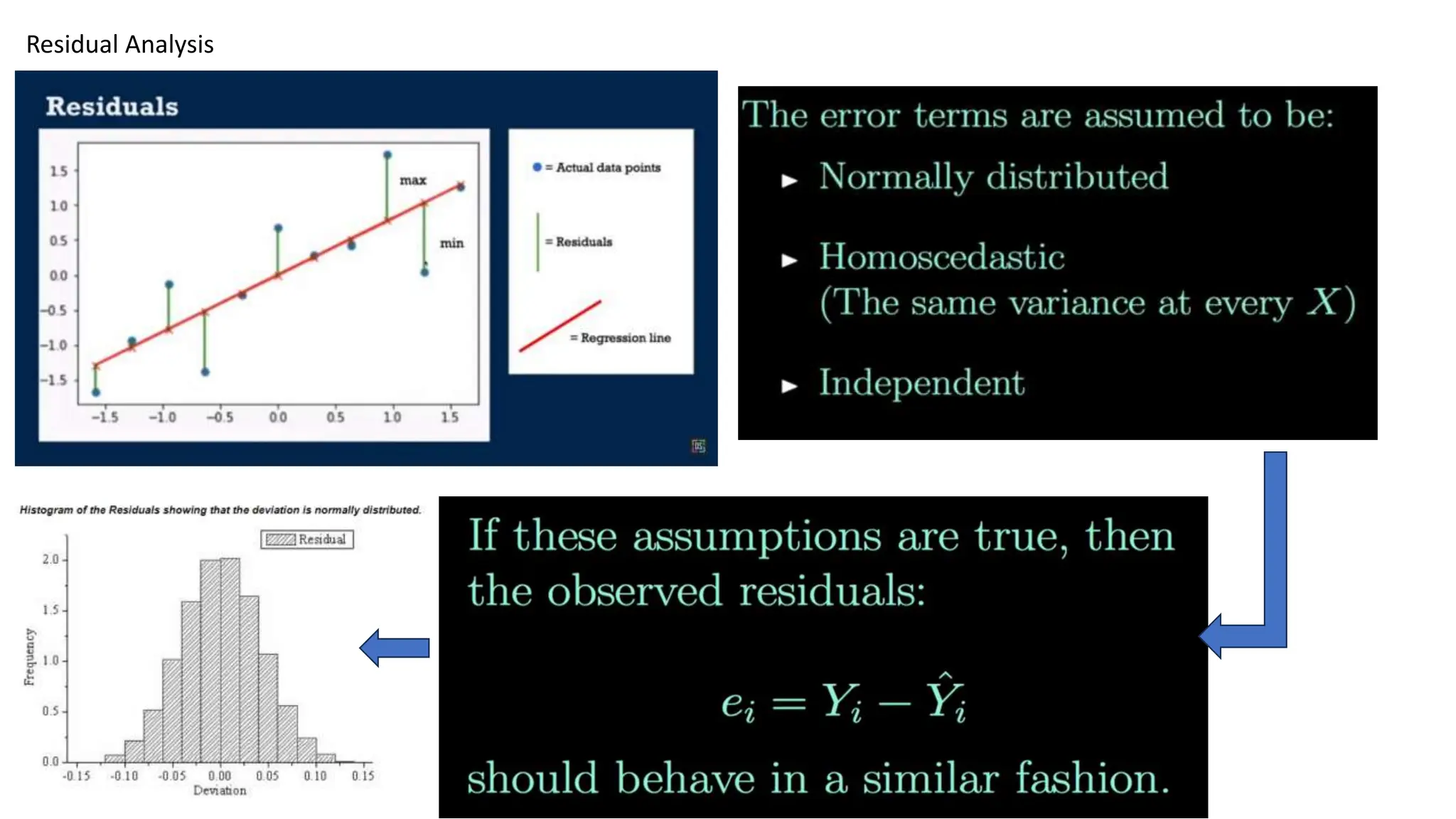
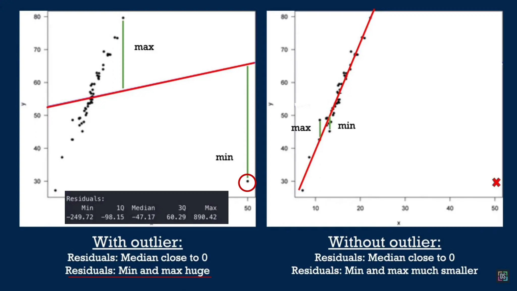
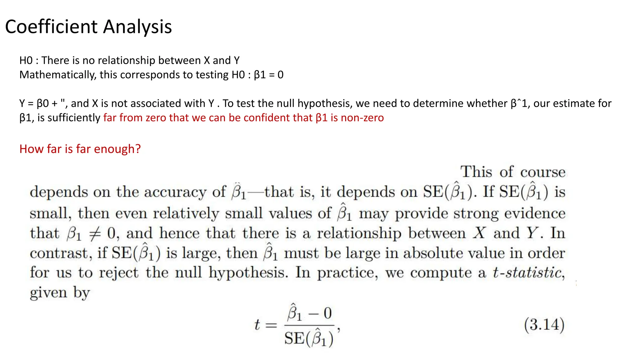
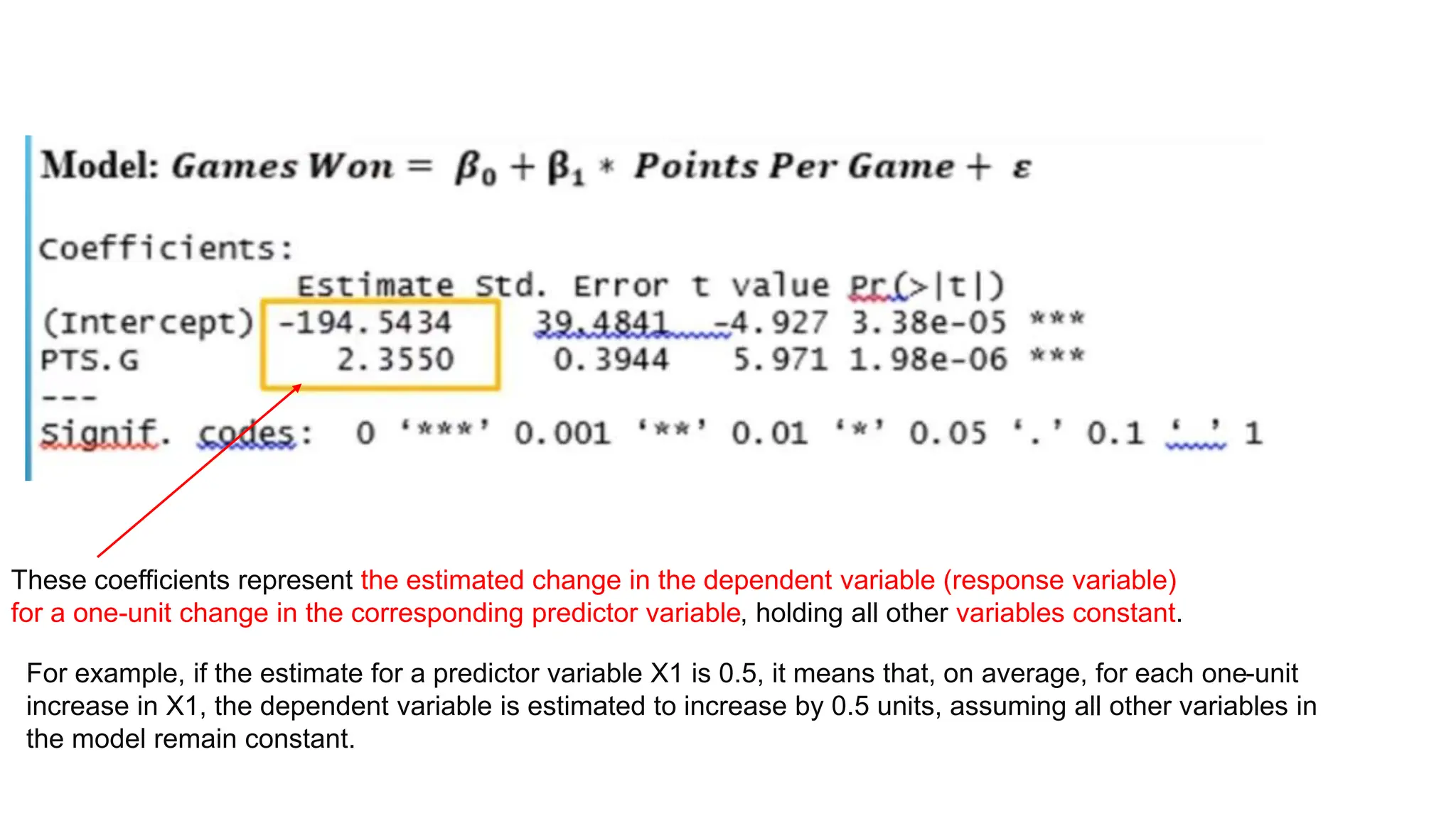


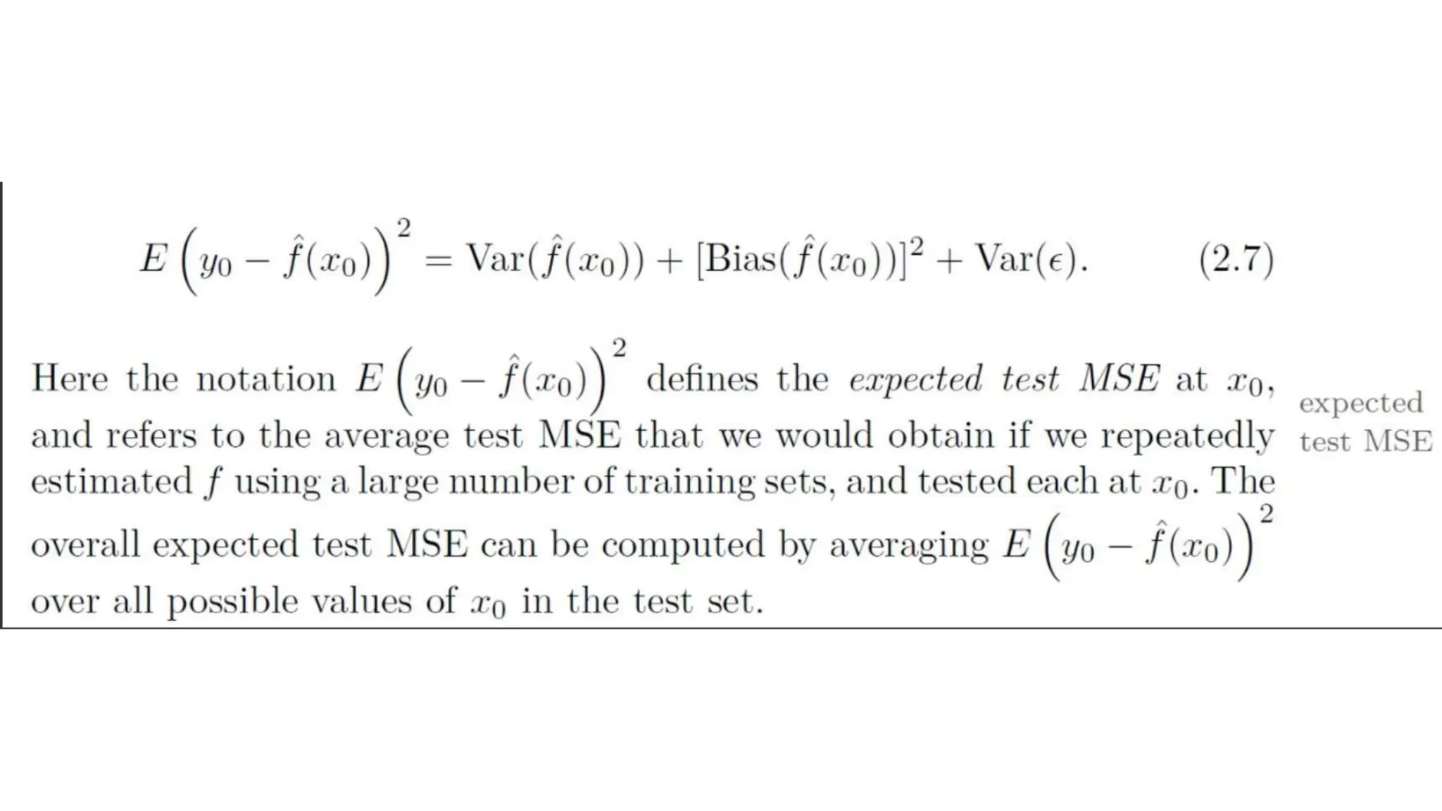
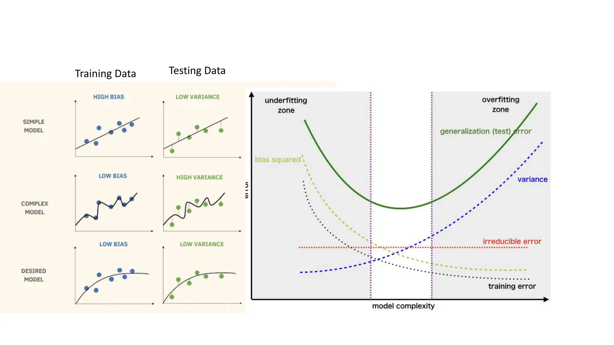
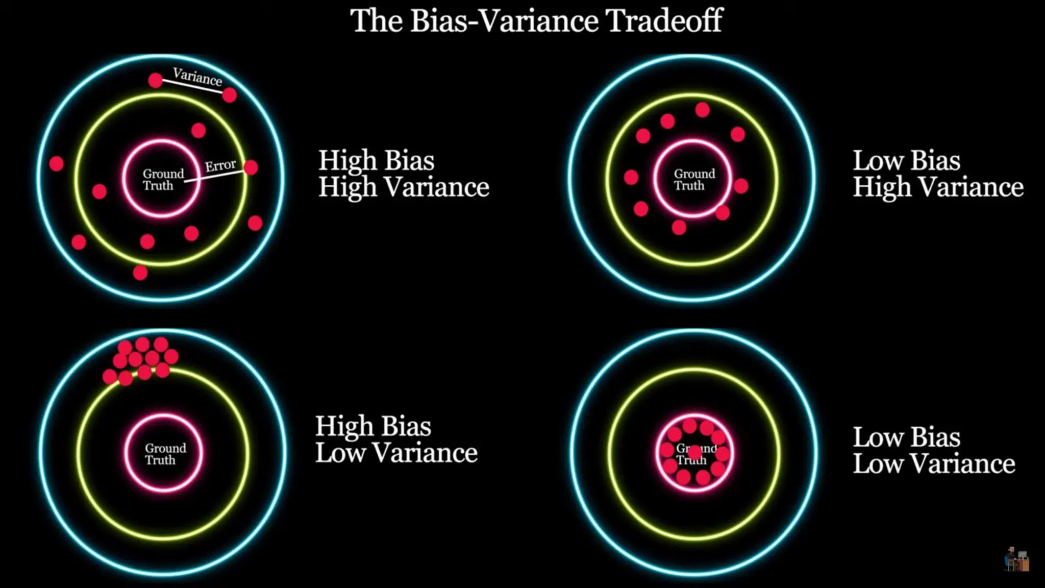


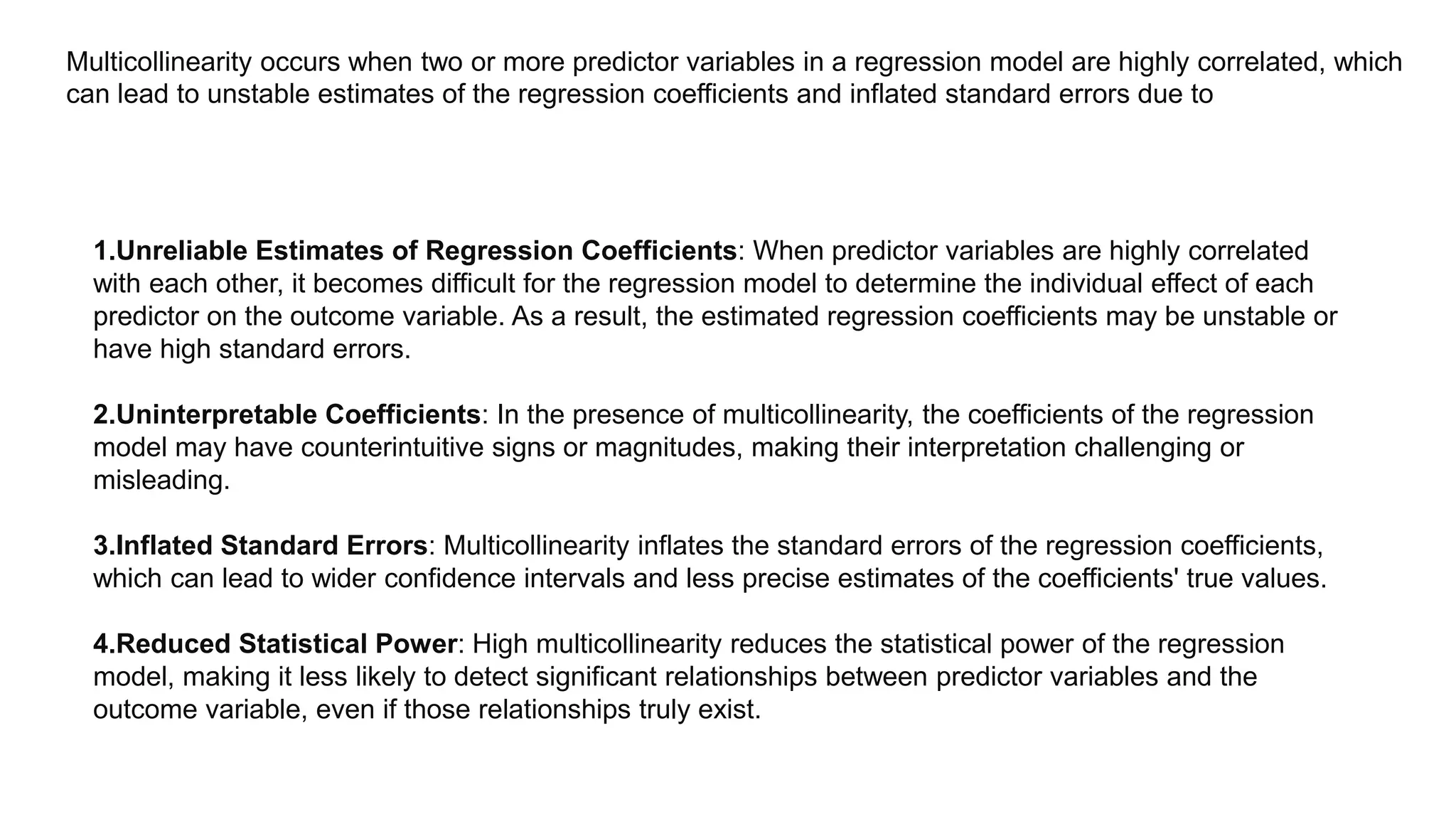
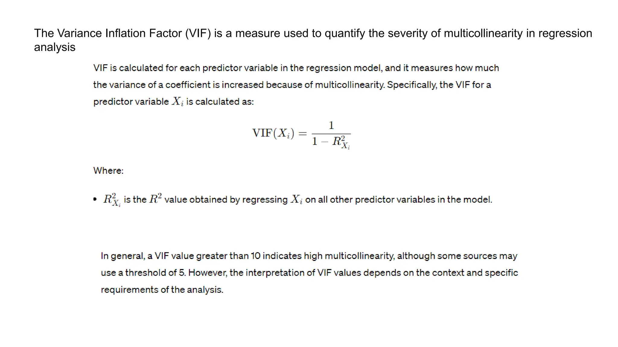

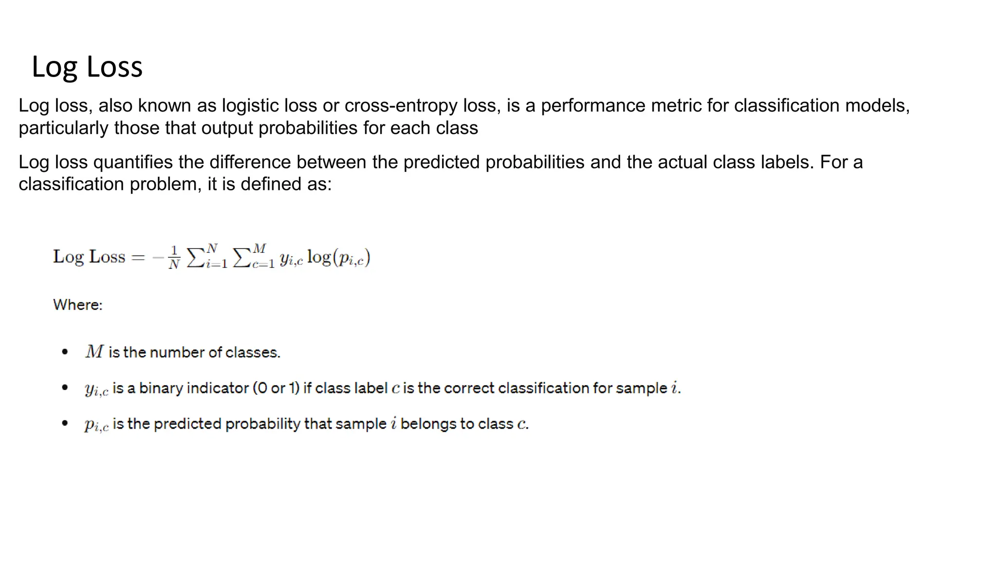
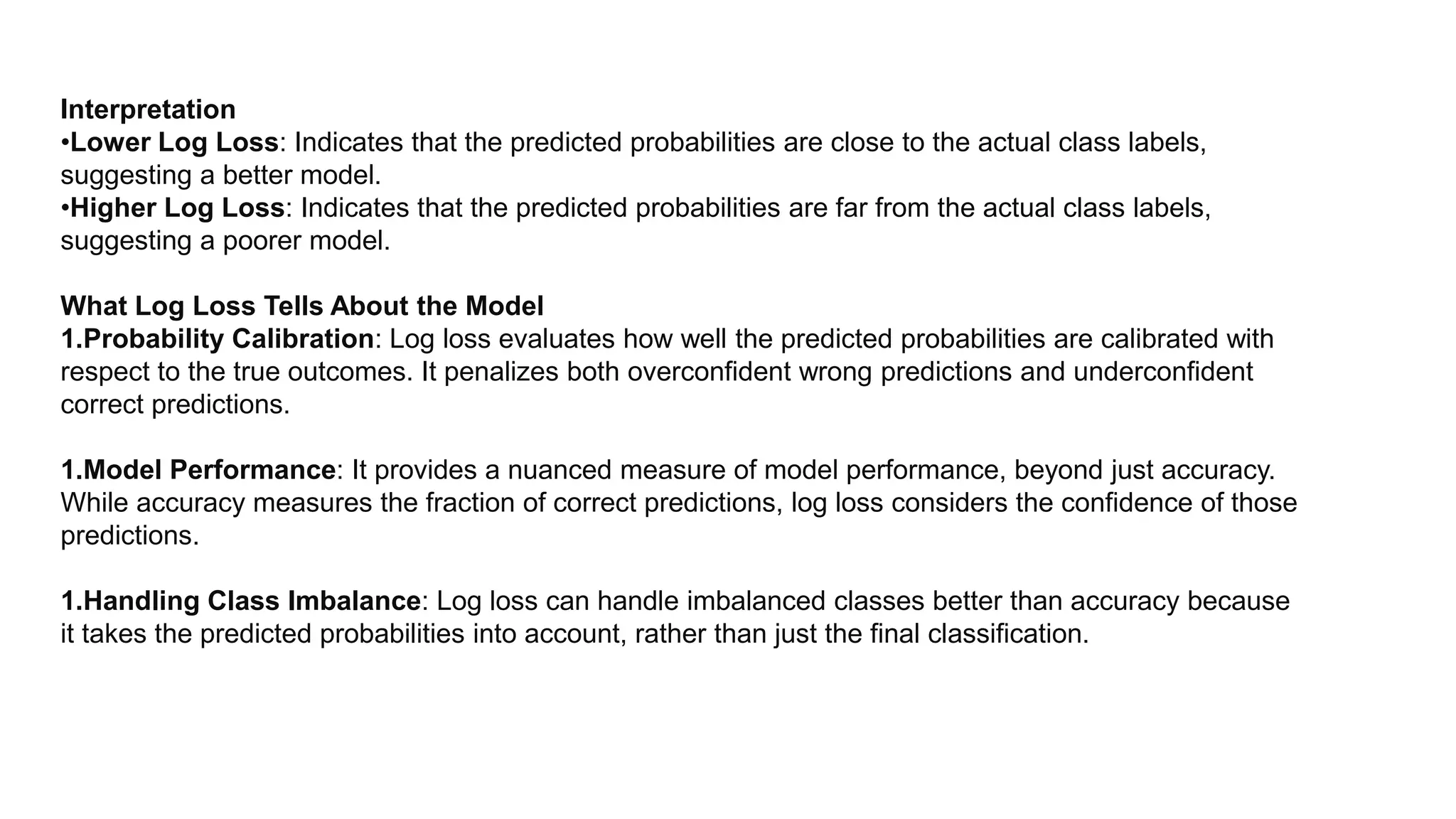
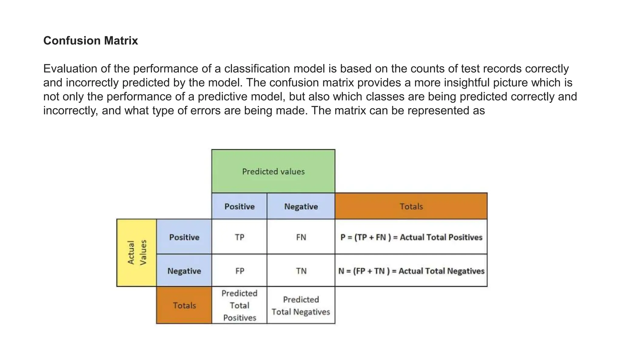
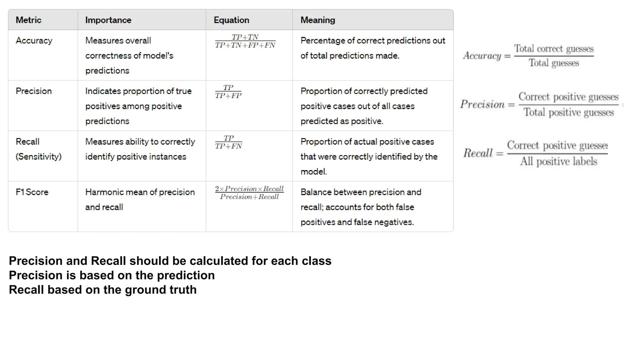
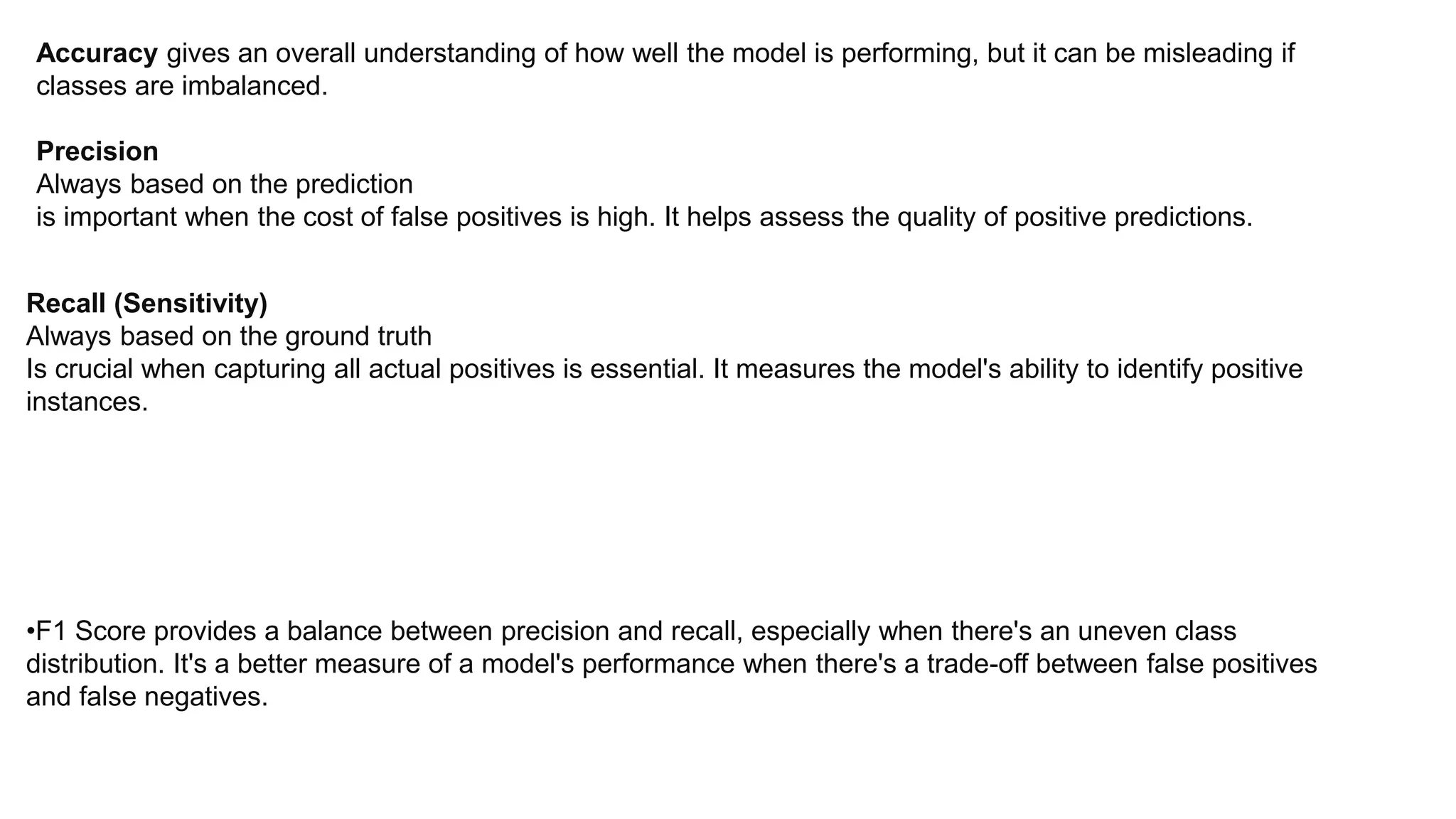
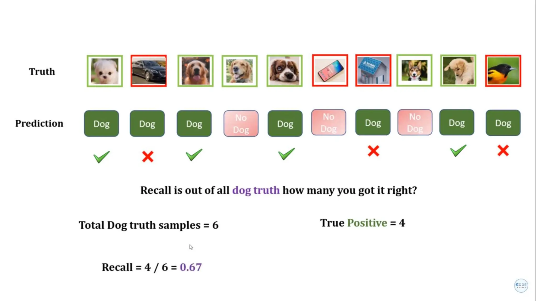
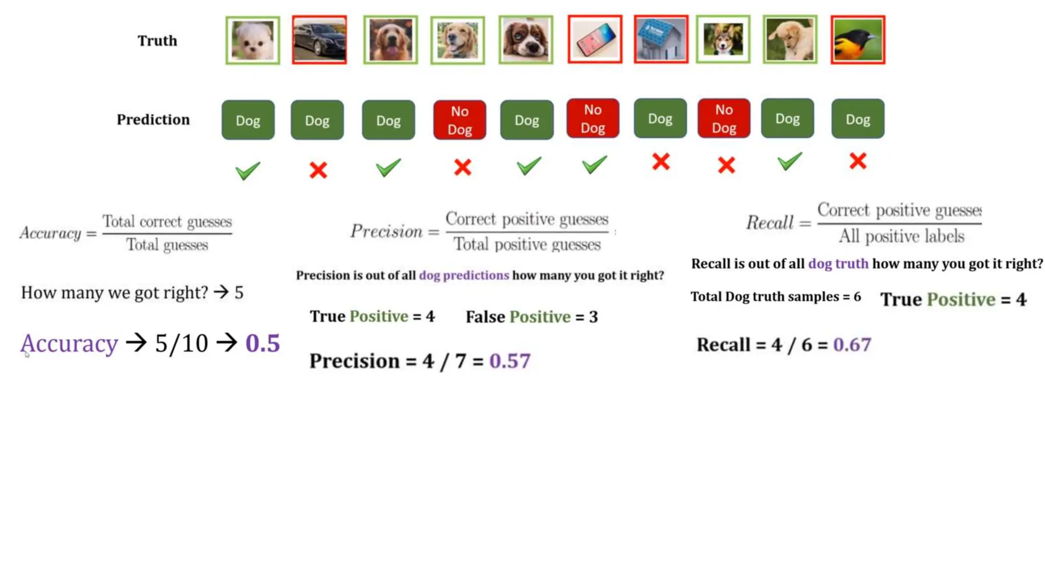
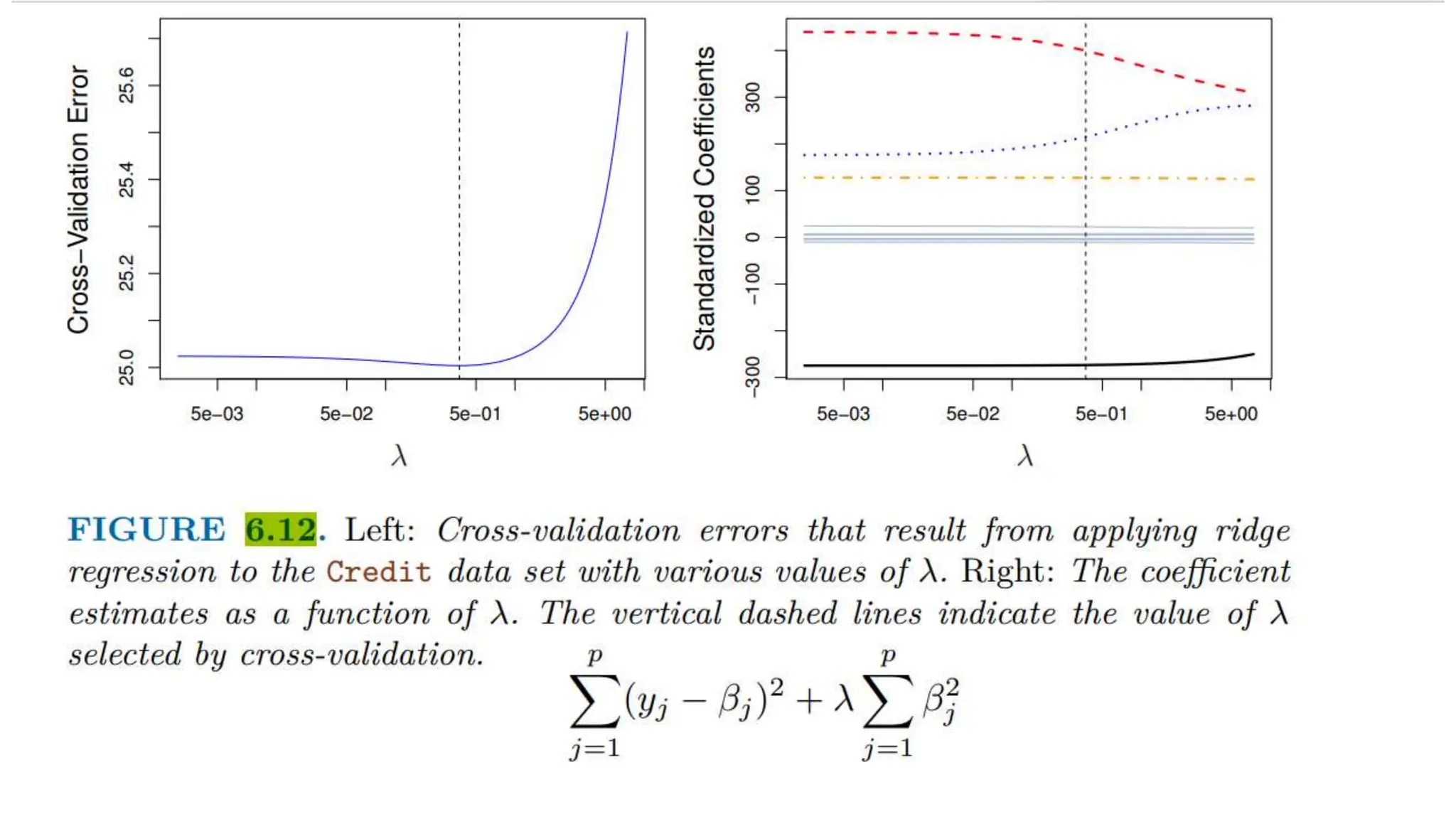
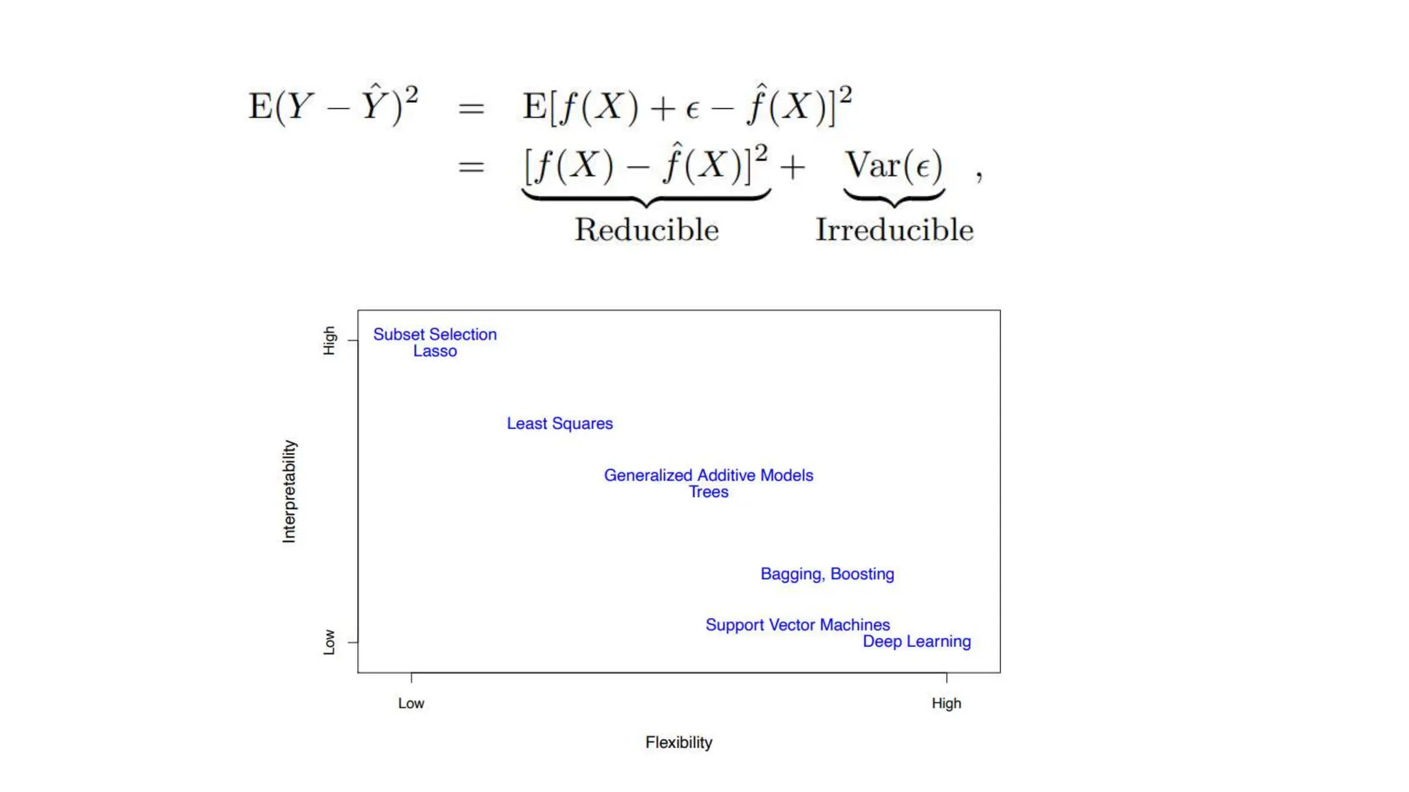
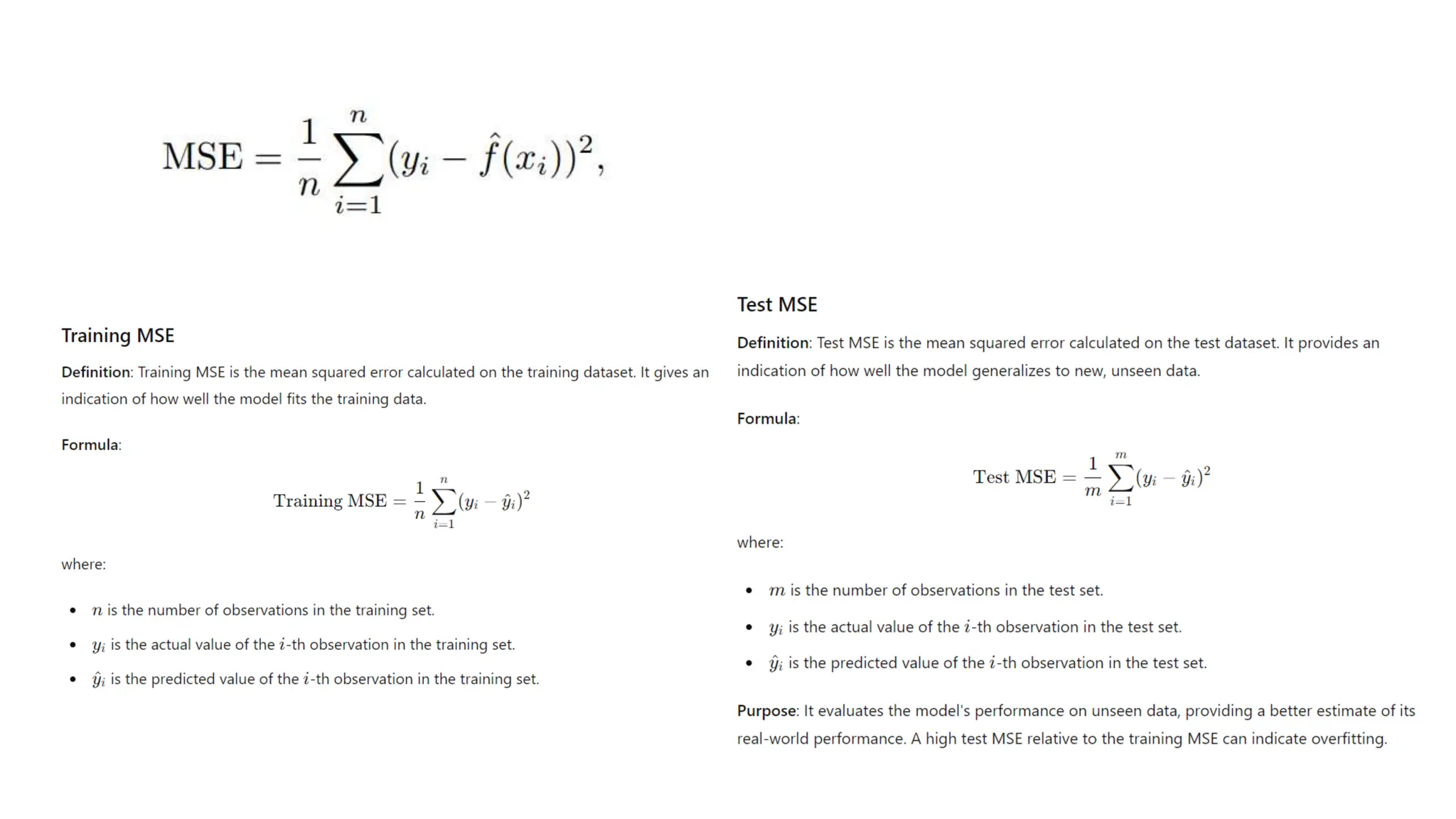
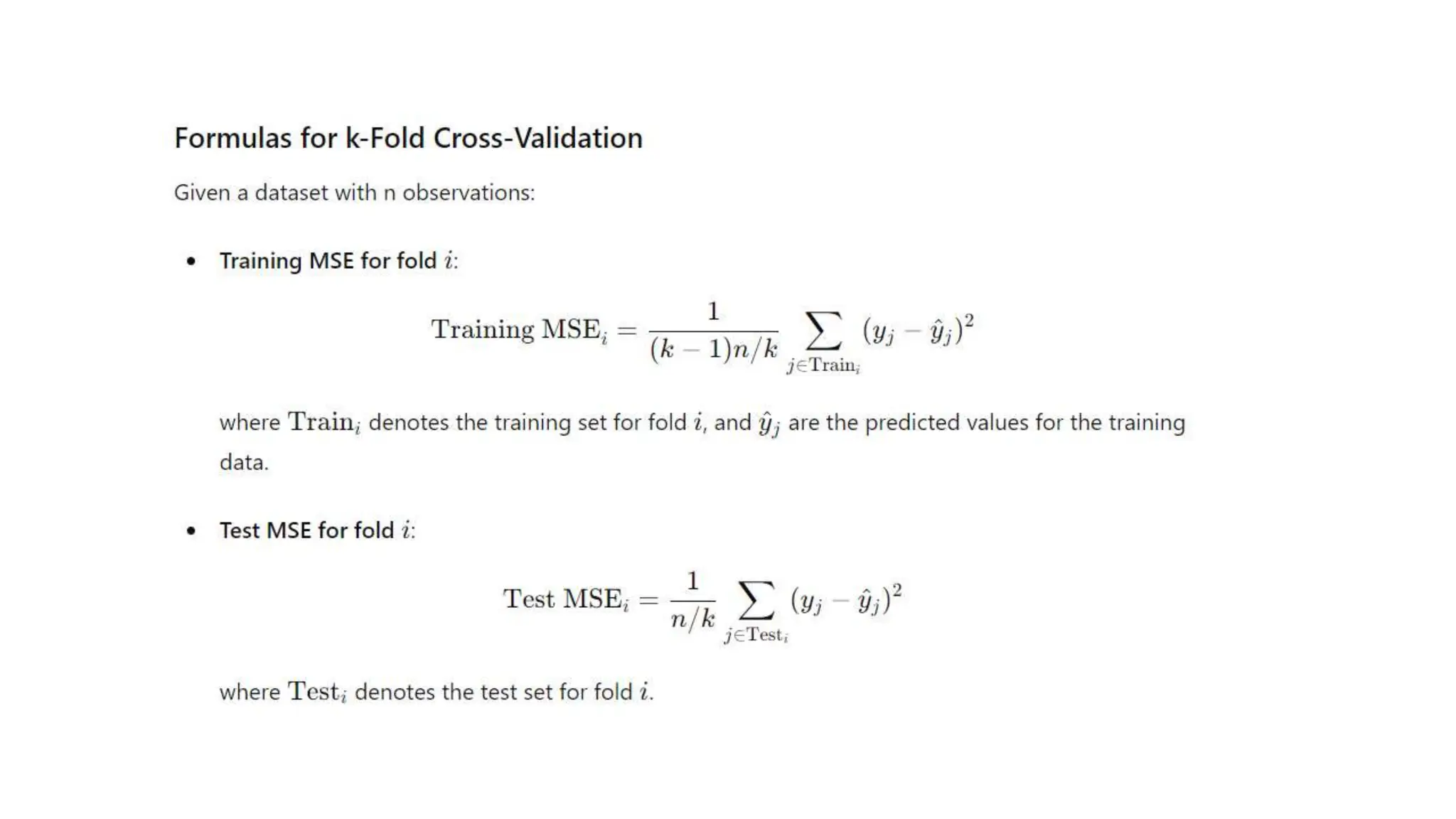

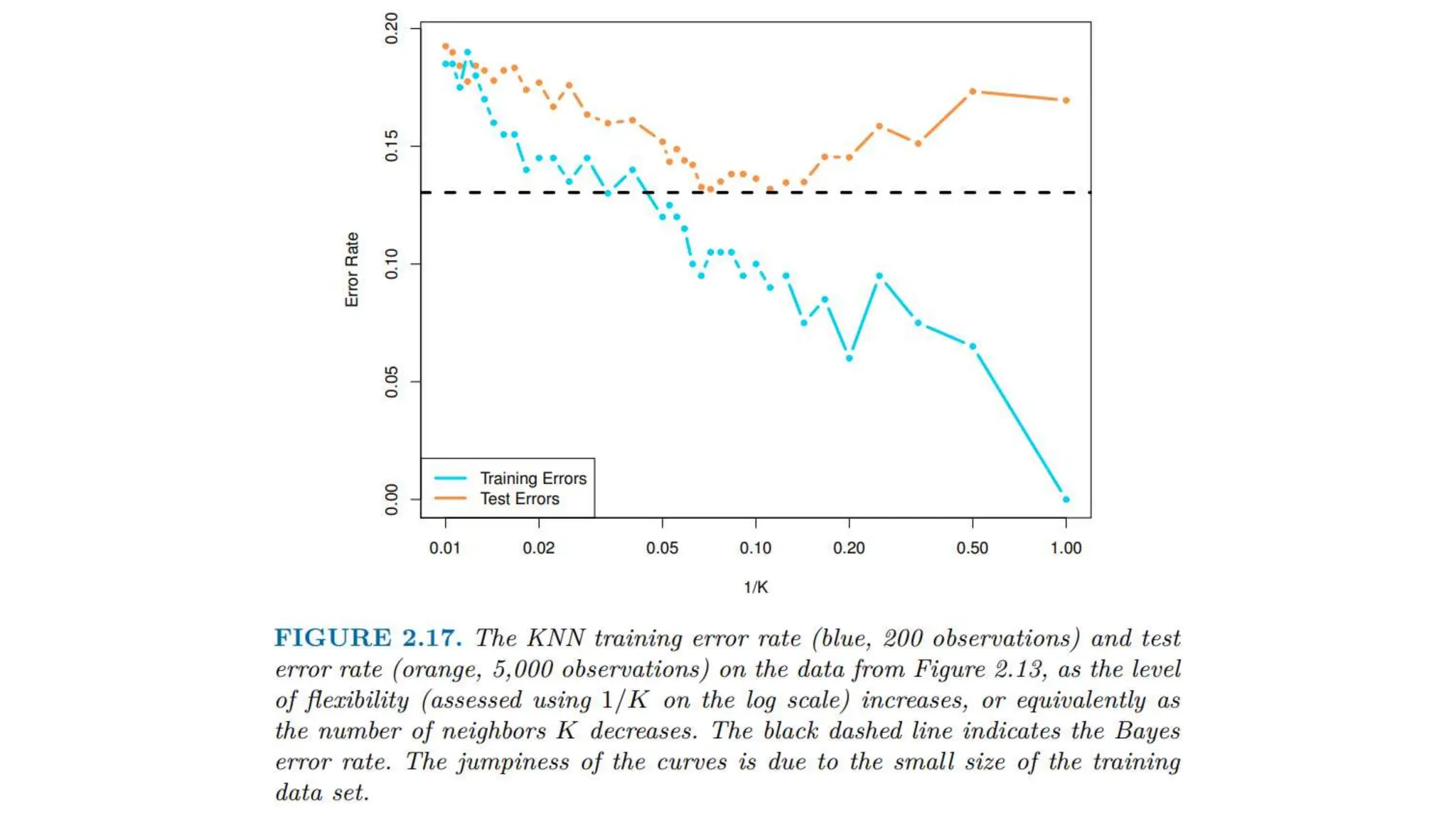
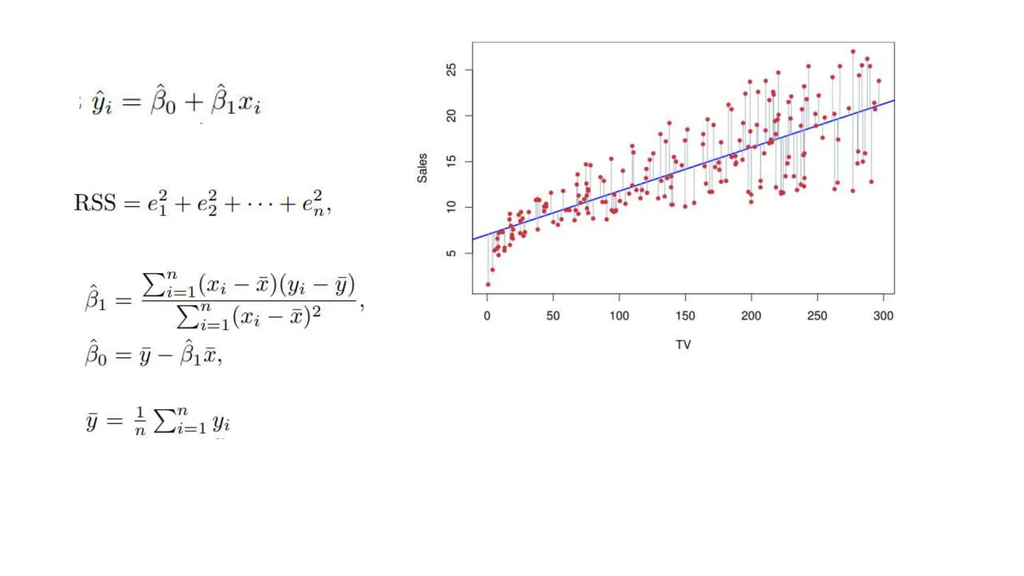
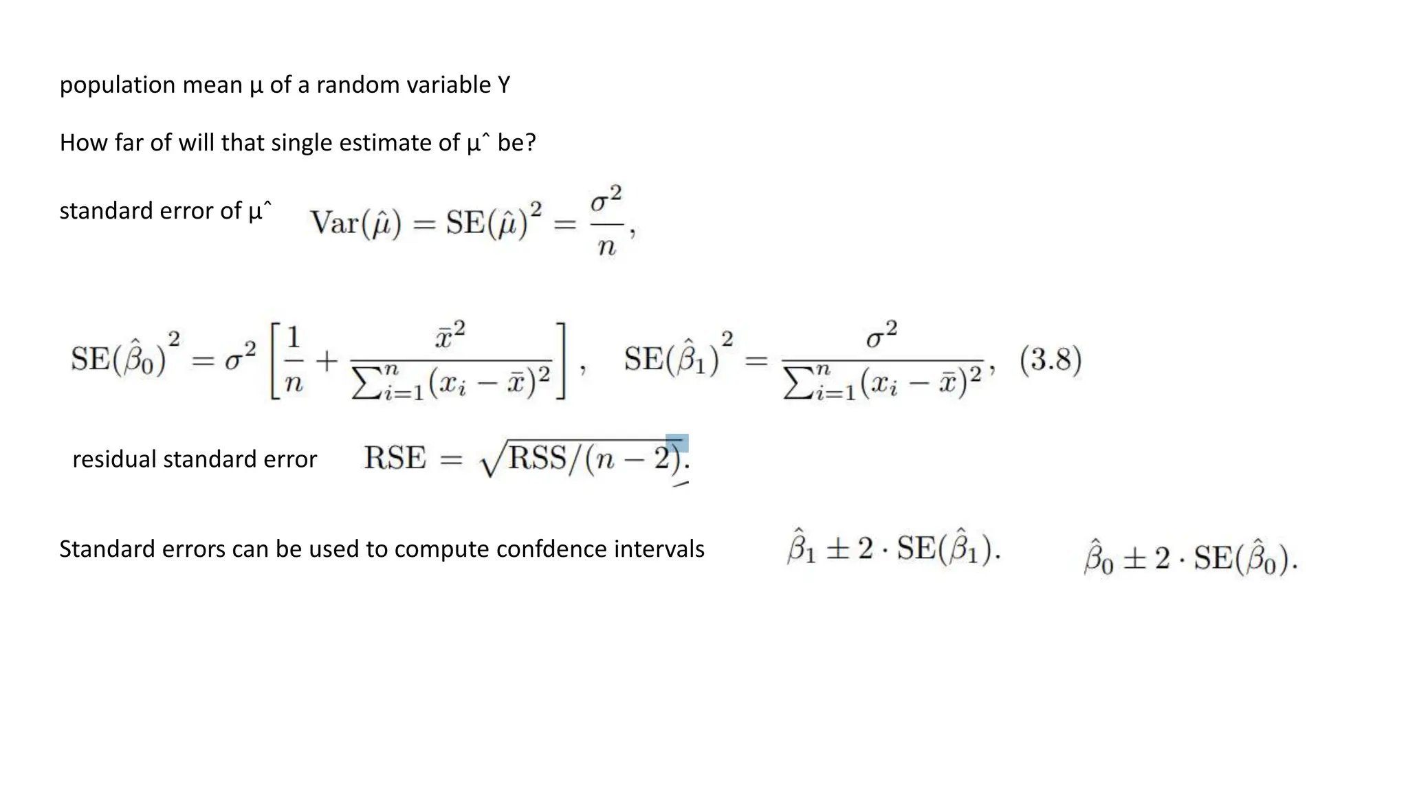
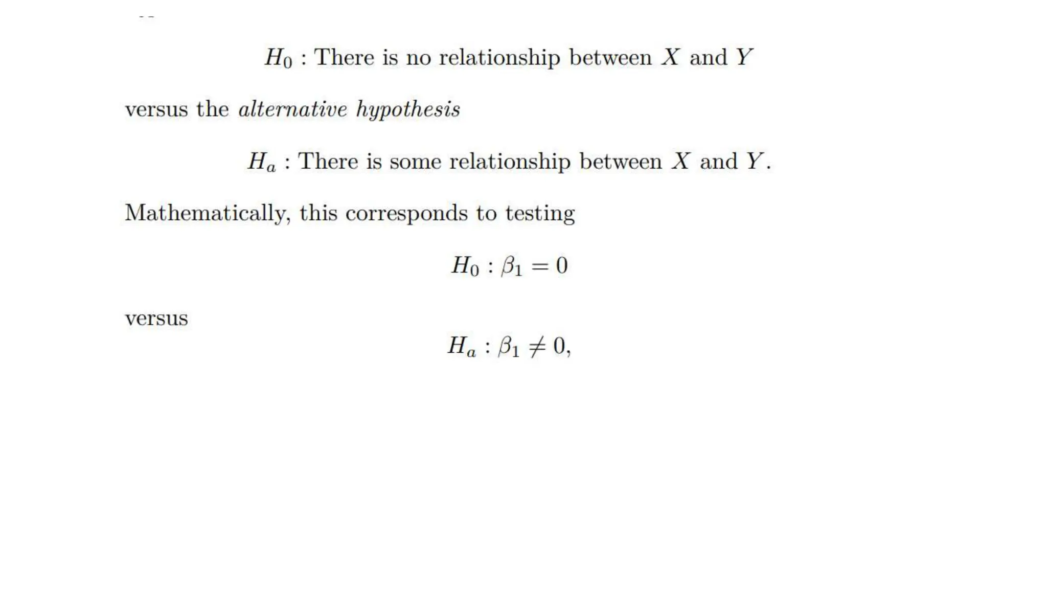


The document provides an overview of data science fundamentals, including data types, statistical measures, relationships among data, and machine learning concepts. It discusses the importance of exploratory data analysis (EDA), feature engineering, and feature selection techniques to improve model performance. Additionally, it distinguishes between PCA and traditional feature selection methods while highlighting their applications in machine learning.


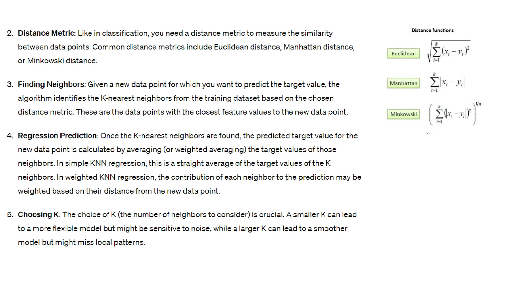
![[DSC Europe 25] Vid Stimac - Policy Parsimony: Between Oversimplifying and Ov...](https://cdn.slidesharecdn.com/ss_thumbnails/eqlepagzqp2rhg3gbluh-dsc-stimac-251120-251205090438-059e7f54-thumbnail.jpg?width=640&height=640&fit=bounds)
![[DSC Europe 25] Bogdan Daniel Maruneac - AI - It starts with you.pptx](https://cdn.slidesharecdn.com/ss_thumbnails/odov3snhrcqs9hx5ny2n-4-251205085715-f1daacfe-thumbnail.jpg?width=640&height=640&fit=bounds)


![[DSC Europe 25] Boris Perkovic - Lost in performance.pptx](https://cdn.slidesharecdn.com/ss_thumbnails/uq5hrp7vsuahqkxzifux-1-251204082258-fd2ee09d-thumbnail.jpg?width=640&height=640&fit=bounds)