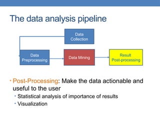
Data mining involves analyzing large data sets to extract useful patterns and summarize data in comprehensible ways, facilitating knowledge discovery for commercial or scientific purposes. It encompasses various models, including predictive, explanatory, and summarization models, using diverse data types such as numeric, categorical, and relational data. The data mining pipeline consists of steps like data collection, preprocessing, mining, and post-processing, emphasizing the importance of data quality and structured storage.

1. DATA MINING
LECTURE 2
What is data?
The data mining pipeline

2. What is Data Mining?
• Data mining is the use of efficient techniques for the analysis of very
large collections of data and the extraction of useful and possibly
unexpected patterns in data.
• “Data mining is the analysis of (often large) observational data sets to
find unsuspected relationships and to summarize the data in novel
ways that are both understandable and useful to the data analyst”
(Hand, Mannila, Smyth)
• “Data mining is the discovery of models for data” (Rajaraman, Ullman)
• We can have the following types of models
• Models that explain the data (e.g., a single function)
• Models that predict the future data instances.
• Models that summarize the data
• Models the extract the most prominent features of the data.

3. Why do we need data mining?
• Really huge amounts of complex data generated from multiple sources
and interconnected in different ways
• Scientific data from different disciplines
• Weather, astronomy, physics, biological microarrays, genomics
• Huge text collections
• The Web, scientific articles, news, tweets, facebook postings.
• Transaction data
• Retail store records, credit card records
• Behavioral data
• Mobile phone data, query logs, browsing behavior, ad clicks
• Networked data
• The Web, Social Networks, IM networks, email network, biological networks.
• All these types of data can be combined in many ways
• Facebook has a network, text, images, user behavior, ad transactions.
• We need to analyze this data to extract knowledge
• Knowledge can be used for commercial or scientific purposes.
• Our solutions should scale to the size of the data

4. What is Data?
• Collection of data objects and their
attributes
• An attribute is a property or
characteristic of an object
• Examples: name, date of birth, height,
occupation.
• Attribute is also known as variable,
field, characteristic, or feature
• For each object the attributes take
some values.
• The collection of attribute-value pairs
describes a specific object
• Object is also known as record, point,
case, sample, entity, or instance
Tid Refund Marital
Status
Taxable
Income Cheat
1 Yes Single 125K No
2 No Married 100K No
3 No Single 70K No
4 Yes Married 120K No
5 No Divorced 95K Yes
6 No Married 60K No
7 Yes Divorced 220K No
8 No Single 85K Yes
9 No Married 75K No
10 No Single 90K Yes
10
Attributes
Objects
Size (n): Number of objects
Dimensionality (d): Number of attributes
Sparsity: Number of populated
object-attribute pairs

5. Types of Attributes
• There are different types of attributes
• Numeric
• Examples: dates, temperature, time, length, value, count.
• Discrete (counts) vs Continuous (temperature)
• Special case: Binary/Boolean attributes (yes/no, exists/not
exists)
• Categorical
• Examples: eye color, zip codes, strings, rankings (e.g, good,
fair, bad), height in {tall, medium, short}
• Nominal (no order or comparison) vs Ordinal (order but not
comparable)

6. Numeric Relational Data
• If data objects have the same fixed set of numeric
attributes, then the data objects can be thought of as
points/vectors in a multi-dimensional space, where each
dimension represents a distinct attribute
• Such data set can be represented by an n-by-d data
matrix, where there are n rows, one for each object, and d
columns, one for each attribute
Temperature Humidity Pressure
30 0.8 90
32 0.5 80
24 0.3 95

7. Numeric data
• For small dimensions we can
plot the data
• We can use geometric
analogues to define concepts
like distance or similarity
• We can use linear algebra to
process the data matrix
• Thinking of numeric data as points or vectors is
very convenient

8. Categorical Relational Data
• Data that consists of a collection of records, each
of which consists of a fixed set of categorical
attributes
ID Number Zip Code Marital
Status
Income
Bracket
1129842 45221 Single High
2342345 45223 Married Low
1234542 45221 Divorced High
1243535 45224 Single Medium

9. Mixed Relational Data
• Data that consists of a collection of records, each
of which consists of a fixed set of both numeric
and categorical attributes
ID
Number
Zip Code Age Marital
Status
Income Income
Bracket
1129842 45221 55 Single 250000 High
2342345 45223 25 Married 30000 Low
1234542 45221 45 Divorced 200000 High
1243535 45224 43 Single 150000 Medium

10. Mixed Relational Data
• Data that consists of a collection of records, each
of which consists of a fixed set of both numeric
and categorical attributes
ID
Number
Zip
Code
Age Marital
Status
Income Income
Bracket
Refund
1129842 45221 55 Single 250000 High No
2342345 45223 25 Married 30000 Low Yes
1234542 45221 45 Divorced 200000 High No
1243535 45224 43 Single 150000 Medium No

11. Mixed Relational Data
• Data that consists of a collection of records, each
of which consists of a fixed set of both numeric
and categorical attributes
ID
Number
Zip
Code
Age Marital
Status
Income Income
Bracket
Refund
1129842 45221 55 Single 250000 High 0
2342345 45223 25 Married 30000 Low 1
1234542 45221 45 Divorced 200000 High 0
1243535 45224 43 Single 150000 Medium 0
Boolean attributes can be thought as both numeric and categorical
When appearing together with other attributes they make more sense as categorical
They are often represented as numeric though

12. Mixed Relational Data
• Some times it is convenient to represent
categorical attributes as boolean.
ID Zip
45221
Zip
45223
Zip
45224
Age Single Married Divorced Income Refund
1129842 1 0 0 55 0 0 0 250000 0
2342345 0 1 0 25 0 1 0 30000 1
1234542 1 0 0 45 0 0 1 200000 0
1243535 0 0 1 43 0 0 0 150000 0
We can now view the whole vector as numeric

13. Physical data storage
• Stored in a Relational Database
• Assumes a strict schema and relatively dense data (few missing/Null
values)
• Tab or Comma separated files (TSV/CSV), Excel sheets,
relational tables
• Assumes a strict schema and relatively dense data (few missing/Null
values)
• Flat file with triplets (record id, attribute, attribute value)
• A very flexible data format, allows multiple values for the same
attribute (e.g., phone number)
• JSON, XML format
• Standards for data description that are more flexible than relational
tables
• There exist parsers for reading such data.

14. Examples
Comma Separated File
• Can be processed with
simple parsers, or loaded
to excel or a database
Triple-store
• Easy to deal with missing values
id,Name,Surname,Age,Zip
1,John,Smith,25,10021
2,Mary,Jones,50,96107
3,Joe ,Doe,80,80235
1, Name, John
1, Surname, Smith
1, Age, 25
1, Zip, 10021
2, Name, Mary
2, Surname, Jones
2, Age, 50
2, Zip, 96107
3, Name, Joe
3, Surname, Doe
3, Age, 80
3, Zip, 80235

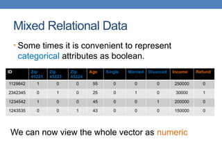
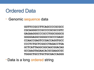
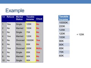
15. Examples
JSON EXAMPLE – Record of a person
{
"firstName": "John",
"lastName": "Smith",
"isAlive": true,
"age": 25,
"address": {
"streetAddress": "21 2nd Street",
"city": "New York",
"state": "NY",
"postalCode": "10021-3100"
},
"phoneNumbers": [
{
"type": "home",
"number": "212 555-1234"
},
{
"type": "office",
"number": "646 555-4567"
}
],
"children": [],
"spouse": null
}
XML EXAMPLE – Record of a person
<person>
<firstName>John</firstName>
<lastName>Smith</lastName>
<age>25</age>
<address>
<streetAddress>21 2nd Street</streetAddress>
<city>New York</city>
<state>NY</state>
<postalCode>10021</postalCode>
</address>
<phoneNumbers>
<phoneNumber>
<type>home</type>
<number>212 555-1234</number>
</phoneNumber>
<phoneNumber>
<type>fax</type>
<number>646 555-4567</number>
</phoneNumber>
</phoneNumbers>
<gender>
<type>male</type>
</gender>
</person>

16. Set data
• Each record is a set of items from a space of
possible items
• Example: Transaction data
• Also called market-basket data
TID Items
1 Bread, Coke, Milk
2 Beer, Bread
3 Beer, Coke, Diaper, Milk
4 Beer, Bread, Diaper, Milk
5 Coke, Diaper, Milk

17. Set data
• Each record is a set of items from a space of
possible items
• Example: Document data
• Also called bag-of-words representation
Doc Id Words
1 the, dog, followed, the, cat
2 the, cat, chased, the, cat
3 the, man, walked, the, dog

18. Vector representation of market-basket data
• Market-basket data can be represented, or thought
of, as numeric vector data
• The vector is defined over the set of all possible items
• The values are binary (the item appears or not in the set)
TID Items
1 Bread, Coke, Milk
2 Beer, Bread
3 Beer, Coke, Diaper, Milk
4 Beer, Bread, Diaper, Milk
5 Coke, Diaper, Milk
TID
Brea
d
Coke
Milk
Beer
Diape
r
1 1 1 1 0 0
2 1 0 0 1 0
3 0 1 1 1 1
4 1 0 1 1 1
5 0 1 1 0 1
Sparsity: Most entries are zero. Most baskets contain few items

19. Vector representation of document data
• Document data can be represented, or thought of,
as numeric vector data
• The vector is defined over the set of all possible words
• The values are the counts (number of times a word
appears in the document)
Doc
Id
the
dog
follow
s
cat
chase
s
man
walks
1 2 1 1 1 0 0 0
2 2 0 0 2 1 0 0
3 1 1 0 0 0 1 1
Doc Id Words
1 the, dog, follows, the, cat
2 the, cat, chases, the, cat
3 the, man, walks, the, dog
Sparsity: Most entries are zero. Most documents contain few of the words

20. Physical data storage
• Usually set data is stored in flat files
• One line per set
• I heard so many good things about this place so I was pretty juiced to try it. I'm
from Cali and I heard Shake Shack is comparable to IN-N-OUT and I gotta say, Shake
Shake wins hands down. Surprisingly, the line was short and we waited about 10 MIN.
to order. I ordered a regular cheeseburger, fries and a black/white shake. So
yummerz. I love the location too! It's in the middle of the city and the view is
breathtaking. Definitely one of my favorite places to eat in NYC.
• I'm from California and I must say, Shake Shack is better than IN-N-OUT, all day,
err'day.
0 1 2 3 4 5 6 7 8 9 10 11 12 13 14 15 16 17 18 19 20 21 22 23 24 25 26 27 28 29
30 31 32
33 34 35
36 37 38 39 40 41 42 43 44 45 46
38 39 47 48
38 39 48 49 50 51 52 53 54 55 56 57 58
32 41 59 60 61 62
3 39 48

21. Ordered Data
• Genomic sequence data
• Data is a long ordered string
GGTTCCGCCTTCAGCCCCGCGCC
CGCAGGGCCCGCCCCGCGCCGTC
GAGAAGGGCCCGCCTGGCGGGCG
GGGGGAGGCGGGGCCGCCCGAGC
CCAACCGAGTCCGACCAGGTGCC
CCCTCTGCTCGGCCTAGACCTGA
GCTCATTAGGCGGCAGCGGACAG
GCCAAGTAGAACACGCGAAGCGC
TGGGCTGCCTGCTGCGACCAGGG

22. Ordered Data
• Time series
• Sequence of ordered (over “time”) numeric values.

23. Graph Data
• Graph data: a collection of entities and their
pairwise relationships. Examples:
• Web pages and hyperlinks
• Facebook users and friendships
• The connections between brain neurons
In this case the data
consists of pairs:
Who links to whom
1
2
3
4
5

24. Representation
• Adjacency matrix
• Very sparse, very wasteful, but useful conceptually
1
2
3
4
5

















0
0
0
0
0
1
0
0
0
0
0
1
0
1
0
0
0
0
0
1
0
0
1
1
0
A

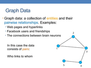
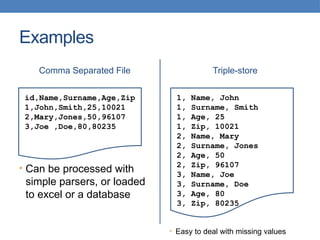
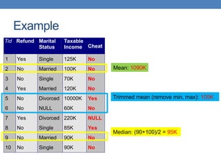
25. Representation
• Adjacency list
• Not so easy to maintain
1
2
3
4
5
1: [2, 3]
2: [1, 3]
3: [1, 2, 4]
4: [3, 5]
5: [4]

26. Representation
• List of pairs
• The simplest and most efficient representation
1
2
3
4
5
(1,2)
(2,3)
(1,3)
(3,4)
(4,5)

27. Types of data: summary
• Numeric data: Each object is a point in a
multidimensional space
• Categorical data: Each object is a vector of
categorical values
• Set data: Each object is a set of values (with or
without counts)
• Sets can also be represented as binary vectors, or
vectors of counts
• Ordered sequences: Each object is an ordered
sequence of values.
• Graph data: A collection of pairwise relationships

28. The data analysis pipeline
Data
Preprocessing
Data Mining
Result
Post-processing
Data
Collection
Mining is not the only step in the analysis process

29. The data analysis pipeline
• Today there is an abundance of data online
• Facebook, Twitter, Wikipedia, Web, City data, Open data initiatives, etc
• Collecting the data is a separate task
• Customized crawlers, use of public APIs
• Respect of crawling etiquette
• How should we store them?
• In many cases when collecting data we also need to label them
• E.g., how do we identify fraudulent transactions?
• E.g., how do we elicit user preferences?
Data
Preprocessing
Data Mining
Result
Post-processing
Data
Collection

30. The data analysis pipeline
Data
Preprocessing
Data Mining
Result
Post-processing
Data
Collection
• Preprocessing: Real data is large, noisy, incomplete and
inconsistent. Data cleaning is required to make sense of the
data
• Techniques: Sampling, Dimensionality Reduction, Feature selection.
• The preprocessing step determines the input to the data mining
algorithm
• A dirty work, but someone has to do it.
• It is often the most important step for the analysis

31. The data analysis pipeline
Data
Preprocessing
Data Mining
Result
Post-processing
Data
Collection
• Post-Processing: Make the data actionable and
useful to the user
• Statistical analysis of importance of results
• Visualization

32. The data analysis pipeline
Data
Preprocessing
Data Mining
Result
Post-processing
Data
Collection
Mining is not the only step in the analysis process
• Pre- and Post-processing are often data mining tasks as well

33. Data Quality
• Examples of data quality problems:
• Noise and outliers
• Missing values
• Duplicate data
Tid Refund Marital
Status
Taxable
Income Cheat
1 Yes Single 125K No
2 No Married 100K No
3 No Single 70K No
4 Yes Married 120K No
5 No Divorced 10000K Yes
6 No NULL 60K No
7 Yes Divorced 220K NULL
8 No Single 85K Yes
9 No Married 90K No
9 No Single 90K No
10
A mistake or a millionaire?
Missing values
Inconsistent duplicate entries

34. Sampling
• Sampling is the main technique employed for data selection.
• It is often used for both the preliminary investigation of the data and the
final data analysis.
• Statisticians sample because obtaining the entire set of data of
interest is too expensive or time consuming.
• Example: What is the average height of a person in Greece?
• We cannot measure the height of everybody
• Sampling is used in data mining because processing the entire
set of data of interest is too expensive or time consuming.
• Example: We have 1M documents. What fraction of pairs has at least 100
words in common?
• Computing number of common words for all pairs requires 1012
comparisons
• Example: What fraction of tweets in a year contain the word “Greece”?
• 500M tweets per day, if 100 characters on average, 86.5TB to store all tweets

35. Sampling …
• The key principle for effective sampling is the following:
• using a sample will work almost as well as using the entire
data sets, if the sample is representative
• A sample is representative if it has approximately the same
property (of interest) as the original set of data
• Otherwise we say that the sample introduces some bias
• What happens if we take a sample from the university campus
to compute the average height of a person at Ioannina?

36. Types of Sampling
• Simple Random Sampling
• There is an equal probability of selecting any particular item
• Sampling without replacement
• As each item is selected, it is removed from the population
• Sampling with replacement
• Objects are not removed from the population as they are selected for the
sample.
• In sampling with replacement, the same object can be picked up more than
once. This makes analytical computation of probabilities easier
• E.g., we have 100 people, 51 are women P(W) = 0.51, 49 men P(M) =
0.49. If I pick two persons what is the probability P(W,W) that both are
women?
• Sampling with replacement: P(W,W) = 0.512
• Sampling without replacement: P(W,W) = 51/100 * 50/99

37. Types of Sampling
• Stratified sampling
• Split the data into several groups; then draw random samples from each
group.
• Ensures that all groups are represented.
• Example 1. I want to understand the differences between legitimate and
fraudulent credit card transactions. 0.1% of transactions are fraudulent. What
happens if I select 1000 transactions at random?
• I get 1 fraudulent transaction (in expectation). Not enough to draw any conclusions. Solution:
sample 1000 legitimate and 1000 fraudulent transactions
• Example 2. I want to answer the question: Do web pages that are linked
have on average more words in common than those that are not? I have 1M
pages, and 1M links, what happens if I select 10K pairs of pages at random?
• Most likely I will not get any links. Solution: sample 10K random pairs, and 10K links
Probability Reminder: If an event has probability p of happening and I do N
trials, the expected number of times the event occurs is pN

38. Sample Size
8000 points 2000 Points 500 Points

39. Sample Size
• What sample size is necessary to get at least one
object from each of 10 groups.

40. A data mining challenge
• You have N items and you want to sample one item uniformly
at random. How do you do that?
• The items are coming in a stream: you do not know the size
of the stream in advance, and there is not enough memory to
store the stream in memory. You can only keep a constant
amount of items in memory
• How do you sample?
• Hint: if the stream ends after reading k items the last item in the
stream should have probability 1/k to be selected.
• Reservoir Sampling:
• Standard interview question for many companies

41. Reservoir sampling
• Algorithm: With probability 1/k select the k-th item of
the stream and replace the previous choice.
• Claim: Every item has probability 1/N to be selected
after N items have been read.
• Proof
• What is the probability of the k-th item to be selected?
• What is the probability of the n-th item to survive for N-n
rounds?

42. Proof by Induction
• We want to show that the probability the -th item is
selected after items have been seen is
• Induction on the number of steps
• Base of the induction: For , the probability that the -th item
is selected is
• Inductive Hypothesis: Assume that it is true for
• Inductive Step: The probability that the item is still
selected after items is

43. A data preprocessing example
• Suppose we want to mine the comments/reviews
of people on Yelp or Foursquare.

44. Mining Task
• Collect all reviews for the top-10 most reviewed
restaurants in NY in Yelp
• Find few terms that best describe the restaurants.
• Algorithm?
{"votes": {"funny": 0, "useful": 2, "cool": 1},
"user_id": "Xqd0DzHaiyRqVH3WRG7hzg",
"review_id": "15SdjuK7DmYqUAj6rjGowg",
"stars": 5, "date": "2007-05-17",
"text": "I heard so many good things about this place so I was pretty juiced to
try it. I'm from Cali and I heard Shake Shack is comparable to IN-N-OUT and I
gotta say, Shake Shake wins hands down. Surprisingly, the line was short and
we waited about 10 MIN. to order. I ordered a regular cheeseburger, fries and a
black/white shake. So yummerz. I love the location too! It's in the middle of
the city and the view is breathtaking. Definitely one of my favorite places to
eat in NYC.",
"type": "review",
"business_id": "vcNAWiLM4dR7D2nwwJ7nCA"}

45. Example data
• I heard so many good things about this place so I was pretty juiced to try it. I'm
from Cali and I heard Shake Shack is comparable to IN-N-OUT and I gotta say, Shake
Shake wins hands down. Surprisingly, the line was short and we waited about 10
MIN. to order. I ordered a regular cheeseburger, fries and a black/white shake. So
yummerz. I love the location too! It's in the middle of the city and the view is
breathtaking. Definitely one of my favorite places to eat in NYC.
• I'm from California and I must say, Shake Shack is better than IN-N-OUT, all day,
err'day.
• Would I pay $15+ for a burger here? No. But for the price point they are asking for,
this is a definite bang for your buck (though for some, the opportunity cost of
waiting in line might outweigh the cost savings) Thankfully, I came in before the
lunch swarm descended and I ordered a shake shack (the special burger with the patty
+ fried cheese &amp; portabella topping) and a coffee milk shake. The beef patty was
very juicy and snugly packed within a soft potato roll. On the downside, I could do
without the fried portabella-thingy, as the crispy taste conflicted with the juicy,
tender burger. How does shake shack compare with in-and-out or 5-guys? I say a very
close tie, and I think it comes down to personal affliations. On the shake side, true
to its name, the shake was well churned and very thick and luscious. The coffee
flavor added a tangy taste and complemented the vanilla shake well. Situated in an
open space in NYC, the open air sitting allows you to munch on your burger while
watching people zoom by around the city. It's an oddly calming experience, or perhaps
it was the food coma I was slowly falling into. Great place with food at a great
price.

46. First cut
• Do simple processing to “normalize” the data (remove punctuation, make
into lower case, clear white spaces, other?)
• Break into words, keep the most popular words
the 27514
and 14508
i 13088
a 12152
to 10672
of 8702
ramen 8518
was 8274
is 6835
it 6802
in 6402
for 6145
but 5254
that 4540
you 4366
with 4181
pork 4115
my 3841
this 3487
wait 3184
not 3016
we 2984
at 2980
on 2922
the 16710
and 9139
a 8583
i 8415
to 7003
in 5363
it 4606
of 4365
is 4340
burger 432
was 4070
for 3441
but 3284
shack 3278
shake 3172
that 3005
you 2985
my 2514
line 2389
this 2242
fries 2240
on 2204
are 2142
with 2095
the 16010
and 9504
i 7966
to 6524
a 6370
it 5169
of 5159
is 4519
sauce 4020
in 3951
this 3519
was 3453
for 3327
you 3220
that 2769
but 2590
food 2497
on 2350
my 2311
cart 2236
chicken 2220
with 2195
rice 2049
so 1825
the 14241
and 8237
a 8182
i 7001
to 6727
of 4874
you 4515
it 4308
is 4016
was 3791
pastrami 3748
in 3508
for 3424
sandwich 2928
that 2728
but 2715
on 2247
this 2099
my 2064
with 2040
not 1655
your 1622
so 1610
have 1585

47. First cut
• Do simple processing to “normalize” the data (remove punctuation, make
into lower case, clear white spaces, other?)
• Break into words, keep the most popular words
the 27514
and 14508
i 13088
a 12152
to 10672
of 8702
ramen 8518
was 8274
is 6835
it 6802
in 6402
for 6145
but 5254
that 4540
you 4366
with 4181
pork 4115
my 3841
this 3487
wait 3184
not 3016
we 2984
at 2980
on 2922
the 16710
and 9139
a 8583
i 8415
to 7003
in 5363
it 4606
of 4365
is 4340
burger 432
was 4070
for 3441
but 3284
shack 3278
shake 3172
that 3005
you 2985
my 2514
line 2389
this 2242
fries 2240
on 2204
are 2142
with 2095
the 16010
and 9504
i 7966
to 6524
a 6370
it 5169
of 5159
is 4519
sauce 4020
in 3951
this 3519
was 3453
for 3327
you 3220
that 2769
but 2590
food 2497
on 2350
my 2311
cart 2236
chicken 2220
with 2195
rice 2049
so 1825
the 14241
and 8237
a 8182
i 7001
to 6727
of 4874
you 4515
it 4308
is 4016
was 3791
pastrami 3748
in 3508
for 3424
sandwich 2928
that 2728
but 2715
on 2247
this 2099
my 2064
with 2040
not 1655
your 1622
so 1610
have 1585
Most frequent words are stop words

48. Second cut
• Remove stop words
• Stop-word lists can be found online.
a,about,above,after,again,against,all,am,an,and,any,are,aren't,as,at,be,be
cause,been,before,being,below,between,both,but,by,can't,cannot,could,could
n't,did,didn't,do,does,doesn't,doing,don't,down,during,each,few,for,from,f
urther,had,hadn't,has,hasn't,have,haven't,having,he,he'd,he'll,he's,her,he
re,here's,hers,herself,him,himself,his,how,how's,i,i'd,i'll,i'm,i've,if,in
,into,is,isn't,it,it's,its,itself,let's,me,more,most,mustn't,my,myself,no,
nor,not,of,off,on,once,only,or,other,ought,our,ours,ourselves,out,over,own
,same,shan't,she,she'd,she'll,she's,should,shouldn't,so,some,such,than,tha
t,that's,the,their,theirs,them,themselves,then,there,there's,these,they,th
ey'd,they'll,they're,they've,this,those,through,to,too,under,until,up,very
,was,wasn't,we,we'd,we'll,we're,we've,were,weren't,what,what's,when,when's
,where,where's,which,while,who,who's,whom,why,why's,with,won't,would,would
n't,you,you'd,you'll,you're,you've,your,yours,yourself,yourselves,

49. Second cut
• Remove stop words
• Stop-word lists can be found online.
ramen 8572
pork 4152
wait 3195
good 2867
place 2361
noodles 2279
ippudo 2261
buns 2251
broth 2041
like 1902
just 1896
get 1641
time 1613
one 1460
really 1437
go 1366
food 1296
bowl 1272
can 1256
great 1172
best 1167
burger 4340
shack 3291
shake 3221
line 2397
fries 2260
good 1920
burgers 1643
wait 1508
just 1412
cheese 1307
like 1204
food 1175
get 1162
place 1159
one 1118
long 1013
go 995
time 951
park 887
can 860
best 849
sauce 4023
food 2507
cart 2239
chicken 2238
rice 2052
hot 1835
white 1782
line 1755
good 1629
lamb 1422
halal 1343
just 1338
get 1332
one 1222
like 1096
place 1052
go 965
can 878
night 832
time 794
long 792
people 790
pastrami 3782
sandwich 2934
place 1480
good 1341
get 1251
katz's 1223
just 1214
like 1207
meat 1168
one 1071
deli 984
best 965
go 961
ticket 955
food 896
sandwiches 813
can 812
beef 768
order 720
pickles 699
time 662

50. Second cut
• Remove stop words
• Stop-word lists can be found online.
ramen 8572
pork 4152
wait 3195
good 2867
place 2361
noodles 2279
ippudo 2261
buns 2251
broth 2041
like 1902
just 1896
get 1641
time 1613
one 1460
really 1437
go 1366
food 1296
bowl 1272
can 1256
great 1172
best 1167
burger 4340
shack 3291
shake 3221
line 2397
fries 2260
good 1920
burgers 1643
wait 1508
just 1412
cheese 1307
like 1204
food 1175
get 1162
place 1159
one 1118
long 1013
go 995
time 951
park 887
can 860
best 849
sauce 4023
food 2507
cart 2239
chicken 2238
rice 2052
hot 1835
white 1782
line 1755
good 1629
lamb 1422
halal 1343
just 1338
get 1332
one 1222
like 1096
place 1052
go 965
can 878
night 832
time 794
long 792
people 790
pastrami 3782
sandwich 2934
place 1480
good 1341
get 1251
katz's 1223
just 1214
like 1207
meat 1168
one 1071
deli 984
best 965
go 961
ticket 955
food 896
sandwiches 813
can 812
beef 768
order 720
pickles 699
time 662
Commonly used words in reviews, not so interesting

51. IDF
• Important words are the ones that are unique to the document
(differentiating) compared to the rest of the collection
• All reviews use the word “like”. This is not interesting
• We want the words that characterize the specific restaurant
• Document Frequency : fraction of documents that contain word .
• Inverse Document Frequency :
• Maximum when unique to one document :
• Minimum when the word is common to all documents:
: num of docs that contain word
: total number of documents

52. TF-IDF
• The words that are best for describing a document are the
ones that are important for the document, but also unique
to the document.
• TF(w,d): term frequency of word w in document d
• Number of times that the word appears in the document
• Natural measure of importance of the word for the document
• IDF(w): inverse document frequency
• Natural measure of the uniqueness of the word w
• TF-IDF(w,d) = TF(w,d)  IDF(w)

53. Third cut
• Ordered by TF-IDF
ramen 3057.41761944282 7
akamaru 2353.24196503991 1
noodles 1579.68242449612 5
broth 1414.71339552285 5
miso 1252.60629058876 1
hirata 709.196208642166 1
hakata 591.76436889947 1
shiromaru 587.1591987134 1
noodle 581.844614740089 4
tonkotsu 529.594571388631 1
ippudo 504.527569521429 8
buns 502.296134008287 8
ippudo's 453.609263319827 1
modern 394.839162940177 7
egg 367.368005696771 5
shoyu 352.295519228089 1
chashu 347.690349042101 1
karaka 336.177423577131 1
kakuni 276.310211159286 1
ramens 262.494700601321 1
bun 236.512263803654 6
wasabi 232.366751234906 3
dama 221.048168927428 1
brulee 201.179739054263 2
fries 806.085373301536 7
custard 729.607519421517 3
shakes 628.473803858139 3
shroom 515.779060830666 1
burger 457.264637954966 9
crinkle 398.34722108797 1
burgers 366.624854809247 8
madison 350.939350307801 4
shackburger 292.428306810 1
'shroom 287.823136624256 1
portobello 239.8062489526 2
custards 211.837828555452 1
concrete 195.169925889195 4
bun 186.962178298353 6
milkshakes 174.9964670675 1
concretes 165.786126695571 1
portabello 163.4835416025 1
shack's 159.334353330976 2
patty 152.226035882265 6
ss 149.668031044613 1
patties 148.068287943937 2
cam 105.949606780682 3
milkshake 103.9720770839 5
lamps 99.011158998744 1
lamb 985.655290756243 5
halal 686.038812717726 6
53rd 375.685771863491 5
gyro 305.809092298788 3
pita 304.984759446376 5
cart 235.902194557873 9
platter 139.459903080044 7
chicken/lamb 135.8525204 1
carts 120.274374158359 8
hilton 84.2987473324223 4
lamb/chicken 82.8930633 1
yogurt 70.0078652365545 5
52nd 67.5963923222322 2
6th 60.7930175345658 9
4am 55.4517744447956 5
yellow 54.4470265206673 8
tzatziki 52.9594571388631 1
lettuce 51.3230168022683 8
sammy's 50.656872045869 1
sw 50.5668577816893 3
platters 49.9065970003161 5
falafel 49.4796995212044 4
sober 49.2211422635451 7
moma 48.1589121730374 3
pastrami 1931.94250908298 6
katz's 1120.62356508209 4
rye 1004.28925735888 2
corned 906.113544700399 2
pickles 640.487221580035 4
reuben 515.779060830666 1
matzo 430.583412389887 1
sally 428.110484707471 2
harry 226.323810772916 4
mustard 216.079238853014 6
cutter 209.535243462458 1
carnegie 198.655512713779 3
katz 194.387844446609 7
knish 184.206807439524 1
sandwiches 181.415707218 8
brisket 131.945865389878 4
fries 131.613054313392 7
salami 127.621117258549 3
knishes 124.339595021678 1
delicatessen 117.488967607 2
deli's 117.431839742696 1
carver 115.129254649702 1
brown's 109.441778045519 2
matzoh 108.22149937072 1

54. Third cut
• TF-IDF takes care of stop words as well
• We do not need to remove the stopwords since
they will get IDF(w) = 0

55. Decisions, decisions…
• When mining real data you often need to make some decisions
• What data should we collect? How much? For how long?
• Should we throw out some data that does not seem to be useful?
• Too frequent data (stop words), too infrequent (errors?), erroneous data, missing data, outliers
• How should we weight the different pieces of data?
• Most decisions are application dependent. Some information may be
lost but we can usually live with it (most of the times)
• We should make our decisions clear since they affect our findings.
• Dealing with real data is hard…
AAAAAAAAAAAAA
AAAAAAAAAAAAAAAAAAAAAAAAA AAAAAAAAAAAAAAAAAAAAAAAAA AAA
An actual review

56. Normalization
• In many cases it is important to normalize the
data rather than use the raw values
• In this data, different attributes take very different
range of values. For distance/similarity the small
values will disappear
• We need to make them comparable
Temperature Humidity Pressure
30 0.8 90
32 0.5 80
24 0.3 95

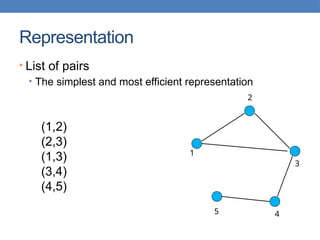
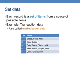
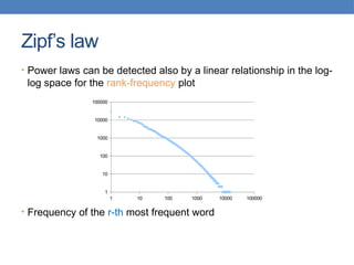
57. Normalization
• Divide (the values of a column) by the maximum
value for each attribute
• Brings everything in the [0,1] range
Temperature Humidity Pressure
0.9375 1 0.9473
1 0.625 0.8421
0.75 0.375 1
new value = old value / max value in the column
Temperature Humidity Pressure
30 0.8 90
32 0.5 80
24 0.3 95

58. Normalization
• Subtract the minimum value and divide by the
difference of the maximum value and minimum
value for each attribute
• Brings everything in the [0,1] range, minimum is zero
Temperature Humidity Pressure
0.75 1 0.33
1 0.6 0
0 0 1
new value = (old value – min column value) / (max col. value –min col. value)
Temperature Humidity Pressure
30 0.8 90
32 0.5 80
24 0.3 95

59. Normalization
• Are these documents similar?
Word 1 Word 2 Word 3
Doc 1 28 50 22
Doc 2 12 25 13

60. Normalization
• Are these documents similar?
• Divide by the sum of values for each document
(row in the matrix)
• Transform a vector into a distribution
Word 1 Word 2 Word 3
Doc 1 0.28 0.5 0.22
Doc 2 0.24 0.5 0.26
Word 1 Word 2 Word 3
Doc 1 28 50 22
Doc 2 12 25 13
new value = old value / Σ old values in the row

61. Normalization
• Do these two users rate movies in a similar way?
Movie 1 Movie 2 Movie 3
User 1 1 2 3
User 2 2 3 4

62. Normalization
• Do these two users rate movies in a similar way?
• Subtract the mean value for each user (row)
• Captures the deviation from the average behavior
Movie 1 Movie 2 Movie 3
User 1 -1 0 +1
User 2 -1 0 +1
Movie 1 Movie 2 Movie 3
User 1 1 2 3
User 2 2 3 4
new value = (old value – mean row value) [/ (max row value –min row value)]

63. Exploratory analysis of data
• Summary statistics: numbers that summarize
properties of the data
• Summarized properties include frequency, location and
spread
• Examples: location - mean
spread - standard deviation
• Most summary statistics can be calculated in a single
pass through the data

64. Frequency and Mode
• The frequency of an attribute value is the
percentage of time the value occurs in the
data set
• For example, given the attribute ‘gender’ and a
representative population of people, the gender ‘female’
occurs about 50% of the time.
• The mode of a an attribute is the most frequent
attribute value
• The notions of frequency and mode are typically
used with categorical data

65. Example
Tid Refund Marital
Status
Taxable
Income Cheat
1 Yes Single 125K No
2 No Married 100K No
3 No Single 70K No
4 Yes Married 120K No
5 No Divorced 10000K Yes
6 No NULL 60K No
7 Yes Divorced 220K NULL
8 No Single 85K Yes
9 No Married 90K No
10 No Single 90K No
10
Single Married Divorced NULL
4 3 2 1
Marital Status
Mode: Single

66. Example
Tid Refund Marital
Status
Taxable
Income Cheat
1 Yes Single 125K No
2 No Married 100K No
3 No Single 70K No
4 Yes Married 120K No
5 No Divorced 10000K Yes
6 No NULL 60K No
7 Yes Divorced 220K NULL
8 No Single 85K Yes
9 No Married 90K No
10 No Single 90K No
10
Marital Status
Single Married Divorced NULL
40% 30% 20% 10%

67. Example
Tid Refund Marital
Status
Taxable
Income Cheat
1 Yes Single 125K No
2 No Married 100K No
3 No Single 70K No
4 Yes Married 120K No
5 No Divorced 10000K Yes
6 No NULL 60K No
7 Yes Divorced 220K NULL
8 No Single 85K Yes
9 No Married 90K No
10 No Single 90K No
10
Marital Status
Single Married Divorced
44% 33% 22%

68. Percentiles
• For continuous data, the notion of a percentile is
more useful.
Given an ordinal or continuous attribute x and a
number p between 0 and 100, the pth
percentile is
a value of x such that p% of the observed values
of x are less or equal than .
• For instance, the 80th percentile is the value that
is greater or equal than 80% of all the values of x
we have in our data.

69. Example
Tid Refund Marital
Status
Taxable
Income Cheat
1 Yes Single 125K No
2 No Married 100K No
3 No Single 70K No
4 Yes Married 120K No
5 No Divorced 10000K Yes
6 No NULL 60K No
7 Yes Divorced 220K NULL
8 No Single 85K Yes
9 No Married 90K No
10 No Single 90K No
10
Taxable
Income
10000K
220K
125K
120K
100K
90K
90K
85K
70K
60K
= 125K

70. Measures of Location: Mean and Median
• The mean is the most common measure of the
location of a set of points.
• However, the mean is very sensitive to outliers.
• Thus, the median or a trimmed mean is also
commonly used.

71. Example
Tid Refund Marital
Status
Taxable
Income Cheat
1 Yes Single 125K No
2 No Married 100K No
3 No Single 70K No
4 Yes Married 120K No
5 No Divorced 10000K Yes
6 No NULL 60K No
7 Yes Divorced 220K NULL
8 No Single 85K Yes
9 No Married 90K No
10 No Single 90K No
10
Mean: 1090K
Trimmed mean (remove min, max): 105K
Median: (90+100)/2 = 95K

72. Measures of Spread: Range and Variance
• Range is the difference between the max and min
• The variance or standard deviation is the most
common measure of the spread of a set of points.

73. Normal Distribution
•
• An important distribution that characterizes many
quantities and has a central role in probabilities and
statistics.
• Appears also in the central limit theorem
• Fully characterized by the mean and standard
deviation
This is a value histogram

74. Not everything is normally distributed
• Plot of number of words with x number of occurrences
• If this was a normal distribution we would not have a
frequency as large as 28K
0 5000 10000 15000 20000 25000 30000 35000
0
1000
2000
3000
4000
5000
6000
7000
8000

75. Power-law distribution
• We can understand the distribution of words if we take
the log-log plot
• Linear relationship in the log-log space
1 10 100 1000 10000 100000
1
10
100
1000
10000
The slope of the
line gives us the
exponent α

76. Power-laws are everywhere
• Incoming and outgoing links of web pages, number of friends in
social networks, number of occurrences of words, file sizes, city
sizes, income distribution, popularity of products and movies
• Signature of human activity?
• A mechanism that explains everything?
• Rich get richer process

77. Zipf’s law
• Power laws can be detected also by a linear relationship in the log-
log space for the rank-frequency plot
• Frequency of the r-th most frequent word
1 10 100 1000 10000 100000
1
10
100
1000
10000
100000

78. The importance of correct representation
• Consider the following three plots which are histograms of
values. What do you observe? What can you tell of the
underlying function?
0 10 20 30 40 50 60 70 80 90 100
0
0.1
0.2
0.3
0.4
0.5
0.6
0.7
0.8
0 10 20 30 40 50 60 70 80 90 100
0
0.05
0.1
0.15
0.2
0.25
0.3
0.35
0.4
0 10 20 30 40 50 60 70 80 90 100
0
0.1
0.2
0.3
0.4
0.5
0.6
0.7
0.8
0.9
1

79. The importance of correct representation
• Putting all three plots together makes it more clear to see
the differences
• Green falls more slowly. Blue and Red seem more or less
the same
0 10 20 30 40 50 60 70 80 90 100
0
0.1
0.2
0.3
0.4
0.5
0.6
0.7
0.8
0.9
1
Series1
Series3
Series5

80. The importance of correct representation
• Making the plot in log-log space makes the differences more clear
• Green and Blue form straight lines. Red drops exponentially.
•
•
•
1 10 100
1E-30
1E-27
1E-24
1E-21
1E-18
1E-15
1E-12
0.000000001
0.000001
0.001
1
Series1
Series3
Series5
Linear relationship in log-log
means polynomial in linear-linear
The slope in the log-log is the
exponent of the polynomial

81. Scatter Plot Array of Iris Attributes
What do you see in these plots? Correlations Class Separation

82. Post-processing
• Visualization
• The human eye is a powerful analytical tool
• If we visualize the data properly, we can discover
patterns and demonstrate trends
• Visualization is the way to present the data so that
patterns can be seen
• E.g., histograms and plots are a form of visualization
• There are multiple techniques (a field on its own)

83. Visualization on a map
• John Snow, London 1854

84. Dimensionality Reduction
• The human eye is limited to processing
visualizations in two (at most three) dimensions
• One of the great challenges in visualization is to
visualize high-dimensional data into a two-
dimensional space
• Dimensionality reduction
• Distance preserving embeddings

85. Charles Minard map
Six types of data in one plot: size of
army, temperature, direction, location,
dates etc

86. Word Clouds
• A fancy way to visualize a document or collection
of documents.

87. Heatmaps
• Plot a point-to-point similarity matrix using a heatmap:
• Deep red = high values (hot)
• Dark blue = low values (cold)
0 0.2 0.4 0.6 0.8 1
0
0.1
0.2
0.3
0.4
0.5
0.6
0.7
0.8
0.9
1
x
y
Points
Points
20 40 60 80 100
10
20
30
40
50
60
70
80
90
100
Similarity
0
0.1
0.2
0.3
0.4
0.5
0.6
0.7
0.8
0.9
1
The clustering structure becomes clear in the heatmap

88. Heatmaps
• Heatmap (grey scale) of the data matrix
• Document-word frequencies
Documents
Words
Before clustering After clustering

89. Heatmaps
A very popular way to visualize data
http://projects.oregonlive.com/ucc-shooting/gun-deaths.php

90. Statistical Significance
• When we extract knowledge from a large dataset we need
to make sure that what we found is not an artifact of
randomness
• E.g., we find that many people buy milk and toilet paper together.
• But many (more) people buy milk and toilet paper independently
• Statistical tests compare the results of an experiment with
those generated by a null hypothesis
• E.g., a null hypothesis is that people select items independently.
• A result is interesting if it cannot be produced by
randomness.
• An important problem is to define the null hypothesis correctly:
What is random?

91. 91
Meaningfulness of Answers
• A big data-mining risk is that you will “discover”
patterns that are meaningless.
• Statisticians call it Bonferroni’s principle:
(roughly) if you look in more places for
interesting patterns than your amount of data
will support, you are bound to find crap.
• The Rhine Paradox: a great example of how
not to conduct scientific research.
CS345A Data Mining on the Web: Anand Rajaraman, Jeff Ullman

92. 92
Rhine Paradox – (1)
• Joseph Rhine was a parapsychologist in the
1950’s who hypothesized that some people had
Extra-Sensory Perception.
• He devised (something like) an experiment where
subjects were asked to guess 10 hidden cards –
red or blue.
• He discovered that almost 1 in 1000 had ESP –
they were able to get all 10 right!
CS345A Data Mining on the Web: Anand Rajaraman, Jeff Ullman

93. 93
Rhine Paradox – (2)
• He told these people they had ESP and called
them in for another test of the same type.
• Alas, he discovered that almost all of them had
lost their ESP.
• Why?
• What did he conclude?
• Answer on next slide.
CS345A Data Mining on the Web: Anand Rajaraman, Jeff Ullman

94. 94
Rhine Paradox – (3)
• He concluded that you shouldn’t tell people they
have ESP; it causes them to lose it.
CS345A Data Mining on the Web: Anand Rajaraman, Jeff Ullman