Basic Data Structures

1. Introduction:
Basic Concepts and Notations
Complexity analysis: time space tradeoff
Algorithmic notations, Big O notation
Introduction to omega, theta and little o
notation

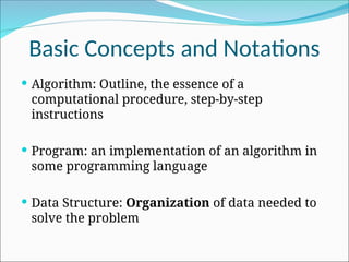
2. Basic Concepts and Notations
 Algorithm: Outline, the essence of a
computational procedure, step-by-step
instructions
 Program: an implementation of an algorithm in
some programming language
 Data Structure: Organization of data needed to
solve the problem

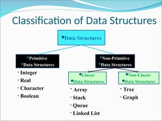
3. Classification of Data Structures
Data Structures
Primitive
Data Structures
Non-Primitive
Data Structures
Linear
Data Structures
Non-Linear
Data Structures
• Integer
• Real
• Character
• Boolean
• Array
• Stack
• Queue
• Linked List
• Tree
• Graph

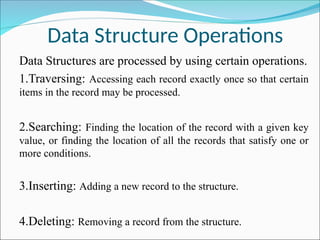
4. Data Structure Operations
Data Structures are processed by using certain operations.
1.Traversing: Accessing each record exactly once so that certain
items in the record may be processed.
2.Searching: Finding the location of the record with a given key
value, or finding the location of all the records that satisfy one or
more conditions.
3.Inserting: Adding a new record to the structure.
4.Deleting: Removing a record from the structure.

5. Special Data Structure-
Operations
• Sorting: Arranging the records in some logical order
(Alphabetical or numerical order).
• Merging: Combining the records in two different sorted
files into a single sorted file.

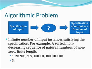
6. Algorithmic Problem
 Infinite number of input instances satisfying the
specification. For example: A sorted, non-
decreasing sequence of natural numbers of non-
zero, finite length:
 1, 20, 908, 909, 100000, 1000000000.
 3.
Specification
of input ?
Specification
of output as a
function of
input

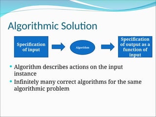
7. Algorithmic Solution
 Algorithm describes actions on the input
instance
 Infinitely many correct algorithms for the same
algorithmic problem
Specification
of input
Algorithm
Specification
of output as a
function of
input

8. What is a Good Algorithm?
 Efficient:
 Running time
 Space used
 Efficiency as a function of input size:
 The number of bits in an input number
 Number of data elements(numbers, points)

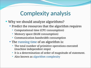
9. Complexity analysis
 Why we should analyze algorithms?
 Predict the resources that the algorithm requires
 Computational time (CPU consumption)
 Memory space (RAM consumption)
 Communication bandwidth consumption
 The running time of an algorithm is:
 The total number of primitive operations executed
(machine independent steps)
 It is a determination of order of magnitude of statement.
 Also known as algorithm complexity

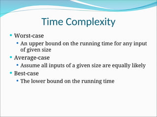
10. Time Complexity
 Worst-case
 An upper bound on the running time for any input
of given size
 Average-case
 Assume all inputs of a given size are equally likely
 Best-case
 The lower bound on the running time

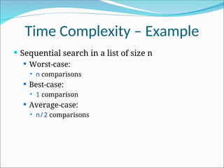
11. Time Complexity – Example
 Sequential search in a list of size n
 Worst-case:
 n comparisons
 Best-case:
 1 comparison
 Average-case:
 n/2 comparisons

12. time space tradeoff
 A time space tradeoff is a situation where the
memory use can be reduced at the cost of slower
program execution (and, conversely, the
computation time can be reduced at the cost of
increased memory use).
 A space-time or time-memory tradeoff is a way of
solving a problem or calculation in less time by using
more storage space (or memory), or by solving a
problem in very little space by spending a long time.

13. time space tradeoff
 As the relative costs of CPU cycles, RAM space, and
hard drive space change—hard drive space has for
some time been getting cheaper at a much faster rate
than other components of computers—the
appropriate choices for time space tradeoff have
changed radically.
 Often, by exploiting a time space tradeoff, a program
can be made to run much faster.

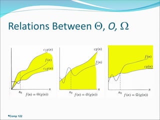
14. Asymptotic notations
 Algorithm complexity is rough estimation of
the number of steps performed by given
computation depending on the size of the
input data
 Measured through asymptotic notation
 O(g) where g is a function of the input data
size
 Examples:
 Linear complexity O(n) – all elements are processed once
(or constant number of times)
 Quadratic complexity O(n2
) – each of the elements is
processed n times

15. Big-O Notation (O)
Asymptotic Upper Bound

18. Omega Notation (Ω)
Asymptotic Lower Bound

20. Theta Notation (Θ)
g(n) is an asymptotically tight bound of f(n)

23. little o notation

24. ω-notation

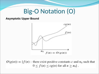
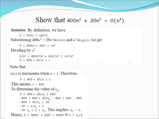
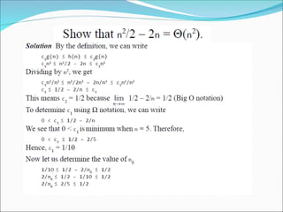
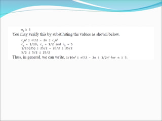
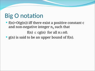
25. Big O notation
 f(n)=O(g(n)) iff there exist a positive constant c
and non-negative integer n0 such that
f(n)  cg(n) for all nn0.
 g(n) is said to be an upper bound of f(n).

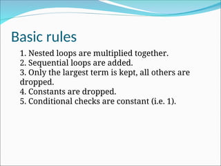
26. Basic rules
1. Nested loops are multiplied together.
2. Sequential loops are added.
3. Only the largest term is kept, all others are
dropped.
4. Constants are dropped.
5. Conditional checks are constant (i.e. 1).

27. Example 1
 //linear
 for(int i = 0; i < n; i++) {
 cout << i << endl;
 }

28.  Ans: O(n)

29. Example 2
 //quadratic
 for(int i = 0; i < n; i++) {
 for(int j = 0; j < n; j++){
 //do swap stuff, constant time
 }
 }

30.  Ans O(n^2)

31. Example 3
 for(int i = 0; i < 2*n; i++) {
 cout << i << endl;
 }

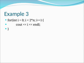
32.  At first you might say that the upper bound is
O(2n); however, we drop constants so it becomes
O(n)

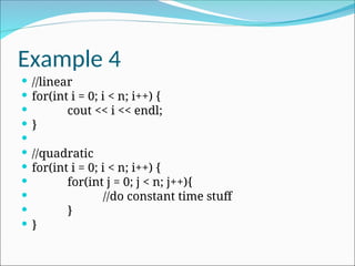
33. Example 4
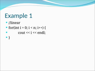
 //linear
 for(int i = 0; i < n; i++) {
 cout << i << endl;
 }

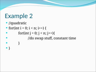
 //quadratic
 for(int i = 0; i < n; i++) {
 for(int j = 0; j < n; j++){
 //do constant time stuff
 }
 }

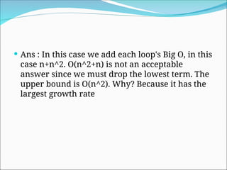
34.  Ans : In this case we add each loop's Big O, in this
case n+n^2. O(n^2+n) is not an acceptable
answer since we must drop the lowest term. The
upper bound is O(n^2). Why? Because it has the
largest growth rate

35. Example 5
 for(int i = 0; i < n; i++) {
 for(int j = 0; j < 2; j++){
 //do stuff
 }
 }

36.  Ans: Outer loop is 'n', inner loop is 2, this we
have 2n, dropped constant gives up O(n)

37. Example 6
x=y+z;
for(i=1; i<= n; i++)
x=y+z;
for(i=1; i<=n/2; i++)
for(j=1; j<=n; j++)
x=y+z;

38. Example 7
x=y+z;
for(i=1; i<= n; i++)
x=y+z;
for(i=1; i<=n; i++)
for(j=1; j<=n; j++)
x=y+z;
a=b+c;

39. Example 8
while(n>1)
{
n=n-1;
a=b+c;
}

40. Example 10
while(n>=1)
{
n=n-20;
n=n-5;
n=n-2;
}

41. Example 11
while(n>=1)
{
n=n-20;
n=n+5;
n=n-30;
}

42. Example 12
while(n>=1)
{
n=n/2;
}

43. Example 13
while(n>=1)
{
n=n/2;
n=n/3;
}

44. Example 14
while(n>=1)
{
n=n-2;
n=n/2;
}

45. Example 15
 for(int i = 1; i < n; i *= 2) {
 cout << i << endl;
 }

46.  There are n iterations, however, instead of
simply incrementing, 'i' is increased by 2*itself
each run. Thus the loop is log(n).

47. Example 16
 for(int i = 0; i < n; i++) { //linear
 for(int j = 1; j < n; j *= 2){ // log (n)
 //do constant time stuff
 }
 }

48.  Ans: n*log(n)

49. Example 17
while(n>2)
{
n=√n;
}

50. Example 18
while(n>2)
{
n=n2;
n=√n;
n=n-2;
}

51. Example 19
x=y+z;
for(i=1; i<= n; i++)
{
j=2;
while(j<=n)
{
j=j2;
}
}

52. Comp 122

53. Thank You