This document contains notes from the MIT course 6.851 (Advanced Data Structures) taught in Spring 2012 and previous years. It covers various topics in data structures, including temporal data structures, geometric data structures, dynamic optimality, memory hierarchies, dictionaries, integer data structures, and static trees. The notes are organized into 15 sections, each covering a different lecture and containing summaries provided by multiple student scribes.
![8.1 From Last Lectures. . . . . . . . . . . . . . . . . . . . . . . . . . . . . . . . . . . . . . 67
8.2 Ordered File Maintenance [55] [56] . . . . . . . . . . . . . . . . . . . . . . . . . . . . 67
8.3 List Labeling . . . . . . . . . . . . . . . . . . . . . . . . . . . . . . . . . . . . . . . . 70
8.4 Cache-Oblivious Priority Queues [59] . . . . . . . . . . . . . . . . . . . . . . . . . . . 70
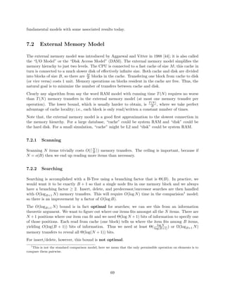
9 9. Memory hierarchy 3 73
Scribers: Tim Kaler(2012), Jenny Li(2012), Elena Tatarchenko(2012)
9.1 Overview . . . . . . . . . . . . . . . . . . . . . . . . . . . . . . . . . . . . . . . . . . 73
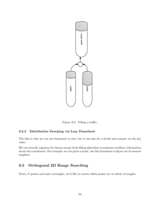
9.2 Lazy Funnelsort . . . . . . . . . . . . . . . . . . . . . . . . . . . . . . . . . . . . . . . 73
9.3 Orthogonal 2D Range Searching . . . . . . . . . . . . . . . . . . . . . . . . . . . . . 75
10 10. Dictionaries 82
Scribers: Edward Z. Yang (2012), Katherine Fang (2012), Benjamin Y. Lee
(2012), David Wilson (2010), Rishi Gupta (2010)
10.1 Overview . . . . . . . . . . . . . . . . . . . . . . . . . . . . . . . . . . . . . . . . . . 82
10.2 Hash Function . . . . . . . . . . . . . . . . . . . . . . . . . . . . . . . . . . . . . . . 82
10.3 Basic Chaining . . . . . . . . . . . . . . . . . . . . . . . . . . . . . . . . . . . . . . . 84
10.4 FKS Perfect Hashing { Fredman, Komlos, Szemeredi (1984) [157] . . . . . . . . . . . 86
10.5 Linear probing . . . . . . . . . . . . . . . . . . . . . . . . . . . . . . . . . . . . . . . 87
10.6 Cuckoo Hashing { Pagh and Rodler (2004) [155] . . . . . . . . . . . . . . . . . . . . 88
11 11. Integer 1 92
Scribers: Sam Fingeret (2012), Shravas Rao (2012), Paul Christiano (2010)
11.1 Overview . . . . . . . . . . . . . . . . . . . . . . . . . . . . . . . . . . . . . . . . . . 92
11.2 Integer Data Structures . . . . . . . . . . . . . . . . . . . . . . . . . . . . . . . . . . 92
11.3 Successor / Predecessor Queries . . . . . . . . . . . . . . . . . . . . . . . . . . . . . . 93
11.4 Van Emde Boas Trees . . . . . . . . . . . . . . . . . . . . . . . . . . . . . . . . . . . 94
11.5 Binary tree view . . . . . . . . . . . . . . . . . . . . . . . . . . . . . . . . . . . . . . 95
11.6 Reducing space . . . . . . . . . . . . . . . . . . . . . . . . . . . . . . . . . . . . . . . 96
12 12. Integer 2 98](https://image.slidesharecdn.com/datastructures-140901161631-phpapp02/85/Data-structures-5-320.jpg)
![sh (2003)
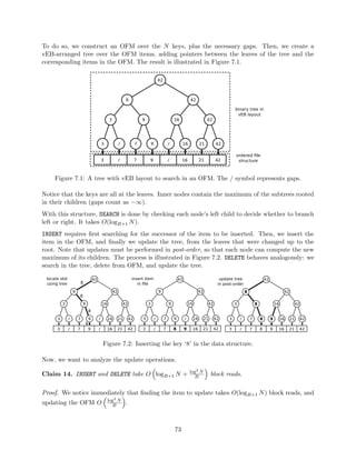
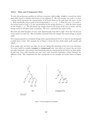
16.1 Overview . . . . . . . . . . . . . . . . . . . . . . . . . . . . . . . . . . . . . . . . . . 128
16.2 Predecessor Problem . . . . . . . . . . . . . . . . . . . . . . . . . . . . . . . . . . . . 128
16.3 Sux Trees . . . . . . . . . . . . . . . . . . . . . . . . . . . . . . . . . . . . . . . . . 132
16.4 Sux Arrays . . . . . . . . . . . . . . . . . . . . . . . . . . . . . . . . . . . . . . . . 134
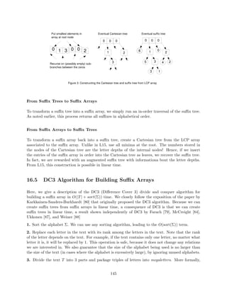
16.5 DC3 Algorithm for Building Sux Arrays . . . . . . . . . . . . . . . . . . . . . . . . 136
17 17. Succinct 1 139
Scribers: David Benjamin(2012), Lin Fei(2012), Yuzhi Zheng(2012),Morteza
Zadimoghaddam(2010), Aaron Bernstein(2007)
17.1 Overview . . . . . . . . . . . . . . . . . . . . . . . . . . . . . . . . . . . . . . . . . . 139
17.2 Level Order Representation of Binary Tries . . . . . . . . . . . . . . . . . . . . . . . 141
17.3 Rank and Select . . . . . . . . . . . . . . . . . . . . . . . . . . . . . . . . . . . . . . 143
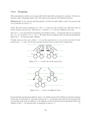
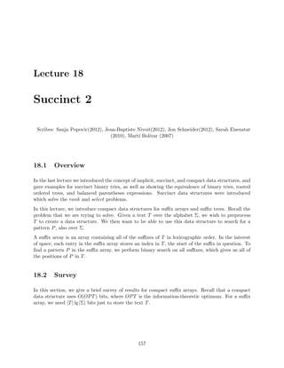
17.4 Subtree Sizes . . . . . . . . . . . . . . . . . . . . . . . . . . . . . . . . . . . . . . . . 146
18 18. Succinct 2 148
Scribers: Sanja Popovic(2012), Jean-Baptiste Nivoit(2012), Jon Schneider(2012),
Sarah Eisenstat (2010), Mart Bolvar (2007)
18.1 Overview . . . . . . . . . . . . . . . . . . . . . . . . . . . . . . . . . . . . . . . . . . 148
18.2 Survey . . . . . . . . . . . . . . . . . . . . . . . . . . . . . . . . . . . . . . . . . . . . 148
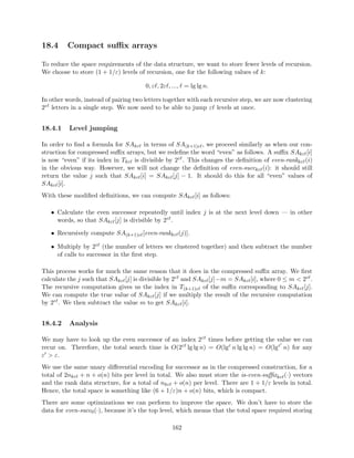
18.3 Compressed sux arrays . . . . . . . . . . . . . . . . . . . . . . . . . . . . . . . . . . 150
18.4 Compact sux arrays . . . . . . . . . . . . . . . . . . . . . . . . . . . . . . . . . . . 153
18.5 Sux trees [99] . . . . . . . . . . . . . . . . . . . . . . . . . . . . . . . . . . . . . . . 154
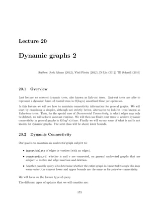
19 19. Dynamic graphs 1 157
Scribers: Justin Holmgren (2012), Jing Jian (2012), Maksim Stepanenko (2012),
Mashhood Ishaque (2007)](https://image.slidesharecdn.com/datastructures-140901161631-phpapp02/85/Data-structures-9-320.jpg)
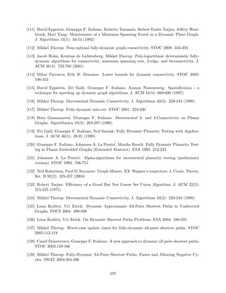
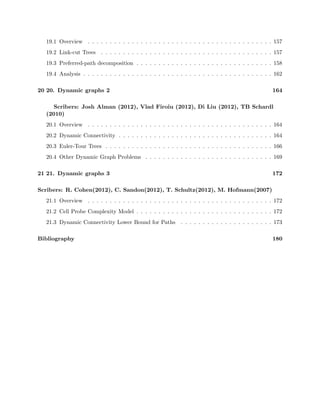
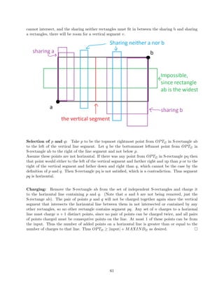
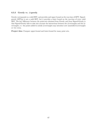
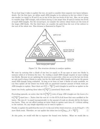
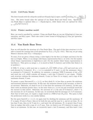
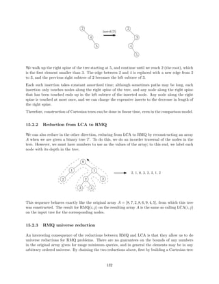
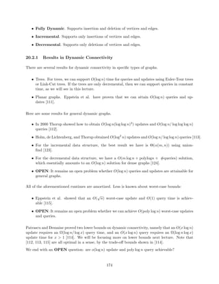
![nition implies a linear ordering on
the versions like in 1.1a.
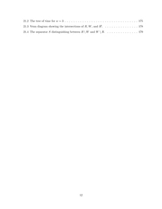
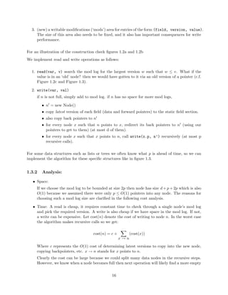
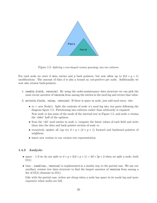
2. Full Persistence { In this model, both updates and queries are allowed on any version of the
data structure. We have operations read(var, version) and newversion = write(var,
version, val). The versions form a branching tree as in 1.1b.
3. Con
uent Persistence { In this model, in addition to the previous operation, we allow combi-nation
operations to combine input of more than one previous versions to output a new single
version. We have operations read(var, version), newversion = write(var, version,
val) and newversion = combine(var, val, version1, version2). Rather than a branch-ing
tree, combinations of versions induce a DAG (direct acyclic graph) structure on the version
graph, shown in 1.1c
4. Functional Persistence { This model takes its name from functional programming where
objects are immutable. The nodes in this model are likewise immutable: revisions do not
alter the existing nodes in the data structure but create new ones instead. Okasaki discusses
these as well as other functional data structures in his book [10].
The dierence between functional persistence and the rest is we have to keep all the structures
related to previous versions intact: the only allowed internal operation is to add new nodes. In the
previous three cases we were allowed anything as long as we were able to implement the interface.
Each of the succeeding levels of persistence is stronger than the preceding ones. Functional implies
con
uent, con
uent implies full, and full implies partial.
Functional implies con
uent because we are simply restricting ways on how we implement persis-tence.
Con
uent persistence becomes full persistence if we restrict ourselves to not use combinators.
And full persistence becomes partial when we restrict ourselves to only write to the latest version.
14](https://image.slidesharecdn.com/datastructures-140901161631-phpapp02/85/Data-structures-31-320.jpg)
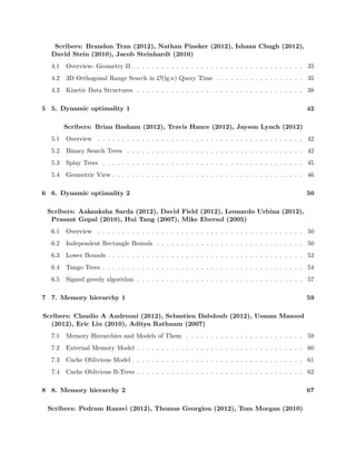
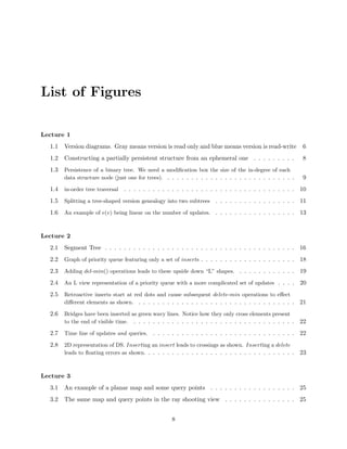
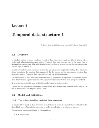
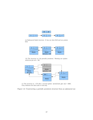
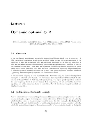
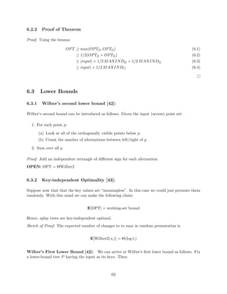
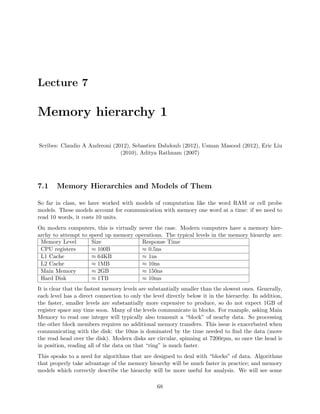
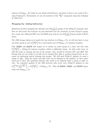
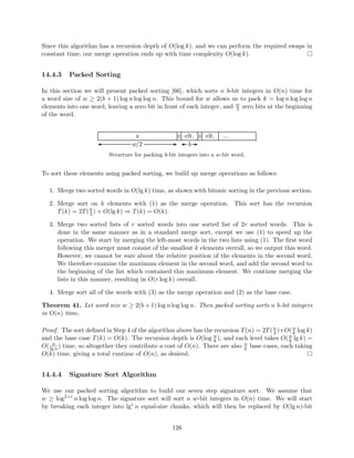
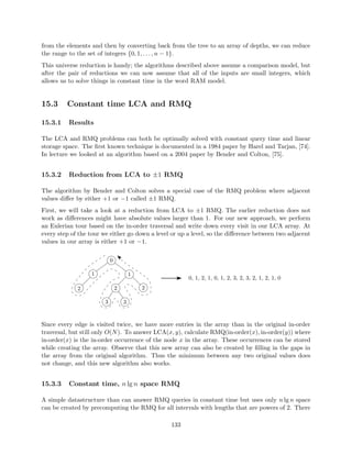
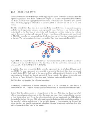
![nition.
(a) Partial. (b) Full
(c) Con
uent/ Functional
Figure 1.1: Version diagrams. Gray means version is read only and blue means version is read-write
1.3 Partial persistence
Question: Is it possible to implement partial persistence eciently?
Answer: Yes, assuming the pointer machine memory model and the restricting in-degrees of data
nodes to be O(1). This result is due to Driscoll, Sarnak, Sleator, and Tarjan [6].
Proof idea: We will expand our data nodes to keep a modi](https://image.slidesharecdn.com/datastructures-140901161631-phpapp02/85/Data-structures-33-320.jpg)

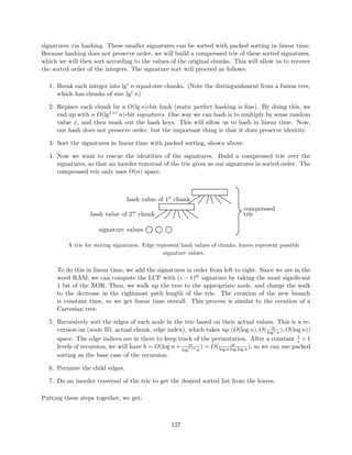
![cation box the size of the in-degree of each data
structure node (just one for trees).
mod log. For that reason amortized analysis more appropriate for this operation than worst
case analysis.
Recall the potential method technique explained in [68]: if we know a potential function ,
then amortized cost(n) = cost(n) + .
Consider the following potential function:
= c # mod log entries in current data nodes
Since the node was full and now it is empty, the change in potential associated with our new
node is 2cp. So now we can write a recursive expression for our amortized cost:
amortized cost(n) c + c 2cp + p amortized cost(x)
For some worst case node x. The second c covers the case where we](https://image.slidesharecdn.com/datastructures-140901161631-phpapp02/85/Data-structures-51-320.jpg)
![nish despite potential cycles in the graph, because splits decrease
and is non-negative.
Further study by Brodal [1] has shown actual cost to also be O(1) in the worst case.
1.4 Full persistence
The construction for partial persistence can be expanded to implement full persistence. This result
is also due to [6]. We again assume a pointer machine with p O(1) incoming pointers per node.
We need to take care of a two new problems:
1) Now we need to represent versions in a way that lets us eciently check which precedes which.
Versions form a tree, but traversing it is O(# of versions).
18](https://image.slidesharecdn.com/datastructures-140901161631-phpapp02/85/Data-structures-53-320.jpg)
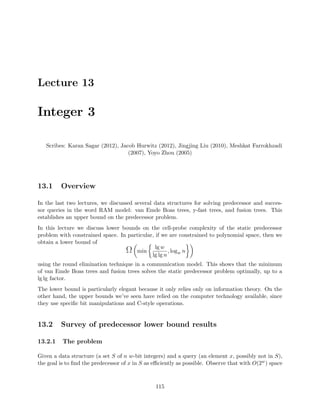
![ed element.
check if item s precedes item t.
For example, a linked list supports insertions in O(1), but tests for precedence take O(n). Similarly,
a balanced BST supports both operations but in O(log n) time. Deitz and Sleator show an O(1)
implementation for both operations in [4], which will be covered in lecture 8.
To implement version tree queries such as `is version v an ancestor of version w' we can use two
comparison queries bv bw and ew ev in O(1). To implement updates like `add version v as a
child of version w' we can insert the two elements bv and ev after bw and before ew respectively,
also in O(1).
1.4.2 Construction and algorithm:
The nodes in our data structure will keep the same kinds of additional data per node as they did
in the partially persistent case.
19](https://image.slidesharecdn.com/datastructures-140901161631-phpapp02/85/Data-structures-56-320.jpg)
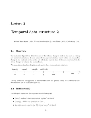
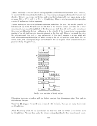
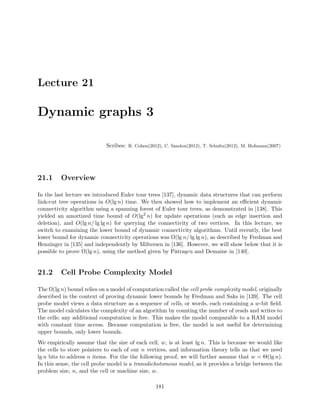
![gure 1.6.
Deques (double ended queues allowing stack and queue operations) with concatenation can be done
in constant time per operation (Kaplan, Okasaki, and Tarjan [8]). Like with a string, we can create
implicitly exponential deques in polynomial time by recursively concatenating a deque with itself.
The general transformation due to Fiat and Kaplan [9] is as follows:
e(v) = 1 + log(# of paths from root to v). This measure is called the `eective depth' of the
version DAG: if we unravel the tree via a DFS (by making a copy of each path as if they
didn't overlap) and rebalanced that tree this is the best we could hope to achieve.
d(v) = depth of node v in version DAG
overhead: log(# of updates) + maxv(e(v))
This results re
ects poor performance when e(v) = 2u where u is the number of updates. This is
still exponentially better than the complete copy.
A lower bound also by Fiat and Kaplan is
(e(v)) for update if queries are free. Their construction
makes e(v) queries per update.
OPEN: O(1) or even O(log (n)) space overhead per operation.
Collette, Iacono and Langerman consider the special case of `disjoint operations': con
uent opera-tions
performed only between versions with no shared data nodes. From there they show O(log (n))
overhead is possible for that case.
If we only allow disjoint operations, then each data node's version history is a tree. When evaluating
read(node, field, version) there are tree cases: when node modi](https://image.slidesharecdn.com/datastructures-140901161631-phpapp02/85/Data-structures-65-320.jpg)
![cation. This problem can be solved with use of `link-cut trees' (see lecture 19). Finally, when
version is below a leaf the problem is more complicated. The proof makes use of techniques such
as fractional cascading which will be covered in lecture 3. The full construction is explained in [11].
21](https://image.slidesharecdn.com/datastructures-140901161631-phpapp02/85/Data-structures-70-320.jpg)
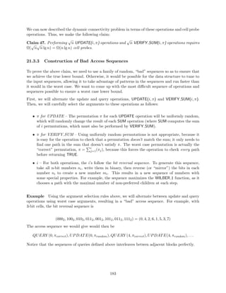
![Figure 1.6: An example of e(v) being linear on the number of updates.
1.6 Functional persistence
Functional persistence and data structures are explored in [10]. Simple examples of existing tech-niques
include the following.
Functional balanced BSTs { to persist BST's functionally, the main idea (a.k.a. `Path copy-ing')
is to duplicate the modi](https://image.slidesharecdn.com/datastructures-140901161631-phpapp02/85/Data-structures-71-320.jpg)
![ed node and propagate pointer changes by duplicating all
ancestors. If there are no parent pointers, work top down. This technique has an overhead
of O(log (n)) per operation, assuming the tree is balanced. Demaine, Langerman, Price show
this for link-cut trees as well [3].
Deques { (double ended queues allowing stack and queue operations) with concatenation can
be done in constant time per operation (Kaplan, Okasaki, and Tarjan [8]). Furthermore,
Brodal, Makris and Tsichlas show in [14] it can be done with concatenation in constant time
and update and search in O(log (n))
Tries { with local navigation and subtree copy and delete. Demaine, Langerman, Price show
how to persist this structure optimally in [3].
Pippenger shows at most log () cost separation of the functional version from the regular data
structure in [13].
OPEN: (for both functional and con
uent) bigger separation? more general structure transforma-tions?
OPEN: Lists with split and concatenate? General pointer machine?
OPEN: Array with cut and paste? Special DAGs?
22](https://image.slidesharecdn.com/datastructures-140901161631-phpapp02/85/Data-structures-72-320.jpg)
![es DS, we must
say which future queries are changed.
2.2.1 Easy case with commutativity and inversions
Assume the following hold:
Commutative updates: x:y = y:x (x followed by y is the same as y followed by x); that is the
updates can be reordered ) Insert(t, op) = Insert(now, op).
Invertible updates: There exists an operation x1, such that x:x1 = ; ) Delete(t, op) =
Insert(now, op1)
Partial retroactivity
These two assumptions allow us to solve some retroactive problems easily, such as:
hashing
array with operation A[i]+ = (but no direct assignment)
2.2.2 Full retroactivity
First, lets de](https://image.slidesharecdn.com/datastructures-140901161631-phpapp02/85/Data-structures-77-320.jpg)
![ne the search problem: maintain set S of objects, subject to insert, delete,
query(x; S).
Decomposable search problem [1980, 2007]: same as the search problem, with a restriction
that the query must satisfy: query(x;A [ B) = f(query(x;A);query(x;B)), for some function f
computed in O(1) (sets A and B may overlap). Examples of problems with such a function include:
Dynamic nearest neighbor
Successor on a line
Point location
24](https://image.slidesharecdn.com/datastructures-140901161631-phpapp02/85/Data-structures-78-320.jpg)
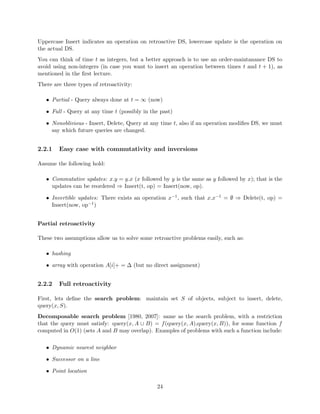
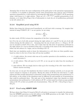
![Claim 1. Full Retroactivity for decomposable search problems (with commutativity and inversions)
can be done in O(lgm) factor overhead both in time and space (where m is the number of operations)
using segment tree [1980, Bentley and Saxe [19]]
Figure 2.1: Segment Tree
We want to build a balanced search tree on time (leaves represent time). Every element lives
in the data structure on the interval of time, corresponding to its insertion and deletion. Each
element appears in lg n nodes.
To query on this tree at time t, we want to know what operations have been done on this tree from
the beginning of time to t. Because the query is decomposable, we can look at lg n dierent nodes
and combine the results (using the function f).
2.2.3 General case of full retroactivity
Roll back method:
write down a (linear) chain of operations and queries
change r time units in the past with factor O(r) overhead.
That's the best we can do in general.
25](https://image.slidesharecdn.com/datastructures-140901161631-phpapp02/85/Data-structures-79-320.jpg)
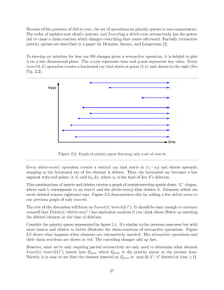
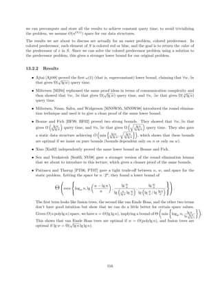
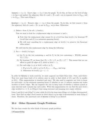
![Because of the presence of delete-min, the set of operations on priority queues is non-commutative.
The order of updates now clearly matters, and Inserting a delete-min retroactively has the poten-tial
to cause a chain reaction which changes everything that comes afterward. Partially retroactive
priority queues are described in a paper by Demaine, Iacono, and Langerman [2].
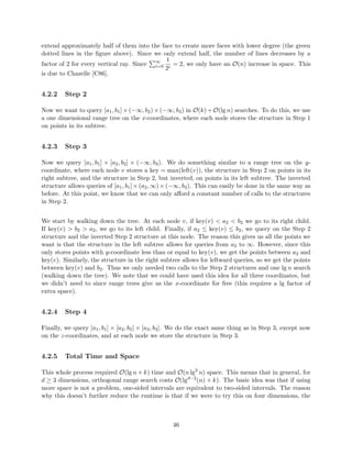
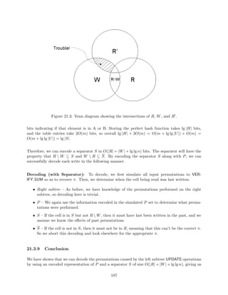
To develop an intuition for how our DS changes given a retroactive operation, it is helpful to plot
it on a two dimensional plane. The x-axis represents time and y-axis represents key value. Every
insert(t; k) operation creates a horizontal ray that starts at point (t; k) and shoots to the right (See
Fig. 2.2).
Figure 2.2: Graph of priority queue featuring only a set of inserts
Every delete-min() operation creates a vertical ray that starts at (t;1) and shoots upwards,
stopping at the horizontal ray of the element it deletes. Thus, the horizontal ray becomes a line
segment with end points (t; k) and (tk; k), where tk is the time of key k's deletion.
This combinations of inserts and deletes creates a graph of nonintersecting upside down L shapes,
where each L corresponds to an insert and the delete-min() that deletes it. Elements which are
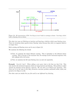
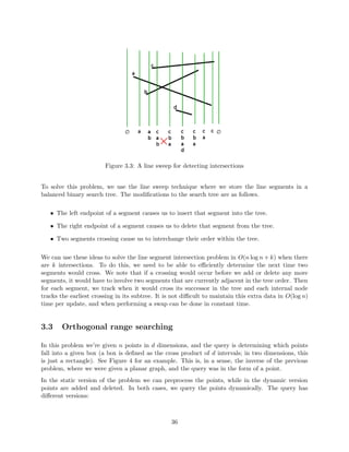
never deleted remain rightward rays. Figure 2.3 demonstrates this by adding a few delete-mins to
our previous graph of only inserts.
The rest of the discussion will focus on Insert(t;insert(k)). It should be easy enough to convince
yourself that Delete(t;delete-min) has equivalent analysis if you think about Delete as inserting
the deleted element at the time of deletion.
Consider the priority queue represented by](https://image.slidesharecdn.com/datastructures-140901161631-phpapp02/85/Data-structures-83-320.jpg)
![nd (incremental connectivity): O(lgm) full
p
mlgm) full. This comes from the fact that any partially retroactive
priority-queue: O(
p
m) factor overhead. It's an OPEN problem
DS can be made fully retroactive with a O(
whether or not we can do better.
successor: This was actually the motivating problem for retroactivity. O(lgm) partial be-cause
it's a search problem. O(lg2m) full because it's also decomposable. However, Giora
and Kaplan gave us a better solution of O(lgm) [16]! This new algorithm uses many data
structures we'll learn about later; including fractional cascading (L3) and vam Emde Boas
(L11).
2.2.7 Nonoblivious Retroactivity
Nonoblivious retroactivity was introduced in a paper by Acar, Blelloch, and Tangwongsan to answer
the question, What about my queries? [17] Usually, when we use a data structure algorithmically
(e.g. priority queue in Dijkstra) the updates we perform depend on the results of the queries.
To solve this problem we can simply add queries to our time line (](https://image.slidesharecdn.com/datastructures-140901161631-phpapp02/85/Data-structures-99-320.jpg)
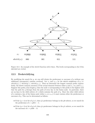
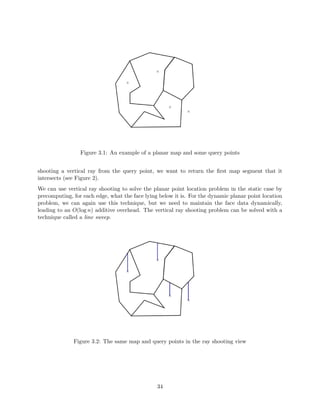
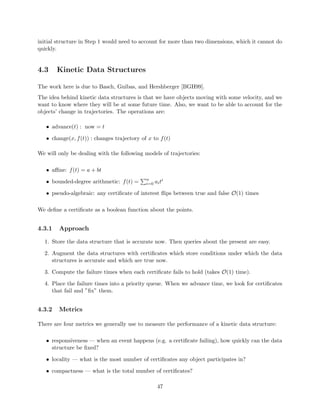
![rst ray that I hit. This
only involves the horizontal segments which are being inserted and deleting. This problem is called
upward ray shooting among dynamic segments. We can solve it in O(lgm) per operation. This
turns out to be the same as the fully retroactive successor problem mentioned earlier which was
proved to be O(lgm) in [16].
The other cases are similar but you also need to use rightward ray shooting.
32](https://image.slidesharecdn.com/datastructures-140901161631-phpapp02/85/Data-structures-111-320.jpg)
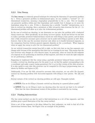
![nd the update corresponding to the
x-coordinate and make a query (using persistence) for (x; y) in that version of the data structure.
It is also useful to note that this structure can be computed in O(n log n) preprocessing time, as
shown by Dobkin and Lipton in [27].
Additionally, if we use the fully retroactive successor data structure, we can solve the dynamic
vertical ray shooting problem with horizontal segments with O(log n) time queries. See [23] and
[29].
Several variants of the vertical ray shooting problem are still open. Examples include:
OPEN: Can we do O(log n) dynamic vertical ray shooting in a general planar graph?
OPEN: Can we do O(log n) static ray shooting when the rays do not have to be vertical?
Note that the three dimensional version of this problem is motivated by ray tracing.
3.2.3 Finding Intersections
The line sweep method can also be used to](https://image.slidesharecdn.com/datastructures-140901161631-phpapp02/85/Data-structures-121-320.jpg)

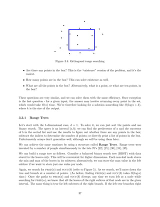
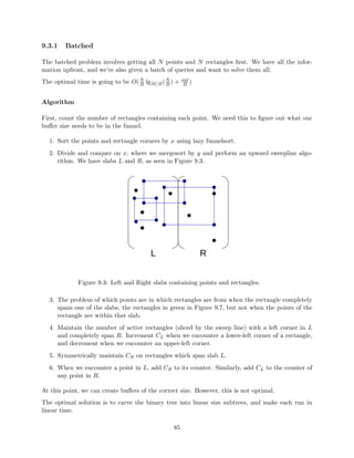
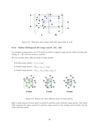
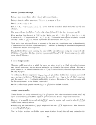
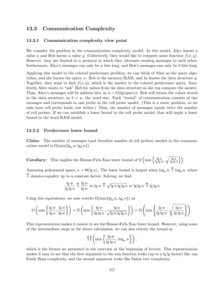
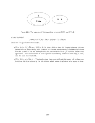
![Figure 3.4: Orthogonal range searching
Are there any points in the box? This is the existence version of the problem, and it's the
easiest.
How many points are in the box? This can solve existence as well.
What are all the points in the box? Alternatively, what is a point, or what are ten points, in
the box?
These questions are very similar, and we can solve them with the same eciency. Once exception
is the last question - for a given input, the answer may involve returning every point in the set,
which would take O(n) time. We're therefore looking for a solution something like O(log n + k),
where k is the size of the output.
3.3.1 Range Trees
Let's start with the 1-dimensional case, d = 1. To solve it, we can just sort the points and use
binary search. The query is an interval [a; b]; we can](https://image.slidesharecdn.com/datastructures-140901161631-phpapp02/85/Data-structures-128-320.jpg)
![gure out whether there are any points in the box;
subtract the indices to determine the number of points; or directly print a list of points in the box.
Unfortunately arrays don't generalize well, although we will be using them later.
We can achieve the same runtimes by using a structure called Range Trees. Range trees were
invented by a number of people simultaneously in the late 70's [22], [21], [30], [31], [35].
We can build a range tree as follows. Consider a balanced binary search tree (BBST) with data
stored in the leaves only. This will be convenient for higher dimensions. Each non-leaf node stores
the min and max of the leaves in its subtrees; alternatively, we can store the max value in the left
subtree if we want to store just one value per node.
Again, we search for pred(a) and succ(b) (refer to Figure 5). As we search, we'll move down the
tree and branch at a number of points. (As before,](https://image.slidesharecdn.com/datastructures-140901161631-phpapp02/85/Data-structures-130-320.jpg)
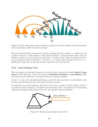
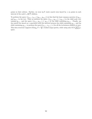
![Figure 3.7: Each of the nodes at the x level have a pointer to all of the children of that node sorted
in the y dimension, which is denoted in orange.
We can extend this idea to d dimensions, storing a y subtree for each x subtree, a z subtree for each
y subtree, and so on. This results in a query time of O(logd n). Each dimension adds a factor of
O(log n) in space; we can store the tree in O(n logd1 n) space in total. If the set of points is static,
we can preprocess them in O(n logd1) time for d 1; sorting takes O(n log n) time for d = 1.
Building the range trees in this time bound is nontrivial, but it can be done.
3.3.2 Layered Range Trees
We can improve on this data structure by a factor of log n using an idea called layered range
trees (See [28], [36], [34]). This is also known as fractional cascading, or cross linking, which
we'll cover in more detail later. The general idea is to reuse our searches.
In the 2 d case, we're repeatedly performing a search for the same subset of y-coordinates, such
as when we search both 2 and
2 for points between a2 and b2.
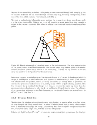
To avoid this, we do the following. Instead of a tree, store an array of all the points, sorted by
y-coordinate (refer to Figure 8). As before, have each node in the x tree point to a corresponding
subarray consisting of those points in the tree, also sorted by their y-coordinate.
Figure 3.8: Storing arrays instead of range trees
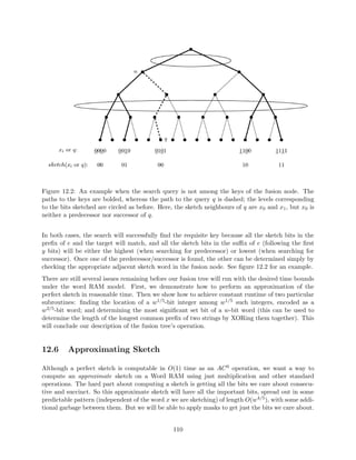
39](https://image.slidesharecdn.com/datastructures-140901161631-phpapp02/85/Data-structures-144-320.jpg)
![dynamic for free using weight balanced trees.
3.3.4 Weight Balanced Trees
There are dierent kinds of weight balanced trees; we'll look at the oldest and simplest version,
BB[] trees [33]. We've seen examples of height-balanced trees: AVL trees, where the left and
right subtrees have heights within an additive constant of each other, and Red-Black trees, where
the heights of the subtrees are within a multiplicative factor of each other.
In a weight balanced tree, we want to keep the size of the left subtree and the right subtree roughly
the same. Formally, for each node v we want
size(left(v)) size(v)
size(right(v)) size(v)
We haven't de](https://image.slidesharecdn.com/datastructures-140901161631-phpapp02/85/Data-structures-148-320.jpg)
![nition. We also haven't selected . If = 1
2 , we have a
problem: the tree must be perfectly balanced at all times. Taking a small , however, (say, = 1
10 ),
works well. Weight balancing is a stronger property than height balancing: a weight balanced tree
will have height at most log1= n.
We can apply these trees to our layered range tree. [31][34] Updates on a weight balanced tree can
be done very quickly. Usually, when we add or delete a node, it will only aect the nodes nearby.
Occasionally, it will unbalance a large part of the tree; in this case, we can destroy that part of the
tree and rebuild it. When we do so, we can rebuild it as a perfectly balanced tree.
Our data structure only has pointers in one direction - each parent points to its children nodes, but
children don't point to their parents, or up the tree in general. As a result, we're free to rebuild
an entire subtree whenever it's unbalanced. And once we rebuild a subtree, we can make at least
(k) insertions or deletions before it becomes unbalanced again, where k is the size of the subtree.
When we do need to rebuild a subtree, we can charge the process of rebuilding to the (k) updates
we've made. Since each node we add can potentially unbalance every subtree it's a part of (a total
of log(n) trees), we can update the tree in log(n) amortized time (assuming that a tree can be
rebuilt in (k) time, which is easy).
So, for layered range trees, we have O(logd n) amortized update, and we still have a O(logd1 n)
query.
3.3.5 Further results
For static
orthogonal range searching, we can achieve a O(logd1 n) query for d 1 using less
space: O
n
logd1(n)
log log n
!
[24]. This is optimal in some models.
We can also achieve a O(logd2 n) query for d 2 using O(n logd(n)) space [25], [26]. A more recent
result uses O(n logd+1(n)) space [20]. This is conjectured to be an optimal result for queries.
There are also non-orthogonal versions of this problem - we can query with triangles or general
simplices, as well as boxes where one or more intervals start or end at in](https://image.slidesharecdn.com/datastructures-140901161631-phpapp02/85/Data-structures-150-320.jpg)
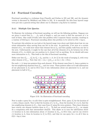
![3.4 Fractional Cascading
Fractional cascading is a technique from Chazelle and Guibas in [25] and [26], and the dynamic
version is discussed by Mehlhorn and Naher in [32]. It is essentially the idea from layered range
trees put into a general setting that allows one to eliminate a log factor in runtime.
3.4.1 Multiple List Queries
To illustrate the technique of fractional cascading, we will use the following problem. Suppose you
are given k sorted lists L1; : : : ;Lk each of length n, and you want to](https://image.slidesharecdn.com/datastructures-140901161631-phpapp02/85/Data-structures-152-320.jpg)

![rst note that we can replace every other element with
of the elements, distributed uniformly, for any small . In this case, we used = 1
2 . However, by
using smaller , we can do fractional cascading on any graph, rather than just the single path that
we had here. To do this, we just (modulo some details) cascade of the set from each vertex along
each of its outgoing edges. When we do this, cycles may cause a vertex to cascade into itself, but
if we choose small enough, we can ensure that the sizes of the sets stays linearly bounded.
In general, fractional cascading allows us to do the following. Given a graph where
Each vertex contains a set of elements
Each edge is labeled with a range [a; b]
The graph has locally bounded in-degree, meaning for each x 2 R, the number of incoming
edges to a vertex whose range contains x is bounded by a constant.
We can support a search query that](https://image.slidesharecdn.com/datastructures-140901161631-phpapp02/85/Data-structures-159-320.jpg)
![ed point in time (advance); (iii) return
information about the state of the objects in the current time. Examples we will go over are kinetic
predecessor/successor and kinetic heaps.
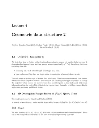
4.2 3D Orthogonal Range Search in O(lg n) Query Time
The work here is due to Chazell and Guibas [CG86].
In general we want to query on the section of our points in space de](https://image.slidesharecdn.com/datastructures-140901161631-phpapp02/85/Data-structures-163-320.jpg)
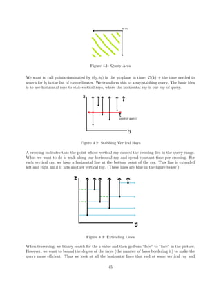
![ned by: [a1; b1][a2; b2][a3; b3].
4.2.1 Step 1
We want to query (1; b2) (1; b3), which we call the restricted two dimensional case. There
are no left endpoints in our query, so the area we're querying basically looks like:
44](https://image.slidesharecdn.com/datastructures-140901161631-phpapp02/85/Data-structures-164-320.jpg)
![gure above). Since we only extend half, the number of lines decreases by a
Pfactor of 2 for every vertical ray. Since
1
i=0
1
2i = 2, we only have an O(n) increase in space. This
is due to Chazelle [C86].
4.2.2 Step 2
Now we want to query [a1; b1](1; b2)(1; b3) in O(k)+O(lg n) searches. To do this, we use
a one dimensional range tree on the x-coordinates, where each node stores the structure in Step 1
on points in its subtree.
4.2.3 Step 3
Now we query [a1; b1] [a2; b2] (1; b3). We do something similar to a range tree on the y-
coordinate, where each node v stores a key = max(left(v)), the structure in Step 2 on points in its
right subtree, and the structure in Step 2, but inverted, on points in its left subtree. The inverted
structure allows queries of [a1; b1](a2;1)(1; b3). This can easily be done in the same way as
before. At this point, we know that we can only aord a constant number of calls to the structures
in Step 2.
We start by walking down the tree. At each node v, if key(v) a2 b2 we go to its right child.
If key(v) b2 a2, we go to its left child. Finally, if a2 key(v) b2, we query on the Step 2
structure and the inverted Step 2 structure at this node. The reason this gives us all the points we
want is that the structure in the left subtree allows for queries from a2 to 1. However, since this
only stores points with y-coordinate less than or equal to key(v), we get the points between a2 and
key(v). Similarly, the structure in the right subtree allows for leftward queries, so we get the points
between key(v) and b2. Thus we only needed two calls to the Step 2 structures and one lg n search
(walking down the tree). We note that we could have used this idea for all three coordinates, but
we didn't need to since range trees give us the x-coordinate for free (this requires a lg factor of
extra space).
4.2.4 Step 4
Finally, we query [a1; b1] [a2; b2] [a3; b3]. We do the exact same thing as in Step 3, except now
on the z-coordinates, and at each node we store the structure in Step 3.
4.2.5 Total Time and Space
This whole process required O(lg n+k) time and O(n lg3 n) space. This means that in general, for
d 3 dimensions, orthogonal range search costs O(lgd2(n) + k). The basic idea was that if using
more space is not a problem, one-sided intervals are equivalent to two-sided intervals. The reason
why this doesn't further reduce the runtime is that if we were to try this on four dimensions, the
46](https://image.slidesharecdn.com/datastructures-140901161631-phpapp02/85/Data-structures-168-320.jpg)
![initial structure in Step 1 would need to account for more than two dimensions, which it cannot do
quickly.
4.3 Kinetic Data Structures
The work here is due to Basch, Guibas, and Hershberger [BGH99].
The idea behind kinetic data structures is that we have objects moving with some velocity, and we
want to know where they will be at some future time. Also, we want to be able to account for the
objects' change in trajectories. The operations are:
advance(t) : now = t
change(x; f(t)) : changes trajectory of x to f(t)
We will only be dealing with the following models of trajectories:
ane: f(t) = a + bt
bounded-degree arithmetic: f(t) =
Pn
i=0 aiti
pseudo-algebraic: any certi](https://image.slidesharecdn.com/datastructures-140901161631-phpapp02/85/Data-structures-169-320.jpg)
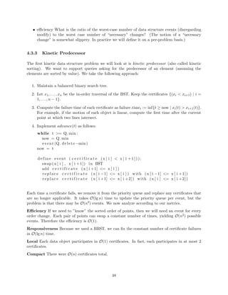
![rst time after the current
point at which two lines intersect.
4. Implement advance(t) as follows:
while t = Q.min :
now = Q.min
event (Q. de l e t emin )
now = t
d e f i n e event ( c e r t i f i c a t e ( x [ i ] x [ i +1 ] ) ) :
swap ( x [ i ] , x [ i +1]) in BST
add c e r t i f i c a t e ( x [ i +1] = x [ i ] )
r e p l a c e c e r t i f i c a t e ( x [ i 1] = x [ i ] ) with ( x [ i 1] = x [ i +1])
r e p l a c e c e r t i f i c a t e ( x [ i +1] = x [ i +2]) with ( x [ i ] = x [ i +2])
Each time a certi](https://image.slidesharecdn.com/datastructures-140901161631-phpapp02/85/Data-structures-186-320.jpg)
![4.3.4 Kinetic Heap
The work here is due to de Fonseca and de Figueiredo [FF03]
We next consider the kinetic heap problem. For this problem, the data structure operation we
want to implement is findmin. We do this by maintaining a heap (for now, just a regular heap, no
need to worry about Fibonacci heaps). Our certi](https://image.slidesharecdn.com/datastructures-140901161631-phpapp02/85/Data-structures-194-320.jpg)