This dissertation examines the behavior of shells supported by elastic foundations. It begins with a critical analysis of existing literature on thin structures like plates, membranes, and shells. It then extends the capstan equation to noncircular geometries for membranes on rigid foundations with friction. Next, it develops a mathematical theory to model shells bonded to elastic foundations, proving existence and uniqueness of solutions. Finally, it introduces a constraint to model shells on elastic foundations with friction, again proving well-posedness. Applications include stretchable electronics and modeling skin abrasion, which is analyzed through numerical simulations validated by experiments.


![Acknowledgments
I thank Dr Nick Ovenden (UCL) for his supervision, University College London for partly funding
this project, The Sidney Perry Foundation [grant number 89], S. C. Witting Trust, Ms Helen Hig-
gins (UCL) for securing funding for the last year of the project, Prof Alan M. Cottenden (UCL),
Mr Clifford Ruff (UCLH) and Dr Sabrina Falloon (UCL) for their assistance with the experiments,
and all the subjects for volunteering for the experiments. I also thank Dr Raul Sanchez Galan
(UCL), Dr Andres A. Leon Baldelli (University of Oxford), Dr Christoph Ortner (University of War-
wick), Prof Dmitri Vassiliev (UCL) and Prof Alan Sokal (UCL) for providing the essential research
material, metalib-c.lib.ucl.ac.uk, scholar.google.co.uk and bookzz.org for making the necessary re-
search material available, and Dr Robert Bowles (UCL), Prof Valery Smyshlyaev (UCL), Dr Edmund
W. Judge (University of Kent), Sir John M. Ball (University of Oxford), Mr Phillip Harvey and Ms
Camille London-Miyo for their assistance.
This work was supported by The Dunhill Medical Trust [grant number R204/0511].
I thank my mother Deepika, my brother Tharinda and my father Chithrasena Guruge for their sup-
port.
Supervisors
Dr Nick Ovenden (UCL) and Prof Alan M. Cottenden (UCL).
Examiners
Dr Christian G. B¨ohmer (UCL) and Dr Evgeniya Nolde (Brunel University).
iv](https://image.slidesharecdn.com/a24f3df3-5be8-40a0-a0ff-910a71f94372-170108131508/85/PhDKJayawardana-4-320.jpg)
![1 Introduction
In this thesis we study the general behaviour of thin curvilinear static isotropic linearly elastic struc-
tures such as shells and membranes when supported by elastic bodies, and in this context such
underlying bodies are commonly referred to as foundations. The significance of this research is that
there exists no comprehensive mathematical theory to conclusively describe the behaviour of thin
objects supported by elastic foundations. Thus, we attempt, with the best of our ability, to present a
mathematical theory of shells supported by elastic foundations.
In Chapter 1 we introduce the critical definitions, fundamental theorems and most notable appli-
cations relating to the study of both shell and membrane theory, as well as contact conditions
governing elastic bodies, in particular, friction. In Chapter 2 we examine behaviour of membranes
supported by rigid foundations where the contact region is governed by the common friction-law. To
be more precise, we extend the capstan equation to a general geometry. Then, we present explicit
solutions and compare our results against other models, in particular, Coulomb’s law of static fric-
tion [102]. In Chapter 3 we begin the study of shells supported by elastic foundations. Initially, we
assume that the shell is bonded, and we derive the governing equations with the mathematical tech-
niques for linear Koiter’s shell theory that is put forward by Ciarlet [38] and a technique that is used
in the derivation of surface Cauchy-Bourne model [89]. In this way, we treat the overlying shell as a
boundary form of the elastic foundation, which is analogous to the work of Necas et al. [144], and
use the mathematical techniques put forward by Ciarlet [38], and Badiale and Serra [13] to mathe-
matically prove the existence and the uniqueness of solutions for the proposed model. Chapter 3
concludes by conducting numerical experiments: by comparing our bonded shell model against an
existing model presented in the literature [16], but modified for our purposes by incorporating gen-
eral elastic properties and extending it to curvilinear coordinates; by checking the numerical validity
of our bonded shell model against the bonded two-body elastic problem. In Chapter 4 we con-
clude our study on shells by asserting that the contact region is governed by a displacement-based
frictional-law that is analogous to Coulomb’s law of static friction. We treat this displacement-based
frictional-law as a constraint, which is analogous to the work of Kinderlehrer and Stampacchia [107],
and with the mathematical techniques put forward by Evans [63], and Kinderlehrer and Stampac-
chia [107] we mathematically prove the existence and the uniqueness of solutions to the proposed
model, and thus, concluding the mathematical theory of overlying shells on elastic foundations.
Chapter 4 concludes by modifying the model for Coulomb’s law of static friction, which is put for-
ward by Kikuchi and Oden [102], to represent two-body elastic problem with friction in curvilinear
coordinates, and we use this extended model to conduct numerical experiments against our shell
model with friction. The reader must understand that, despite we may use other authors’ work as
comparisons, we never use authors’ exact models. We adapt, extend and modify their work to an
extent that they are not original authors’ work, but they are our original work.
We consider Chapter 3 to be the most crucial and the most significant chapter of this thesis as
it contains the most original and fundamental results. Chapter 3, and to a lesser extent Chapter
1](https://image.slidesharecdn.com/a24f3df3-5be8-40a0-a0ff-910a71f94372-170108131508/85/PhDKJayawardana-7-320.jpg)
![4, does not contain mere models: they are mathematical theories. By that what we mean is that,
regardless if our models correctly describe a real life phenomenon or not, the models are mathe-
matically valid as a unique solution exists with respect to an acceptable set of parameters. However,
the work we present in this thesis is by no means complete, and thus, in Chapter 5 we extensively
describe some remaining open questions and limitations of our work. Also, there we present pos-
sible extensions for future work. In Chapter 6 we extend the ideas that we present in Chapters 2,
4 and 5, and propose mathematical models to study the behaviour of in-vivo skin and fabrics in
presence of friction. With real life experimental data gathered from human subjects and numerical
experiment data from our models we attempt to extract some result that maybe implicated in reduc-
ing skin abrasion due to friction. Finally, we conclude our analysis, and thus, this thesis, in Chapter
7, where all our research findings and their significance are discussed.
The following chapter is a comprehensive introduction to the study of thin objects such as plates,
shells, films and other relating subjects that are included in study of mathematical elasticity and
friction. We begin, in Section 1.1, with a list of notations that we subsequently use in the latter
chapters. Sections 1.2 and 1.3 contain all the necessary mathematical definitions and theorems
that are vital for the rigorous mathematical analysis of the later chapters. Here, we are careful in
the accuracy of our sources and our definitions. For example, the definition of hyperelasticity given
by Kikuchi and Oden [102] (see section 5.1 of Kikuchi and Oden [102]) is ‘hyperelastic means that
there exists a differentiable stored energy function ... representing the strain energy per unit volume
of material, which characterizes the mechanical behavior of the material of which the body is com-
posed’ [102]. Although, this is indeed a property of hyperelasticity, it does not merit as a definition
as hyperelasticity is a fundamental concept in mathematical elasticity. For a more precise defini-
tion of hyperelasticity please consult Ball [17] or Ciarlet [38] (see chapter 7 of Ciarlet [38]). Note
that, if having a differentiable energy functional (with respect to the strain tensor) constitutes as the
material being hyperelastic, then any linear elastic material can be hyperelastic as any linear elas-
tic material also have a differentiable energy functional with respect to the strain tensor. However,
this is not the case as one can find a great example by Morassi and Paroni [139] (see section 2
subsection 7.7 of Morassi and Paroni [139] for the examples of convexity and policonvexity) where
the linear elastic model failed to be physically realistic under a condition, while a hyperelastic model
stayed perfectly physically realistic for the same condition. Also, in Sections 1.2 and 1.3 we only
state the theorems and critical results. However, we correctly document the sources so that the
reader may consult for the proofs and the justifications of the results. If the reader is unfamiliar with
pure mathematics, then Sections 1.2 and 1.3 may seem unmotivated or even superfluous, but the
significance of these results is revealed in the subsequent chapters.
Sections 1.4 and 1.5 are dedicated to the study of thin objects. We demonstrate to the reader the
fundamental ideas behind the study of thin objects, the techniques used in deriving of such models
and most notable results in the literature. Sections 1.6 and 1.7 are dedicated to literature of most
notable and relevant commercial applications relating to this work. These sections also double as
a thorough literature review.
2](https://image.slidesharecdn.com/a24f3df3-5be8-40a0-a0ff-910a71f94372-170108131508/85/PhDKJayawardana-8-320.jpg)
![Finally, Sections 1.8, 1.9, 1.10, 1.11 and 1.12 are dedicated to the critical study of vital publications
that paved the way to our current work. Unfortunately, we reveal some authors’ erroneous work that
were responsible for significantly impeding the progress of this project. The reader must understand
that we are not being iconoclastic, but we are merely being mathematically thorough. We urge the
reader not to take our word, but actually review the given publications one’s self as we gone to
great lengths to be meticulous as possible when documenting the flaws (chapters, page numbers,
equations, etc.). In fact, please consult the footnotes for URLs for the free copies of the publications,
so that the reader can make an informative judgement on the matter.
1.1 Notations and Conventions
In this section we present common notations that we use throughout this thesis, but the strict defi-
nitions of the notations are defined in the subsequent sections. The given definitions stand unless
it is strictly says otherwise.
• n ∈ N where N is the set of natural numbers.
• R is usually reserved for a curvilinear real-line.
• E is usually reserved for a Euclidean real-line.
• α, β, γ, δ ∈ {1, 2} are usually reserved for the curvilinear indices.
• i, j, k, l ∈ {1, 2, 3} are usually reserved for Euclidean indices.
• σ : ω ⊂ R2
→ σ(ω) ⊂ E2
describes the unstrained configuration of the shell.
• ¯X : Ω ⊂ R3
→ ¯X(Ω) ⊂ E3
describes the unstrained configuration of the foundation.
• ∂j =
∂
∂xj
are usually describe the partial derivatives with respect to R3
.
• F[I]αβ = ∂ασk∂βσk
is the covariant first fundamental form tensor induced by σ on R2
.
• gij = ∂i
¯Xk∂j
¯Xk
is the covariant metric tensor induced by ¯X on R3
.
• N =
∂1σ × ∂2σ
||∂1σ × ∂2σ||
is the unit normal to the surface σ(ω).
• F[II]αβ = Nk
∂αβσk is the covariant second fundamental form tensor induced by σ on R2
.
• 0 < −
1
2
F α
[II]α signifies positive mean-curvature.
• 0 ≤ F α
[II]αF γ
[II]γ − F γ
[II]αF α
[II]γ signifies nonnegative Gaussian-curvature, i.e. non-hyperbolic.
• β are the covariant derivatives in R2
.
• ¯j are the covariant derivatives in R3
.
• ∂β
= Fαβ
[I] ∂α .
• ∂j
= gij
∂i .
• h is the thickness of the shell or the membrane.
• H is the thickness of the foundation (special case only).
• E is Young’s modulus of the shell or the membrane.
• ¯E is Young’s modulus of the foundation.
• ν is Poisson’s ratio of the shell or the membrane.
3](https://image.slidesharecdn.com/a24f3df3-5be8-40a0-a0ff-910a71f94372-170108131508/85/PhDKJayawardana-9-320.jpg)
![• ¯ν is Poisson’s ratio of the foundation.
• λ =
E
(1 + ν)(1 − 2ν)
is first Lam´e’s parameter of the shell or the membrane.
• ¯λ =
¯E
(1 + ¯ν)(1 − 2¯ν)
is first Lam´e’s parameter of the foundation.
• µ =
1
2
E
(1 + ν)
is second Lam´e’s parameter of the shell or the membrane.
• ¯µ =
1
2
¯E
(1 + ¯ν)
is second Lam´e’s parameter of the foundation.
• Bαβγδ
= µ
2λ
λ + 2µ
Fαβ
[I] Fγδ
[I] + Fαγ
[I] Fβδ
[I] + Fαδ
[I] Fβγ
[I]
is the isotropic elasticity tensor of the shell
or the membrane.
• Aijkl
= ¯λgij
gkl
+ ¯µ gik
gjl
+ gil
gjk
is the isotropic elasticity tensor of the foundation.
• Λ = 4µ
λ + µ
λ + 2µ
.
• is the mass density with respect to the volume of the shell or the membrane.
• l is the width of the membrane.
• δτ = τmax/τ0 = Tmax/T0 is the tension ratio.
• g = 9.81 is the acceleration due to gravity.
• µF is the capstan coefficient of friction.
• νF is Coulomb’s coefficient of friction.
• a is the horizontal radius of the contact region.
• b is the vertical radius of the contact region.
• βδ = arctan
b
a
is the critical parametric-latitude.
• ε is the regularisation parameter.
• |v| 2 =
i
norm(vi
, 2)
2
1
2
, where norm(·, 2) is Matlab 2-norm of matrix.
• R2
is the coefficient of determination of linear regression.
Furthermore, the reader must note the following:
• We assume Einstein’s summation notation unless it strictly says otherwise;
• In numerical modelling, whenever we say Young’s modulus of the shell, we mean Young’s mod-
ulus of the shell relative to Young’s modulus of the foundation, i.e. δE = E/ ¯E. Furthermore, if
δE 1, then we say the shell has a high stiffness;
• In numerical modelling, whenever we say Poisson’s ratio of the shell, we mean Poisson’s ratio of
the shell relative to Poisson’s ratio of the foundation, i.e. δν = ν/¯ν. Furthermore, if 1 δν <
1
2 ¯ν−1
, where ¯ν > 0, then we say the shell is almost incompressible;
• In numerical modelling, whenever we say the thickness of the shell, we mean the thickness of the
shell relative to the thickness of the foundation, i.e. δh = h/H. Furthermore, if δh 1, then we
say the shell is thin;
4](https://image.slidesharecdn.com/a24f3df3-5be8-40a0-a0ff-910a71f94372-170108131508/85/PhDKJayawardana-10-320.jpg)
![• In numerical modelling, whenever we say the vertical radius of the contact region, we mean the
vertical radius of the contact region relative to the horizontal radius of the contact region, i.e.
δb = b/a;
• When discussing numerical results, whenever we speak of a particular variable, we assume all
other variables are fixed unless it is strictly says otherwise;
• All numerical results assume standard SI units unless it is strictly says otherwise;
• All of our numerical modelling is conducted using Matlab 2015b with format long and all numerical
results are expressed in 3 significant figures: always rounded up.
1.2 Measure, Differential Geometry and Tensor Calculus
In this section we present the most important measure theory, differential geometry, and tensor
calculus definitions and theorems that are required in this thesis. Almost all the results given in this
section can be found in Ciarlet [38, 39]1
, Kay [101] and Lipschutz [124].
Definition 1 (σ-algebra). A collection M(Rn
) of subsets of Rn
is called a σ-algebra if
(i) Ø, Rn
∈ M(Rn
),
(ii) U ∈ M(Rn
) ⇒ {Rn
U} ∈ M(Rn
),
(iii) if {Uk}k∈N ⊂ M(Rn
), then k∈N Uk, k∈N Uk ∈ M(Rn
).
Note that n ∈ N and Ø is the empty set in Rn
.
Lemma 1 (Lebesgue Measure and Lebesgue Measurable Sets). There exists a σ-algebra
M(Rn
) of subsets of Rn
and a mapping meas(·; Rn
) : M(Rn
) → [0, +∞] such that:
(i) Every open subset of Rn
and every closed subsets of Rn
are belong to M(Rn
);
(ii) If B is any ball in Rn
, then meas(B; Rn
) is the n-dimensional volume of B;
(iii) If {Uk}k∈N ⊂ M(Rn
), where all Uk are pairwise disjoint, then meas( k∈N Uk; Rn
) =
k∈N meas(Uk; Rn
);
(iv) If U ⊆ V such that V ∈ M(Rn
) and meas(V ; Rn
) = 0, then U ∈ M(Rn
) and meas(U; Rn
) = 0.
Thus, for any U ∈ M(Rn
) we say U is a Lebesgue measurable set and we say meas(·; Rn
) is
the dimensional Lebesgue measure in Rn
.
Proof. Please consult chapter 6 of Schilling [175].
For an introduction on measure theory please consult chapter 1 of Kolmogorov et al. [111].
Definition 2 (Measurable Function). Let f : Rn
→ R. Then we say f is a measurable
function if f−1
(U) ∈ M(Rn
) for every open set U ⊂ R.
Note that f−1
(·) is the preimage of f(·) in this context.
Definition 3 (Essential Supremum ess−sup(·)). Let f : Rn
→ R be a measurable function.
Then the essential supremum of f is ess−sup(f) = inf{a ∈ R | meas({x ∈ Rn
: f(x) > a}; Rn
) =
0}.
1 http://caos.fs.usb.ve/libros/Mechanics/Elasticity/An%20Introduction%20to%20Differential%20Geometry
%20with%20Applications%20to%20Elasticity%20-%20Ciarlet.pdf
5](https://image.slidesharecdn.com/a24f3df3-5be8-40a0-a0ff-910a71f94372-170108131508/85/PhDKJayawardana-11-320.jpg)
![Definition 4 (Almost Everywhere a.e.). Let f, g : Rn
→ R be a measurable functions. Then
we say f = g a.e. if U
[f − g] d(Rn
) = 0, for all U ∈ M(Rn
) with meas(U; Rn
) > 0.
For an introduction on measurable functions please consult chapter 2 of Spivak [184].
We say the map ¯X ∈ C2
(¯Ω; E3
) is a diffeomorphism that describes the reference configuration of
a Euclidean volume with respect to three-dimensional curvilinear coordinates (x1
, x2
, x3
), where
Ω ⊂ R3
is a three-dimensional bounded domain and E3
is the three-dimensional Euclidean space.
By diffeomorphism we mean an invertible map that maps one differentiable manifold to another
such that both the function and its inverse are sufficiently differentiable. Note that Cn
is a space of
continuous functions that has continuous first n partial derivatives in the underlying domain, where
n ∈ N. Bold symbols signify that we are dealing with vector and tensor fields and each must be
understood in the context of the statement. Also, note that we usually reserve the vector brackets
( · )E for vectors in the Euclidean space and ( · ) for vectors in the curvilinear space. Furthermore,
the over-bar in the domain Ω implies the closure of the domain.
The covariant metric tensor of ¯X with respect to curvilinear coordinates is defined as
gij = ∂i
¯Xk∂j
¯Xk
, ∀ i, j ∈ {1, 2, 3} .
Note that ∂j is the partial derivative with respect to the coordinate xj
, and we assume Einstein’s
summation notation. Furthermore, gikgkj
= δj
i , ∀ i, j ∈ {1, 2, 3} where δj
i is the Kronecker delta, and
∂j
= gji
∂i. Einstein’s summation notation is assumed herein unless it is strictly stays otherwise.
Also, we regard the indices i, j, k, l ∈ {1, 2, 3}.
Here the metric tensor is a symmetric positive-definite C1
(¯Ω; R9
) function. By positive definite we
mean that there exists a positive constant C that depends on ¯Ω and ¯X such that Cδijvi
vj
≤ gijvi
vj
,
∀ v ∈ R3
(see section 6.1.1 of Evans [63]). The existence of such a constant can be guar-
anteed as all the three eigenvalues of g are positive in ¯Ω by construction, and thus, let C =
inf(x1,x2,x3)∈¯Ω{λ1, λ2, λ3} where λj are the eigenvalues of g. Also, as g ∈ C1
(¯Ω; R9
), there ex-
ists a finite positive constant M such that M = ess−sup(det(g)).
We say ¯ is the covariant derivative operator in the curvilinear space. For any v ∈ C1
(¯Ω; R3
) we
define its covariant derivative as
¯jvk
= ∂jvk
+ ¯Γk
ijvi
,
where
¯Γk
ij =
1
2
gkl
(−∂lgij + ∂igjl + ∂jgli)
are Christoffel symbols of the second kind. Furthermore, ¯jxi
= δi
j, ∀ i, j ∈ {1, 2, 3}, by definition.
Note that here Christoffel symbols are C0
(¯Ω) functions with symmetry in their lower indices.
6](https://image.slidesharecdn.com/a24f3df3-5be8-40a0-a0ff-910a71f94372-170108131508/85/PhDKJayawardana-12-320.jpg)
![We say ¯∆ is the vector Laplacian operator in the curvilinear space. For any v ∈ C2
(¯Ω; R3
) we define
its vector Laplacian as
¯∆vj
=
1
√
g
∂i
√
g gik ¯kvj
,
where g = det(g) (see page 3 of Moon and Spencer [138]).
We further restrict the map ¯X by asserting that ¯X|x3=0 describes a bounded portion of its boundary,
i.e. given that ∂Ω is the boundary of the domain, there exists a plane ω ⊂ ∂Ω with meas(ω; R2
) > 0
such that x3
= 0 in ω.
We say the map σ ∈ C3
(¯ω; E3
) is an injective immersion that describes the reference configura-
tion of an Euclidean surface with respect to two-dimensional curvilinear coordinates (x1
, x2
), where
ω ⊂ R2
is a two-dimensional bounded plane. By immersion we mean a differentiable map between
differentiable manifolds whose derivative is everywhere injective.
The covariant first fundamental form tensor of σ with respect to curvilinear coordinates is defined
as
F[I]αβ = ∂ασi∂βσi
, ∀ α, β ∈ {1, 2} .
Also, we regard the indices α, β, γ, δ ∈ {1, 2}. Furthermore, F[I]αγFγβ
[I] = δβ
α, ∀ α, β ∈ {1, 2}, by
definition.
The covariant second fundamental form tensor of σ with respect to curvilinear coordinates is de-
fined as
F[II]αβ = Ni∂αβσi
, ∀ α, β ∈ {1, 2} ,
where
N =
∂1σ × ∂2σ
||∂1σ × ∂2σ||
is the unit normal to the surface σ, × is the Euclidean cross product and ||·|| is the Euclidean norm.
Here the first fundamental form tensor is a symmetric positive-definite C2
(¯ω; R6
) function. Thus,
there exists a positive constant C that depends on ¯ω and σ such that Cδαβvα
vβ
≤ F[I]αβvα
vβ
,
∀ v ∈ R2
. Also, as F[I] ∈ C2
(¯ω; R6
), there exists a finite positive constant M such that M =
ess−sup(det(F[I])). Also, the second fundamental form tensor is a symmetric C1
(¯ω; R6
) function.
We say is the covariant derivative operator in the curvilinear plane. For any u ∈ C1
(¯ω; R2
) we
define its covariant derivative as
βuγ
= ∂βuγ
+ Γγ
αβuα
,
where
Γγ
αβ =
1
2
Fγδ
[I] (−∂δF[I]αβ + ∂αF[I]βδ + ∂βF[I]δα)
7](https://image.slidesharecdn.com/a24f3df3-5be8-40a0-a0ff-910a71f94372-170108131508/85/PhDKJayawardana-13-320.jpg)
![are Christoffel symbols of the second kind in the curvilinear plane. Furthermore, βxα
= δα
β ,
∀ α, β ∈ {1, 2}. Note that here Christoffel symbols in the curvilinear plane are C1
(¯ω) functions with
symmetry in their lower indices. Furthermore, as Γγ
αβ ∈ C1
(¯ω), there exists a finite positive constant
M such that ess−sup(Γγ
αβ) ≤ M, ∀ α, β, γ ∈ {1, 2}.
We say ∆ is the vector Laplacian operator in the curvilinear plane. For any v ∈ C2
(¯ω; R2
) we define
its vector Laplacian as
∆vβ
=
1
F[I]
∂α F[I] Fαγ
[I] γvβ
,
where F[I] = det(F[I]) (see page 3 of Moon and Spencer [138]).
Lemma 2. Let ω ⊂ R2
be a plane and let σ ∈ C3
(¯ω; E3
) be an injective immersion. Then there
exists an ε > 0 such that the mapping Θ : ¯ω × [−ε, ε] → E3
defined by
Θ = σ + x3
N
is a C2
(¯ω × [−ε, ε]; E3
)-diffeomorphism with det(∂1Θ, ∂2Θ, ∂3Θ) > 0, ∀ (x1
, x2
, x3
) ∈ ¯ω × [−ε, ε].
Proof. See the proof of theorem 4.1-1 of Ciarlet [39].
Note that × is the Cartesian product in this context.
Proposition 1. Given that (x1
, x2
, x3
) ∈ {ω × (−ε, 0]}, for an ε > 0, the metric tensor, and the
first and the second fundamental forms share the relation
gαβ = F[I]αβ − 2x3
F[II]αβ + x3 2
F[II]αγF γ
[II]β ,
g3β = 0 ,
g33 = 1 .
Proof. A trivial tensor calculus result that follows directly from the definition of ¯X and
lemma 2.
Proposition 2. For a vector v ∈ C1
(¯ω; R3
) the covariant derivative in the curvilinear space
restricted to the plane ω is
¯βvγ
= βvγ
− F γ
[II]β v3
,
¯βv3
= ∂βv3
+ F[II]αβvα
.
Proof. Note that F[II]αβ = ¯Γαβ3|ω = −¯Γ3αβ|ω = −¯Γβ3α|ω and the result follows directly from the
definition of ¯ and lemma 2.
Proposition 3.
αF[II]βγ = βF[II]γα .
Proof. See the proof of theorem 2.5-1 of Ciarlet [38].
Lemma 3 (Gauss’ Theorema Egregium). The Gauss curvature is uniquely determined by
the first fundamental form and is, therefore, preserved by isometries.
8](https://image.slidesharecdn.com/a24f3df3-5be8-40a0-a0ff-910a71f94372-170108131508/85/PhDKJayawardana-14-320.jpg)
![Proof. See the proof of theorem 10.2.1 of Pressley [159].
By isometry we mean a distance-preserving injective map between metric spaces.
Lemma 4 (Fubini’s theorem). Let X, Y ⊂ R be closed intervals and f : X × Y → R. If f is
measurable, then
Y X
f(x, y) dX dY =
X Y
f(x, y) dY dX .
Proof. See the proof of theorem 3-10 of Spivak [184].
Proposition 4. As g ∈ C2
(¯Ω; R9
) is positive definite, there exists a positive constant C that
depends on ¯Ω and ¯X such that
C ≤
Ω
dΩ .
Proof. As g is positive definite, there exists a positive constant c such that c ≤ det(g),
∀ (x1
, x2
, x3
) ∈ ¯Ω. Thus, we get Ω
dΩ = Ω
det(g)
1
2 dx1
dx2
dx3
≥ c Ω
dx1
dx2
dx3
= C. Note that
Ω is a bounded domain in R3
.
Proposition 5. As F[I] ∈ C2
(¯ω; R6
) is positive definite, there exists a positive constant C that
depends on ¯ω and σ such that
C ≤
ω
dω .
Proof. As F[I] is positive definite, there exists a positive constant c such that c ≤ det(F[I]),
∀ (x1
, x2
) ∈ ¯ω. Thus, we get ω
dω = ω
det(F[I])
1
2 dx1
dx2
≥ c ω
dx1
dx2
= C. Note that ω is a
bounded domain in R2
.
Lemma 5 (Positive Definiteness of the Elasticity Tensor). Let ¯E > 0 and −1 < ¯ν < 1
2 . Then
there exists a positive constant C that depends on ¯Ω, ¯X, ¯E and ¯ν such that
Cδik
δjl
MijMkl ≤
¯ν ¯E
(1 + ¯ν)(1 − 2¯ν)
gij
gkl
+
1
2
¯E
(1 + ¯ν)
gik
gjl
+ gil
gjk
MijMkl , ∀ M ∈ S3 .
Proof. See the proof of theorem 3.9-1 of Ciarlet [39].
Note that Sn is the space of n × n real symmetric matrices.
Lemma 6 (Positive Definiteness of the Elasticity Tensor on a General Surface). Let E > 0
and −1 < ν < 1
2 . Then there exists a positive constant C that depends on ¯ω, σ, E and ν such
that
Cδαγ
δβδ
MαβMγδ ≤
1
2
E
(1 + ν)
2ν
(1 − ν)
Fαβ
[I] Fγδ
[I] + Fαγ
[I] Fβδ
[I] + Fαδ
[I] Fβγ
[I] MαβMγδ , ∀ M ∈ S2 .
Proof. See the proof of theorem 4.4-1 of Ciarlet [39].
Lemma 7 (Critical Angle of Deflection of a Semi-Ellipse). Consider the set Semi−Ellipse =
{(a sin(θ), b cos(θ))E | a, b ∈ R>0, θ ∈ [−1
2 π, 1
2 π]}. Let δ be the acute angle that the radial vec-
tor (a sin(θ), b cos(θ))E makes with the unit outward normal vector (ϕ(θ))−1
(b sin(θ), a cos(θ))E,
where ϕ(θ) = (b2
sin2
(θ) + a2
cos2
(θ))
1
2 , i.e.
tan(δ) =
(a2
− b2
)
2ab
sin(2θ) .
9](https://image.slidesharecdn.com/a24f3df3-5be8-40a0-a0ff-910a71f94372-170108131508/85/PhDKJayawardana-15-320.jpg)
![Then the critical value of δ over the set Semi−Ellipse is given by
δcrit =
1
2
π − 2 arctan
b
a
.
Proof. Consider theorem 1 from chapter 8 of Kalman [98], which is proved for the set
Ellipse = {(a sin(θ), b cos(θ))E | 0 < b < a < ∞, θ ∈ (−π, π]} and for the angle δ > 0. Now,
notice that critical points occur at θ = ±1
4 π, and thus, use a few elementary trigonometric
identities to obtain the above lemma.
Definition 5 (Parametric Latitude β(·)). Consider the set Semi−Ellipse = {(a sin(θ), b cos(θ))E |
a, b ∈ R>0, θ ∈ [−1
2 π, 1
2 π]}. Then the parametric latitude is define by β(θ) = arctan((b/a) tan(θ)).
See section 5.5 of Osborne [145].
Consider a prism with an elliptical cross-section defined by the map (x1
, a sin(θ), b cos(θ))E, where
|x1
| < ∞ and θ ∈ [−1
2 π, 1
2 π], then we say βδ = arctan(b/a) is the critical parametric-latitude. To
be more precise, βδ is the parametric latitude with respect to the angle δcrit implied by lemma 7,
i.e. βδ = 1
4 π − 1
2 δcrit . Lemma 7 further implies that βδ ∝ b/a and we use this as a measure of the
curvature of the contact region.
1.3 Functional Analysis
In this section we present the most important functional analysis definitions and theorems that are
required in this thesis. Almost all the results given in this section can be found in Ciarlet [38], Evans
[63], Adams and Fournier [3], and Badiale and Serra [13].
Definition 6 (Segment Condition). We say the domain Ω ⊂ Rn
satisfies the segment con-
dition if for every x ∈ ∂Ω there is a neighbourhood Ux and a nonzero vector yx such that, if
z ∈ ¯Ω ∩ Ux, then z + tyx ∈ Ω for some t ∈ (0, 1).
Segment condition implies that, if the domain Ω is not empty, then the boundary must be (n − 1)
dimensional and the domain cannot lie on both sides of any part of the boundary.
Definition 7 (Uniform-C1
Regularity Condition). We say the boundary of the domain Ω ⊂
Rn
satisfies the uniform-C1
(Rn
; Rn−1
) condition, where n ∈ {2, 3}, if there exists a locally
finite open cover {Uj} of boundary ∂Ω, a corresponding sequence {Φj} of transformations
with first-order continuous partial derivatives and with Φj taking Uj into the ball B = {y ∈
Rn
| ||y|| < 1}, and having Ψj = Φ−1
j such that:
(i) For some finite R, every collection R + 1 of the set Uj has empty intersection;
(ii) For some δ > 0, Ωδ ⊂
∞
j=1 Ψj({y ∈ Rn
| ||y|| < 1
2 });
(iii) For each j, Φj(Uj ∩ Ω) = {y ∈ B | yn > 0};
(iv) There exists a finite constant M such that |∂αΦβ
j (x)| ≤ M, ∀ x ∈ Uj and |∂αΨβ
j (y)| ≤ M,
∀ y ∈ B, ∀ α, β ∈ [1, n].
Definition 8 (Lebesgue Space L2
). Let Ω ⊂ Rn
be a domain and let v ∈ R. Then we say
v ∈ L2
(Ω) if there exists a finite positive constant M such that
||v||L2(Ω) =
Ω
|v|2
dΩ
1
2
≤ M .
10](https://image.slidesharecdn.com/a24f3df3-5be8-40a0-a0ff-910a71f94372-170108131508/85/PhDKJayawardana-16-320.jpg)
![Furthermore, the space (L2
(Ω), || · ||L2(Ω)) is a Hilbert space, i.e. a complete normed space
with the notion of an inner product.
By complete we mean that every Cauchy sequence in the space converges with respect to the
specified norm. Note that the product space (L2
(Ω), || · ||L2(Ω)) must be understood in the context
of the statement. For example, if the tensor E ∈ R2
× R2
is also E ∈ L2
(Ω), then we express
the product space as (L2
(Ω), || · ||L2(Ω)) = (L2
(Ω)×L2
(Ω)×L2
(Ω)×L2
(Ω), (|| · ||2
L2(Ω) +|| · ||2
L2(Ω)+
|| · ||2
L2(Ω) +|| · ||2
L2(Ω))
1
2 ), i.e. ||E||L2(Ω) = ( α,β∈{1,2} ||Eαβ||2
L2(Ω))
1
2 ≤ M for a some finite positive
constant M.
Definition 9 (Sobolev Space Hm
). Let Ω ⊂ Rn
be a domain and let u ∈ R. Then we say
u ∈ H1
(Ω) if there exists a finite positive constant M such that
||u||H1(Ω) =
||u||2
L2(Ω) +
n
j=1
||∂ju||2
L2(Ω)
1
2
≤ M ,
where H1
(Ω) = {v ∈ L2
(Ω) | ∂jv ∈ L2
(Ω) , ∀ j ∈ [1, n]}. Also, we say u ∈ H2
(Ω) if there exists
a finite positive constant M such that
||u||H2(Ω) =
||u||2
L2(Ω) +
n
j=1
||∂ju||2
L2(Ω) +
n
i,j=1
||∂iju||2
L2(Ω)
1
2
≤ M ,
where H2
(Ω) = {v ∈ H1
(Ω) | ∂ijv ∈ L2
(Ω) , ∀ i, j ∈ [1, n]}. The space (Hm
(Ω), || · ||Hm(Ω)) is a
Hilbert space.
Note that ∂iv and ∂ijv from above statements are weak derivatives and must be understood in a
sense of distributions (see section 5.2.1 of Evans [63]). Also, note that H0
= L2
by definition.
Proposition 6 (H¨older Inequality). Let u, v ∈ L2
(Ω), then we have the inequity Ω
|uv| dΩ ≤
||u||L2(Ω)||v||L2(Ω). Also, let ess−sup(¯u) < ∞ and Ω
|¯v| dΩ < ∞, then we have the inequality
Ω
|¯u¯v| dΩ ≤ ess−sup(¯u) Ω
|¯v| dΩ.
Proof. A simple extension of Cauchy-Schwarz inequality. See appendix B.2 of Evans [63].
Proposition 7 (Minkowski Inequality). Let u, v ∈ L2
(ω), then we have the inequality ||u +
v||L2(ω) ≤ ||u||L2(ω) + ||v||L2(ω).
Proof. A simple extension of the triangle inequality. See appendix B.2 of Evans [63].
Definition 10 (Support supp). Let Ω ⊂ Rn
and φ : Ω → R, then we say the support of the
function φ is the set supp(φ) = {x ∈ Ω | φ(x) = 0}.
Definition 11 (Space of smooth functions with compact supports C∞
0 ). Let Ω ⊂ Rn
, then the
space of infinitely differentiable functions with compact support in the underlying domain is
the set C∞
0 (Ω) = {φ ∈ C∞
(Ω) | supp(φ) Ω}, where C∞
is the space of infinity differentiable
functions.
Note that X Ω ⊂ Rn
means that X is compact (closed and bounded) in Rn
such that the closure
of X is a proper subset of Ω.
11](https://image.slidesharecdn.com/a24f3df3-5be8-40a0-a0ff-910a71f94372-170108131508/85/PhDKJayawardana-17-320.jpg)
![Definition 12 (Space of test functions D). Let Ω ⊂ Rn
, then the space of test functions is
the set D(Ω) = {φ ∈ C∞
0 (Ω) | Dα
φ ∈ C∞
0 (Ω) , ∀ α ∈ Nn
}, where D is the differential operator
and α is a multi index.
For more on distribution theory please consult chapter 2 of Demidov [53].
Definition 13 (Sobolev Space H1
0 ). Let Ω ⊂ Rn
, then H1
0 (Ω) is the closure of C∞
0 (Ω) with
respect to the norm in H1
(Ω).
Lemma 8 (Fundamental Lemma of J. L. Lions). Let Ω ⊂ Rn
be a domain and v be a distri-
bution on Ω. If v ∈ H−1
(Ω) and ∂jv ∈ H−1
(Ω), ∀ j ∈ [1, n], then v ∈ L2
(Ω), where H−1
(Ω) is the
dual space of H1
0 (Ω).
Proof. See Magenes and Stampacchia [131].
Lemma 9 (Infinitesimal Rigid Displacement Lemma). Let Ω ⊂ R3
be a domain, ¯X ∈ C2
(¯Ω; E3
)
be a diffeomorphism and v ∈ H1
(Ω). If
¯ivj + ¯jvi = 0 , ∀ (x1
, x2
, x3
) ∈ Ω , ∀ i, j ∈ {1, 2, 3} ,
then there exist two constant Euclidean vectors ¯a, ¯b ∈ E3
such that
vi
∂i
¯X = ¯a + ¯b× ¯X , ∀ (x1
, x2
, x3
) ∈ ¯Ω .
In particular, if v|∂Ω0
= 0, for some ∂Ω0 ⊆ ∂Ω with meas(∂Ω0; R2
) > 0, then ¯a = 0 and ¯b = 0.
Proof. See the proof of theorem 1.7-3 of Ciarlet [38].
Lemma 10 (Infinitesimal Rigid Displacement Lemma on a General Surface). Let ω ⊂ R2
be a plane, σ ∈ C3
(¯ω; E3
) be an injective immersion and v ∈ H1
(ω)×H1
(ω)×H2
(ω). If
¯αvβ + ¯βvα = 0 , ∀ (x1
, x2
) ∈ ω , ∀ α, β ∈ {1, 2} ,
¯α
¯βv3
+ ¯β
¯αv3
= 0 , ∀ (x1
, x2
) ∈ ω , ∀ α, β ∈ {1, 2} ,
then there exist two constant Euclidean vectors a, b ∈ E3
such that
vα
∂ασ + v3
N = a + b×σ , ∀ (x1
, x2
) ∈ ¯ω .
In particular, if v|∂ω0
= 0 and nα
∂αv3
|∂ω0
= 0, for some ∂ω0 ⊆ ∂ω with meas(∂ω0; R) > 0, then
a = 0 and b = 0, where n is the unit outward normal to the boundary ∂ω.
Proof. See the proof of theorem 3.6-3 of Ciarlet [38].
By unit we mean nαnα
= F[I]αβnα
nβ
= 1.
Lemma 11 (Boundary Trace Embedding Theorem). Let Ω ⊂ Rn
be a domain with a uniform-
C1
(Rn
; Rn−1
) boundary, where n ∈ {2, 3}, then the embedding H1
(Ω) → L2
(∂Ω) is continuous.
Proof. See the proof of theorem 5.36 of Adams and Fournier [3].
12](https://image.slidesharecdn.com/a24f3df3-5be8-40a0-a0ff-910a71f94372-170108131508/85/PhDKJayawardana-18-320.jpg)
![By continuous we mean that there exists a constant C that depends on Ω and ∂Ω such that
||v||L2(∂Ω) ≤ C||v||H1(Ω). Note that, if Ω is bounded, then there exists a bounded linear operator
Tr : H1
(Ω) → L2
(∂Ω) such that Tr(v) = v|∂Ω for v ∈ H1
(Ω) ∩ C0
(¯Ω), where C0
(¯Ω) is the space of
uniformly continuous functions on Ω (see section 5.5 of Evans [63]). A word of caution: the trace
theorem presented by Evans [63] does not seem to acknowledge the dimensions of the domain
Ω. The reader must be aware that the dimensions of the domain play a significant role in the con-
tinuousness of the trace embedding into the specified Sobolev space. For a more accurate trace
theorem please consult theorem 5.36 of Adams and Fournier [3] or section 2.6.2 of Necas et al.
[144].
Lemma 12 (Trivial Traces). Let ω ⊂ R2
be a domain with a uniform-C1
(R2
; R) boundary,
then v ∈ H1
0 (ω) if and only if v|ω = 0, where v ∈ H1
(ω).
Proof. See the proof theorem 5.37 of Adams and Fournier [3].
Lemma 13 (Rellich-Kondrachov Theorem). Let Ω ⊂ R3
be a bounded domain with a uniform-
C1
(R3
; R2
) boundary, then the embedding H1
(Ω) → L2
(Ω) is compact. Also, let ω ⊂ R2
be a
bounded domain with a uniform-C1
(R2
; R) boundary, then the embeddings H1
(ω) → L2
(ω)
and H2
(ω) → H1
(ω) are compact.
Proof. See the proof of theorem 6.3 of Adams and Fournier [3].
Note that we say that the embedding (X, || · ||X) → (Y, || · ||Y ) is compact if for every bounded
sequence in (X, || · ||X), under the given embedding, has a convergent subsequence in (Y, || ·
||Y ). Note that Rellich-Kondrachov theorem (lemma 13) is proved for domains that satisfy the cone
condition (see definition 4.10 of Adams [3]). As the uniform-C1
boundary implies the cone condition,
lemma 13 holds.
Definition 14 (Coercive). Let (X, || · ||X) be a Banach space. We say the functional J(·) :
X → R is coercive, if ||vk||X → ∞, then J(vk) → ∞, for any sequence {vk}k∈N ⊆ X.
By Banach space we mean a complete normed-space.
Definition 15 (Fr´echet Differentiable). Let (X, || · ||X) be a Banach space and let U ⊆ X be
an open set. Then we say the functional J(·) : U → R is Fr´echet differentiable at u ∈ U if
there exists a unique linear map J (u) ∈ X such that
lim
||v||X →0
J(u + v) − J(u) − J (u)v
||v||X
= 0 ,
where X is the dual space of X.
By linear we mean that J (u)v is linear in v.
Definition 16 (Gˆateaux Differentiable). Let (X, || · ||X) be a Banach space and let U ⊆ X be
an open set. Then we say the functional J(·) : U → R is Gˆateaux differentiable at u ∈ U if
there exists a linear map JG(u) ∈ X such that
lim
t→0
J(u + tv) − J(u) − JG(u)tv
t
= 0 .
13](https://image.slidesharecdn.com/a24f3df3-5be8-40a0-a0ff-910a71f94372-170108131508/85/PhDKJayawardana-19-320.jpg)
![Lemma 14. Let (X, ||·||X) be a Banach space and let J(·) : U → R be a Gˆateaux differentiable
functional in the open set U ⊆ X. If the Gˆateaux differential is continuous at a point u ∈ U,
then the functional is Fr´echet differentiable at the point u, i.e. JG(u) = J (u).
Proof. Simple extension of continuous partial-derivatives imply differentiability. See the
proof of proposition 1.3.8 of Badiale and Serra [13].
Definition 17 (Local Minimum Point). Let (X, || · ||X) be a normed space and let U ⊆ X be
an open set. Then we say v ∈ U is a local minimum point of the functional J(·) : U → R if
J(u) = minv∈U J(v).
Definition 18 (Critical Point). Let (X, || · ||X) be a Banach space and let U ⊂ X be an open
set. Then we say u ∈ U is the critical point of a Fr´echet differentiable functional J(·) : U → R
if J (u) = 0.
Lemma 15. Let (X, ||·||X) be a Banach space and let J(·) : X → R be a Fr´echet differentiable
functional, then any local minimum point is a critical point.
Proof. See remark 1.5.1 of Badiale and Serra [13].
Definition 19 (Convex). Let (X, || · ||X) be a Banach space. Then we say the functional
J(·) : X → R is convex if J(tu + (1 − t)v) ≤ tJ(u) + (1 − t)J(v), ∀ t ∈ [0, 1] and ∀ u, v ∈ X.
Definition 20 (Strictly Convex). Let (X, || · ||X) be a Banach space. Then we say the func-
tional J(·) : X → R is strictly convex if J(tu + (1 − t)v) < tJ(u) + (1 − t)J(v), ∀ t ∈ (0, 1) and
∀ u, v ∈ X where u = v.
Lemma 16. Let (X, || · ||X) be a Banach space. Then the Fr´echet differentiable functional
J(·) : X → R is strictly convex if it satisfies the relation
0 < (J (u) − J (v)) (u − v) , ∀ u, v ∈ X where u = v.
In particular, if J (u) is linear in u, then there exist a positive constant C such that
C||u − v||2
X ≤ (J (u) − J (v)) (u − v) , ∀ u, v ∈ X .
Proof. See the proof of proposition 1.5.10 of Badiale and Serra [13] and apply definition
20.
Lemma 17 (Unique Global Minimum Point). Let (X, || · ||X) be a Banach space and let
J(·) : X → R be a continuous coercive strictly-convex functional. Then J(·) has a unique
global minimum point.
Proof. Combine the proofs of theorems 1.5.6 and 1.5.8 of Badiale and Serra [13].
Lemma 18 (Unique Critical Point). Let (X, ||·||X) be a Banach space and let J(·) : X → R be
a strictly-convex Fr´echet-differentiable functional. Then J(·) has at most one critical point.
Proof. See the proof of theorem 1.5.9 of Badiale and Serra [13].
14](https://image.slidesharecdn.com/a24f3df3-5be8-40a0-a0ff-910a71f94372-170108131508/85/PhDKJayawardana-20-320.jpg)
![Definition 21 (Closed Graph). Let (X, dX) and (Y, dY ) be metric spaces were is dX and dY
are metrics in respective spaces X and Y . Then we say the map ι : (X, dX) → (Y, dY ) is a
closed graph if the set graph(ι) = {(x, ι(x)) | x ∈ X} is a closed subset of the product space
(X, dX) × (Y, dY ).
Lemma 19 (Closed Graph Theorem). Let (X, || · ||X) and (Y, || · ||Y ) be Banach spaces and
let ι : (X, || · ||X) → (Y, || · ||Y ) be a be a linear map. Then ι is continuous if and only if it has
a closed graph.
Proof. See the proof of theorem 7.19 of Sokal [182].
Herein we assert that the set Ω ⊂ R3
is an open bounded connected domain that satisfies the
segment property with a uniform-C1
(R3
; R2
) boundary, and we assert that the set ω ⊂ R2
is an open
bounded connected domain that satisfies the segment property with a uniform-C1
(R2
; R) boundary,
unless it is strictly says otherwise. By connected we mean a set that cannot be represented as the
union of two or more disjoint nonempty open subsets.
1.4 Beams, Plates and Shells
A plate is a structural element with planar dimensions that are large compared to its thickness.
Thus, plate theories are derived from the three-dimensional elastic theory by making suitable as-
sumptions concerning the kinematics of deformation or the state stress through the thickness of the
lamina, thereby reducing three-dimensional elasticity problem into a two-dimensional one. In this
section we only restrict our attention to displacement-based theories. Note that displacement-based
theories such as Kirchhoff–Love plate theory, Mindlin–Reissner plate theory and Euler–Bernoulli
beam theory are originally derived with the use of Newton’s second law of motion and equilibrium
considerations. However, in this work we review them as equations derived by principle of virtual
displacements. For more on principle of virtual displacements please consult section 2.2.2 of Reddy
[163].
For Kirchhoff–Love plate theory [126] the displacement field is defined as
u(x, y, z) = (u1
(x, y) − z∂xu3
(x, y), u2
(x, y) − z∂yu3
(x, y), u3
(x, y))E .
This is a first-order shear-deformation theory and it is only valid for thin plates and for very small
deflections. The theory assumes that the order of the unknown functions are ∂βuα
= O(ε2
) and
∂βu3
= O(ε), and only the leading order terms are used to derive the governing equations. Fur-
thermore, the following fundamental assumptions of classical plate theory (i.e. Kirchhoff–Love as-
sumptions) are assumed, and they are: (i) straight lines normal to the mid-surface remain straight
after deformation, (ii) straight lines normal to the mid-surface remain normal to the mid-surface after
deformation, and (iii) the thickness of the plate does not change during a deformation [163]. Note
that despite the prevalence Kirchhoff–Love assumptions, they are the subject of some scientific dis-
putes [110].
15](https://image.slidesharecdn.com/a24f3df3-5be8-40a0-a0ff-910a71f94372-170108131508/85/PhDKJayawardana-21-320.jpg)
![Given that q(x, y) is a traverse load and one is dealing with an isotropic plate, the governing equa-
tions reduce to the following form,
Eh3
12(1 − ν2)
∆2
Eu3
− q = 0 ,
where ∆E is the two-dimensional Euclidean Laplacian, E and ν are Young’s modulus and Poisson’s
ratio of the plate respectively. Note that the term 1
12 (1 − ν2
)−1
Eh3
is referred to as the bending
stiffness and it signifies the magnitude of the force that is required to bend a plate in the transverse-
direction per unit-volume.
As for the boundary conditions, one requires at least four boundary conditions per given plate theory.
These boundary conditions include clamped, simply supported and free-end, and each condition
varies from one plate-theory to another. To define each boundary condition in more detail is cum-
bersome, and thus, herein they are not reviewed.
For moderately thicker plates Mindlin–Reissner first-order shear-deformation plate theory is utilised.
For Mindlin–Reissner plate theory [137] the displacement field is defined as
u(x, y, z) = (u1
(x, y) − zφ1
(x, y), u2
(x, y) − zφ2
(x, y), u3
(x, y))E ,
where φ(x, y) = (φ1
, φ2
, 0) are defined as the angles that the normal to the mid-surface makes
with the z = 0 axis. The theory assumes the plane-stress condition, i.e. there is a linear variation
of the displacement across the plate thickness, but the plate thickness does not change during
deformation. This theory is valid for thicker plates as it considers the shear deformations through
the thickness of a plate. For this theory the transverse shear strains are represented as constant
through lamina’s thickness. Thus, it follows that the transverse shear-stress is also constant. It is
known from the elementary theory of homogeneous beams (nonlinear Euler-Bernoulli beam theory
[164]) that the transverse shear-stress variation is parabolic through the beam thickness. This
discrepancy between the actual-stress state and the constant-stress state predicted by the first-
order theory is often corrected by the introduction of the shear-correction factor (see chapter 10 of
Reddy[166]). The theory assumes that the order of the unknown functions are uα
= O(ε2
) and
φβ
, ∂βu3
= O(ε), and only the leading order terms are used to derive the governing equations.
Thus, given that q(x, y) is a traverse load and one is dealing with an isotropic plate, the governing
equations take the form
Eh3
12(1 − ν2)
∆E( E · φ) + q = 0 ,
Ehκ
2(1 + ν)
(∆Ew − E · φ) + q = 0 ,
h2
12(1 − ν)
∆E( E × φ) + κ E × φ = 0 ,
where κ is the shear-correction factor, E is the two-dimensional Euclidean differential operator
and · is the Euclidean dot product operator. Furthermore, given that wK
is the vertical displace-
ment function from Kirchhoff–Love plate theory and wM
is the vertical displacement function from
Mindlin-Reissner plate theory, Wang and Alwis [205] show that the vertical displacement functions
16](https://image.slidesharecdn.com/a24f3df3-5be8-40a0-a0ff-910a71f94372-170108131508/85/PhDKJayawardana-22-320.jpg)
![are related by the relation wM
= wK
+ 1
6 (1 − ν)−1
h2
∆EwK
.
For a second-order plate theory with transverse inextendibility the displacement field is defined as
u(x, y, z) = (u1
(x, y) − zφ1
(x, y) − z2
ψ1
(x, y), u2
(x, y) − zφ2
(x, y) − z2
ψ2
(x, y), u3
(x, y))E ,
where ψβ
are the curvatures at the mid-surface of the plate. The second-order shear deformation
theories are rarely used as the theories incorrectly estimate the in-plane displacements of the points
(x, y, z) and (x, y, −z) to be the same, irrespective of the direction of bending [165].
Unlike Kirchhoff–Love plate theory for first-order deformations, there exists no standard third-order
shear deformation theory. One theory proposed is Reddy plate theory [166]. For Reddy plate theory
the displacement field is defined as
u(x, y, z) = (u1
+ zφ1
− cz3
(φ1
+ ∂xu3
), u2
+ zφ2
− cz3
(φ2
+ ∂yu3
), u3
)E,
where c = 4
3 h−2
. As a consequence of the term c, the displacement field accommodates quadratic
variations of the transverse shear-strains, and thus, stress through the thickness, and vanishing of
transverse shear-stress on the top and the bottom of the plate. Thus, Reddy plate theory requires
no shear-correction factors. Just as in Mindlin–Reissner plate theory the order of the unknown
displacement functions are given by ∂βuα
= O(ε2
) and φβ
, ∂βu3
= O(ε). Assuming that q(x, y) is a
traverse load Reddy and Wang [166] provide a set of governing equations with boundary conditions.
However, the format of the governing equations given in authors’ publication is difficult to decipher.
Thus, if one wishes to, an alternative format comparable with the publication can be formulated as
1
c
1
(1 − 2ν)
∂
∂x
17
128
E · φ −
2
65
∆Eu3
+ ∆E
17
128
φ1
−
2
65
∂u3
∂x
= φ1
+
∂u3
∂x
,
1
c
1
(1 − 2ν)
∂
∂y
17
128
E · φ −
2
65
∆Eu3
+ ∆E
17
128
φ2
−
2
65
∂u3
∂u3
= φ2
+
∂u3
∂y
,
Eh
45c
(1 − ν)
(1 + ν)(1 − 2ν)
[4∆E E · φ − ∆2
Eu3
] = −q .
Now, suppose that wK
is the vertical displacement function from Kirchhoff–Love plate theory and
wR
is the vertical displacement function from Reddy plate theory. Reddy and Wang [166] show
that the displacement functions are related by ∆EwR
− λ2
wR
= λ2
[17
84 h2
∆EwK
− wK
], where
λ = 720h−2
(1 − ν). Note that the plate theory that Reddy and Wang[166] put forward is not a
mathematical theory. It is derived purely in terms of mechanical considerations. The authors never
paid any considerations to the existence of solutions or even variational analysis. Thus, given a spe-
cific problem, the plate theory that the authors proposed may not even have a solution. This implies
that what the authors proposed is merely a mathematical model or a mathematical hypothesis. If
the reader is interested in third-order plate models, Reddy’s models in particular, please consult the
sections 10.3 and 10.4 of [163], where reader can find many numerical results for various examples.
Suppose now that one of the degree of freedom is eliminated from the planer coordinates, and
thus, reducing the two-dimensional plate theory problem into a one-dimensional problem. Such
theories are known as beam theories and they provide methods of calculating the load-carrying
17](https://image.slidesharecdn.com/a24f3df3-5be8-40a0-a0ff-910a71f94372-170108131508/85/PhDKJayawardana-23-320.jpg)
![and deflection characteristics of beams. Thus, if one eliminates the y dependency of Kirchhoff–Love
plate theory, then one obtains Euler–Bernoulli beam theory [195] (for zero-Poisson’s ratio), where
governing equations take the form
EI
∂4
u3
∂x4
− q = 0 , (1)
and where I is the second moment of inertia of the beam.
Euler–Bernoulli beam theory is a good approximation for the case of small deflections of a beam
that are subjected to lateral loads. However, if one also takes into account the shear deformation
and the rotational inertia effects, making it suitable for describing the behaviour of thick beams, then
the most acceptable beam theory to use is Timoshenko beam theory [194]. In fact, Euler–Bernoulli
beam theory is a special case of Timoshenko beam theory. Note that the governing equations for
Timoshenko beam theory maybe derived by eliminating the y dependency from Mindlin–Reissner
plate theory.
Despite the fact that Euler-Bernoulli beam theory is valid only for infinitesimal strains and small
rotations, the theory can be extended to problems involving moderately large rotations by the use
of von Karman strains, provided that the strain remains small, which results in nonlinear Euler-
Bernoulli beam theory [113]. However, in nonlinear Euler-Bernoulli beam theory the stress in the
lateral direction is neglected, even though in large bending lateral stresses are considered to be
significant [206]. Considering this and with the use of the fundamental hypotheses in the beam
theory (i.e. the cross section of a beam, which is perpendicular to the centroid locus before bending,
remain in plane and perpendicular to the deformed locus) Gao [71] modifies Timoshenko beam
theory to model large deflections of beams. The author defines the displacement field as (u(x) −
y∂xw(x), w(x))E, where the orders of the unknowns displacements are given as ∂xu = O(ε2
) and
∂xw = O(ε). Neglecting all O(ε5
) terms the author derives the following governing equations,
Eh3
12
∂4
w
∂x4
−
3
2
Eh
∂2
w
∂x2
∂w
∂x
2
+ λ
∂2
w
∂x2
− (1 − ν2
)q = 0 , (2)
∂u
∂x
+
1
2
(1 + ν)
∂w
∂x
2
+
λ
2h(1 + ν)
= 0 ,
where λ is an integral constant that depends on the x-directional external force on the boundary.
A large part of author’s publication is dedicated to proving the existence of solutions to a contact
problem. For this contact problem the author considers a large deformed beam that is supported
by a rigid obstacle, which is prescribed by a strictly concave function. The author shows that in
the elastic buckling analysis of the beam problem, where λ > 0: the contact problem is a nonlinear
unilateral bifurcation problem. Using a variational inequality approach the author shows that there
exist numerical approaches that one can take to solve the contact problem. Furthermore, for the
case q = 0 equation (2) may be treated as a nonlinear eigenvalue problem. For von Karman plates
the author explore this case in an earlier publication [70].
In a further publication Gao [72] develops two dynamical nonlinear beam theories for precise mod-
elling of post-buckling behaviour with finite deformation. The author shows that for both models that
18](https://image.slidesharecdn.com/a24f3df3-5be8-40a0-a0ff-910a71f94372-170108131508/85/PhDKJayawardana-24-320.jpg)
![the deformations in the thickness direction are proportional to ∂xw(x), which becomes significant
when the beam is subjected to large rotations. The author utilises one of the models to study a
frictional contact problem, and for this, unilateral post-buckling, problem an analytical solution is ob-
tained. This publication is based on the finite deformation theory (very large deformations), which
is beyond the scope of this thesis; hence, it is not reviewed in detail herein.
h
R
(a)
(c)
(b)
Figure 1: ‘A beam (a) before bending and (b) after bending; (c) a close-up of the displace-
ment field’ [84], where h is the thickness of the beam and R is the radius of the curvature
of deformation.
Howell et al. [84]2
propose another method for studying the behaviour of large defections of beams.
Without considering any valid methods in the in the field of finite deformation theory or differential
geometry, the authors derive their own version of the nonlinear Euler–Bernoulli beam equation (see
section 4.9 of Howell et al. [84]), where governing equations take the form
EI
d2
θ
ds2
+ N0 cos θ − T0 sin θ = 0 , (3)
where θ(s) and s are respectively the angle and the arc length between the centre-line of the beam
(see figure 1), and T0 and N0 are the forces applied at the boundary which are parallel to the x and
y axis respectively. The authors assume that the centre-line is virtually unchanged, and thus, large
in-plane strains of the centre-line are ignored in the derivation of the equation (3). What the authors
put forward is flawed and it does not depict a representation of the Euler–Bernoulli beam equation,
nonlinear or otherwise. For a comprehensive study of the nonlinear Euler–Bernoulli beam equation
please consult Reddy [164] or Hodges et al. [81].
To examine why equation (3) is flawed: consider the case where one is bending a beam into a shape
with constant radius of curvature R, where R3
I, by applying appropriate boundary forces N0 and
T0. Then equation (3) reduces to EI d2
ds2 (R−1
s)+N0 cos θ−T0 sin θ = 0. As R is a constant, one finds
that N0 cos θ − T0 sin θ = 0, ∀ θ, and thus, N0, T0 = 0. This implies that it takes no force to bend the
beam with a constant radius of deformation, regardless of the magnitude of the deformation, which
2 https://books.google.co.uk/books?isbn=0521671094
19](https://image.slidesharecdn.com/a24f3df3-5be8-40a0-a0ff-910a71f94372-170108131508/85/PhDKJayawardana-25-320.jpg)
![is not physically viable. Now, the reader can see that when the radius of curvature of deformation is
constant, equation (3) is no longer valid. However, those who are familiar with the beam theory may
argue that one cannot bend a beam so that the radius of the deformation is constant without an ex-
ternal forcing. However, if one considers equation 4.9.3 of the publication, then one can re-express
equation (3) as EI d2
ds2 (R−1
s)+N(θ) = 0, where N(θ) is an normal force acting on the beam. Again,
bend the beam in to a constant radius of curvature R by applying a normal force of N(θ) to obtain
EI d2
ds2 (R−1
s)+N(θ) = 0. As the reader can see that authors’ nonlinear beam equation is, again, no
longer valid, regardless of the magnitude of the deformation, i.e. regardless of the limits of θ or the
magnitude of the constant R. In contrast, consider, if one is to bending a beam into a shape with a
constant radius R by a traverse load q(x) below the x-axis with respect linear Euler–Bernoulli beam
equation (1), then one finds that EI(3(u + R)−3
+ 18x2
(u + R)−5
+ 15x4
(u + R)−7
) + q = 0, where
u =
√
R2 −x2 − R and x R. As the reader can see that Euler–Bernoulli equation stays perfectly
valid under such deformations. Can the reader see now why Howell et al.’s [84] beam theory is
flawed?
The flaws of equation (3) have arisen from the derivation of the equation (see section 4.9.1 of How-
ell et al. [84]) as the authors did not consider any valid mathematical techniques in study of the thin
objects subjected to finite strains and mathematical techniques in study of coordinate transforms.
The authors make a fundamental mistake by assuming that an arbitrary coordinate transform is the
same as a deformation of an elastic body. For a model that is similar in nature, also happens to be
flawed, please see Section 1.9, where we further examine in detail why aspects of Howell et al.’s
[84] derivation of their model fails to work. Note that for a comprehensive mathematical study of thin
bodies (plates and shells) subjected to finite strains please consult sections Bs of Ciarlet [37] and
Ciarlet [38].
Over the recent years many important developments in the field of plate theory are made with the
use of (and the mathematical techniques surrounding) Γ-convergence. Γ-convergence is used to
rigorously justify the passage from three-dimensional to two-dimensional theories in elasticity the-
ory. Friesecke et al. [69] show that the energy functional of nonlinear plate theory is a curvature
functional for surfaces that arises from the Γ-limit of the three-dimensional nonlinear elasticity theory
as the thickness of the plate goes to zero. In a separate publication the authors show that the low
energy Γ-limit of the three-dimensional nonlinear elasticity theory gives rise to Foppl-von Karman
theory [67]. In a further publication the authors present a hierarchy of plate models derived from
nonlinear elasticity theory by Γ-convergence [68]. This is achieved by considering the asymptotic
behaviour of minimisers of three-dimensional nonlinear elasticity theories for plates in the limit as
thickness goes to zero. The authors demonstrate that three-dimensional minimisers converge, after
suitable rescaling, to minimisers of a hierarchy of plate models. This implies that different limiting
theories are distinguished by different scaling exponents of the energy as a function of the thick-
ness. Furthermore, the scaling of the energy is, in turn, controlled by the scaling of the applied
forces. Note that unlike classical derivations of plate theories, no ‘priori’ assumptions are made on
the structure of the three-dimensional solutions. The different theories in the hierarchy are distin-
20](https://image.slidesharecdn.com/a24f3df3-5be8-40a0-a0ff-910a71f94372-170108131508/85/PhDKJayawardana-26-320.jpg)
![guished by the relation between the strength of the applied force and the thickness. If the reader
is more interested in the subject, then an introduction to Γ-convergence methods for thin structures
can be found in section 3 of Morassi and Paroni [139].
Mathematical shells are thin objects where the rest configuration exists in some curvilinear plane.
To examine shells further, which we do in this thesis, let us derive linearised Koiter’s shell equations
presented by Ciarlet [38]. Before we proceed any further we inform the reader that the method in
which we derive the equations is not the conventional method of derivation. Here, we derive the
shell equations in a differential geometry fashion so that the reader may get a better understanding
of the governing equations of thin elastic bodies in curvilinear coordinates. A more rigorous method
of deriving the shell equations, in means of asymptotics, is found in Ciarlet [38] which the reader is
urged to consult (for plates please consult Ciarlet [37]).
x3
= ×( , )⊂R3
h
X
(
)
X( ) ⊂E 3
N
_
h
hh
_
x
y
z
x1
x2
Figure 2: The reference configuration of an elastic shell (adapted from Ciarlet [39]).
Let ω ∈ R2
be a connected open bounded domain with a sufficiently smooth boundary ∂ω. Now,
let σ : ω → E3
be a smooth enough injective-immersion. Given that h is sufficiently small, Θ :
ω × (−1
2 h, 1
2 h) → E3
describes a diffeomorphism where Θ = σ(x1
, x2
) + x3
N(x1
, x2
) (see figure
2). Now, consider the energy functional of an isotopic linearly elastic body in curvilinear coordinates
described by the equation
J(v) =
ω×(− 1
2 h, 1
2 h)
1
2
Aijkl
Eij(v)Ekl(v) − fi
vi d(ω × (−
1
2
h,
1
2
h))
−
∂ω×(− 1
2 h, 1
2 h)
τi
0vi d(∂ω × (−
1
2
h,
1
2
h)) , (4)
where v ∈ H1
(ω × (−1
2 h, 1
2 h)) is the displacement field, f ∈ L2
(ω) is an external force density field
and τ0 ∈ L2
(ω) is a traction field. Note that in equation (4) the isotropic elasticity tensor is defined
21](https://image.slidesharecdn.com/a24f3df3-5be8-40a0-a0ff-910a71f94372-170108131508/85/PhDKJayawardana-27-320.jpg)
![first fundamental form tensor and ρ is the change in the second fundamental form tensor.
In light of above analysis, consider the map of the deformed mid-surface
R(u) = σ + σ,αuα
+ Nu3
,
where u ∈ H1
(ω)×H1
(ω)×H2
(ω) is the displacement field with respect to the mid surface. Assert
that
σ,αvα
+ Nv3
+ x3
(N + N,αvα
) = σ,αuα
+ Nu3
+ x3 R,1(u) × R,2(u)
||R,1(u) × R,2(u)||
.
Once the above relation is linearised in u, one finds
vβ
(u) = uβ
− x3 ¯ β
u3 , (9)
v3
(u) = u3
. (10)
As a result of the new values of vj
(u), one can re-express the strain tensor as an explicit function
of x3
. Thus, with the use of equations (9) and (10), one can re-express the nonzero components of
the strain tensor as
Eαβ(u) = αβ(u) − x3
ραβ(u) + O((x3
)2
) , (11)
where
αβ(u) =
1
2
¯αuβ + ¯βuα |ω ,
ραβ(u) =
1
2
¯α
¯βu3
+ ¯β
¯αu3
|ω .
Substituting equations (8) and (11) into equation (4), one obtains
J(u) =
1
2 h
− 1
2 h ω
1
2
Bαγ
βδ Eβ
α(u)Eδ
γ(u) − fi
ui +O(x3
) dωdx3
+O(x3
)
−
1
2 h
− 1
2 h ∂ω
τi
0 ui +O(x3
) d(∂ω)dx3
+O(x3
) .
Ignoring any O(x3
) from both volume and the boundary elements from the above equation, integrat-
ing over the interval [−1
2 h, 1
2 h] to eliminate the x3
dependency and finally ignoring all O(h5
) terms
one obtains the energy functional of a shell,
J(u) =
ω
1
2
Bαβγδ
h αβ(u) γδ(u) +
1
12
h3
ραβ(u)ργδ(u) − hfi
ui dω −
∂ω
hτj
0 uj d(∂ω) ,
where
Bαβγδ
= µ
2λ
λ + 2µ
Fαβ
[I] Fγδ
[I] + Fαγ
[I] Fβδ
[I] + Fαδ
[I] Fβγ
[I]
is the isotropic elasticity tensor of a shell,
αβ(u) =
1
2
(F[I]αγ βuγ
+ F[I]βγ αuγ
) − F[II]αβu3
is the half of the change in first fundamental form tensor, and
ραβ(u) = α βu3
− F[II]αγF γ
[II]β u3
+ F[II]βγ αuγ
+ F[II]αγ βuγ
+ ( αF[II]βγ) uγ
is the change in second fundamental form tensor.
For future reference we define the stress tensor of a shell as ταβ
(u) = Bαβγδ
αβ(u) and the
negative of the moments density tensor of a shell as ηαβ
(u) = Bαβγδ
ραβ(u).
23](https://image.slidesharecdn.com/a24f3df3-5be8-40a0-a0ff-910a71f94372-170108131508/85/PhDKJayawardana-29-320.jpg)
![1.5 Films and Membranes
A membrane is defined as a thin-walled body that can only transmit internal forces tangent to its
deformed shape, and thus, the normal components of the stress tensor of the object may consid-
ered to be zero. The study of such materials is known as membrane theory. Membrane theory
acknowledges two types of membranes: shell and true membranes. Shell-membranes are derived
from suppressing stress couples and transverse shear in the shell equations compared with tan-
gential force resultants. This suppression takes place in force equilibrium equations, force boundary
conditions, energy and moment equilibrium around the normal of the shell. Shell-membranes are
capable of modelling regions of the shell that cannot undergo inextensional bending and they are
considered to support compressive stress without wrinkling until buckling take place [121]. True-
membranes are derived by considering two-dimensional sheets (planar or curved) that are formally
incapable of supporting any stress couples or transverse shears, and by assuming that they can
only sustain tangential force resultants. They cannot sustain compressive stresses and they exhibit
wrinkle fields to compensate for the nonexistence of compressive stresses. True-membranes can
accept lines of angular discontinuity in the deformation pattern on the boundary or within the interior,
while in shell-membranes the angular continuity is preserved. Also, unlike shell-membranes, true-
membranes can sustain large inextensional deformations [26]. True-membranes are often used in
modelling certain biological tissues, inflatables, soap bubbles and even shells subject to immense
pressure and strain.
A grossly oversimplified definition of a true-membrane is a shell that is independent of any trans-
verse effects. Thus, for our use, we eliminate the u3
and the O(h3
) dependencies from linearised
Koiter’s shell equations to obtain the energy functional of a true-membrane,
J(u) = h
ω
1
2
Bαβγδ
αβ(u) γδ(u) − fα
uα dω − h
∂ω
τα
0 uα d(∂ω) , (12)
where αβ(u) = 1
2 ( αuβ + βuα) is the strain tensor of the membrane.
A grossly oversimplified definition of the energy functional of a shell-membrane is, again, de-
fined by equation (12), but with the exception that the strain tensor is now defined as αβ(u) =
1
2 ( ¯αuβ + ¯βuα)|ω. Please consult chapters 4 and 5 of Ciarlet [38] for a comprehensive analysis on
the theory of shell-membranes.
As for films, a grossly oversimplified definition of a film is a membrane whose reference domain is a
subset of the two-dimensional Euclidean plane, i.e. the rest configuration is flat. For our purposes,
we define the energy functional of a film as
J(u) = h
ω
µλ
λ + 2µ
α
α(u) β
β(u) + µ β
α(u) α
β (u) − fα
uα dω − h
∂ω
τα
0 uα d(∂ω) ,
where αβ(u) = 1
2 (∂αuβ + ∂βuα) is the strain tensor of the film, and x1
= x and x2
= y.
If the reader is interested to find out more about this subject please consult chapter 7 of Libai and
Simmonds [121], where the authors present a comprehensive study on the nonlinear membrane
24](https://image.slidesharecdn.com/a24f3df3-5be8-40a0-a0ff-910a71f94372-170108131508/85/PhDKJayawardana-30-320.jpg)
![theory. This publication includes topics such as aximembranes (membranes whose unstrained
shapes are surfaces of revolution), cylindrical membranes (initially cylindrical membranes that are
subject to pressure so that the membranes stretch to become non-cylindrical) and edge effects in a
partially wrinkled aximembranes.
1.6 Capstan Equation and Applications in Cable Drive Systems
The capstan equation, otherwise known as Euler’s equation of tension transmission, is the relation-
ship governing the maximum applied-tension Tmax with respect to the minimum applied-tension T0
of an elastic string wound around a rough cylinder. Thus, the governing equation is given by
Tmax = T0 exp(µF θ) , (13)
where θ is the contact angle and µF is the coefficient of friction. By string we mean a one-
dimensional elastic body, and rough is an engineering term that implies that the contact area exhibits
friction. Note that the coefficient of friction is the physical ratio of the magnitude of the shear force
and the normal force between two contacting bodies. The capstan equation is the most perfect
example of a belt-friction model, which describes behaviour of a belt-like object moving over a rigid
obstacle subjected to friction [162]. In engineering the capstan equation describes a body under
a load equilibrium involving friction between a rope and a wheel like circular object, and thus, it is
widely used to analyse the tension transmission behaviour of cable-like bodies in contact with circu-
lar profiled surfaces, such as in rope rescue systems, marine cable applications, computer storage
devices (electro-optical tracking systems), clutch or brake systems in vehicles, belt-pulley machine
systems and fibre-reinforced composites [97].
One of the largest applications of the capstan equation is in electronic cable drive systems, and
notable devices include printers, photocopiers and tape recorders [19]. The most resent applica-
tions can be found in the field of robotics. Cable drive systems are fundamental in the design and
manufacture of high-speed pick-and-place robots (DeltaBot, BetaBot and DashBot), wearable robot-
assisted rehabilitation-devices (robotic prosthetics), biologically-inspired humanoid-robots (ASIMO
by Honda [185]), and haptic devices. For high-speed pick-and-place robots high-speed, high-
acceleration and low-inertia (ability to rapidly accelerate with minimum force) is required [21]. Wear-
able robot-assisted rehabilitation-devices and biologically-inspired humanoid-robots require to be
light weight, have low inertia, have high stiffness (precise motion control and able to maintain
its rigidity), and have backdrivable transmission with zero backlash [18, 143, 156]. Thus, cable
drive systems are widely used in robot applications because of their low inertia, low backlash,
high stiffness and simplicity. Further great advantage of using cable drive devices, especially in bio-
mechanical robots, is that actuators (motors) do not need to be placed at each joint since the cables
(or tendons) can transmit force from a distance. Also, complex designs can be realised due to the
flexibility of the cables, which justifies the use of cable drive systems in portable robotic prosthetics
devices [99]. Note that backdrivable is an engineering term given to a system where the system
can be physically moved when the motor(s) governing the system is (are) not operational. Backlash
is an engineering term given to the clearance or the lost motion in a mechanism caused by gaps
25](https://image.slidesharecdn.com/a24f3df3-5be8-40a0-a0ff-910a71f94372-170108131508/85/PhDKJayawardana-31-320.jpg)
![between the moving parts. A haptic device is an engineering term given to devices that use tactile
feedback technology to recreate the sense of touch by applying forces, vibrations, or motions to the
user.
Baser and Konukseven [19] present an analytical method developed for predicting the transmission-
error of capstan drives due to cable slippage, as prior to the publication, the literature is devoid of
both a common theory of capstan drive transmission-error, due to slippage, and its experimental
validation. The authors develop a theory of wire capstan drive slippage for haptic device applica-
tions and verify the model in experimental tests. The theory based on the classic capstan equation
which is then extended to include the capstan drive slip error. The authors assume that the bending
stiffness of the cable is negligible and in the contact region, of the cable and the drum, the frictional
relationship is linear. Experiments conducted on a thin rope with a 0.35mm diameter show that the
slip of a capstan drive occurs, and results agree with the theory within 10% difference. The authors
hope that the resulting analytical models provide a tool for the designers to predict the slip of cap-
stan drives and allow the models to be utilised in the control algorithms.
Lu and Fan[130] present an analytical method to predict the transmission-backlash of precise-cable-
drive systems. Authors’ work is significant as transmission-backlash of precise-cable-drive systems
is usually neglected as it is much smaller in magnitude than the backlash from gears, chains and
other drives [29, 91, 189]. However, the existence of transmission backlash affects the precision and
dynamic performance of the drive system, which cannot be neglected in high precision applications.
The backlash also affects both the anti-resonance and resonance frequencies of a system, and the
increase of the backlash magnitude [14, 135, 180]. Thus, the authors argue that it is necessary to
develop both theoretical and experimental methods to predict the backlash transmission. Authors’
analysis shows that as the load and centre distance increase, backlash also increases. Also, as
the coefficient of friction and output drum radius increase, the backlash decreases. Increasing the
preload force decreases the backlash, and the effect cause by decreasing the preload force is ap-
pears to be more significant relative to other parameters. The authors show that their experimental
values fit well with the theoretical curve of transmission backlash. Also, they show experimentally
that the transmission backlash of a precise cable drive is usually several sub-milli-radians and it is
given to be significantly smaller than the backlash in gear, chains and belt drive, which is usually
in tens of milli-radians. The authors hope that the theoretical method presented is to be used for
design guidance and initial performance predictions.
Kang et al. [99] present a design of a passive break for a cable drive system, which is named
by the authors as the capstan brake. Consider the following example of a robotic hand grabbing
an object. As the actuating motor moves the finger, i.e. before the finger reaches the object, the
robotic hand operates within the normal energy efficiency range (a real life example can be found
in Kim et al. [103]). However, once in contact with the object, the motor still needs to apply torque
to maintain in this position. Thus, as a result of backdrivability, energy dissipates even through the
motor is not generating mechanical work [42]. To circumvent this problem Kang et al. [99] design a
26](https://image.slidesharecdn.com/a24f3df3-5be8-40a0-a0ff-910a71f94372-170108131508/85/PhDKJayawardana-32-320.jpg)
![non-backdrivable break with a cylinder (capstan) and two one-way clutches (see figure 3). Previous
methods for non-backdrivable actuators, introduced by others, include worm gear pairs and lead-
screws [32, 122], high reduction ratio transmissions [112, 157], and customised clutches [35, 42].
Figure 3: ‘Design of the brake system’ [87].
Kang et al. [99] state that their device it is capable of delivering enough brake force and its breaking
force can be adjusted by simply changing the number of windings, and thus, making the device
adaptable for various other devices. However, with each additional winding the external force re-
quired to release the cable increases, which results in a lower controllability of the device. The
capstan does not reduce the maximum winding force and mechanical work. Experimental results
show that lower than 2N is required to rotate the capstan. But, more importantly, releasing the cable
is not an issue if the proper external force is present. The maximum brake force is approximately
equal to 55N, which is suitable for a cable (tendon) driven wearable robotic arms [86], which is the
intended application for the device.
Another application of the capstan equation can be found in the field of textiles, where tensioned
fibres, yarns, or fabrics are frequently in contact with cylindrical bodies [95]. Doonmez and Mar-
marali [59] demonstrate the knitability of a yarn before knitting. The authors use a variation of the
capstan equation with multiple regression analysis (analogous to hypothesis 4) and equations that
depend on yarn’s characteristics to predict yarn-needle and yarn-yarn friction values.
Many researchers report that the classical capstan equation does not hold in certain situations as
it neglects bending stiffness. Thus, much research is devoted to incorporate bending stiffness into
the capstan equation [34, 78]. Another limitation of the capstan equation is that it is based on an
over-simplified friction theory, which stems from Amontons’ laws. It is generally accepted in the field
of polymers that the coefficient of friction, between fibres and other contacting surfaces, is not a
27](https://image.slidesharecdn.com/a24f3df3-5be8-40a0-a0ff-910a71f94372-170108131508/85/PhDKJayawardana-33-320.jpg)
![constant as Amontons’ laws imply, but it is a variable that depends on the conditions such as the
minimum applied-tension [97] (analogous to figure 9). Further evidence for this statement can be
found in Martin an Mittelmann [134], where the authors find the coefficient of friction of wool fibres
measured by experiments with the use of the classical capstan equation reduces by as much as
50% with an increase of the minimum applied-tension (analogous to figure 25). One of the attempts
to include bending stiffness is given by Wei and Chen [207], where the authors give a theoretical
model for the capstan equation for nonflexible fibres and yarns. Wei and Chen [207] consider the
radius of the capstan and the yarn, and present two solutions for yarns (and fibres) with linear and
nonlinear behaviours respectively. The authors conclude by saying that the theoretical model can
be used to calculate the actual tension of cables with bending stiffness.
Jung et al. [95] present a mathematical model to incorporate bending stiffness into the capstan
equation. The authors consider an inextensible beam and propose a mathematical model with
an analytical solution. One numerical experiment suggests that the difference in the tension ratio
(the ratio between the maximum and the minimum applied-tensions) between the classical and the
modified results can be up to 71% for a mere 10◦
variation in the angle of inclination. In another
publication, Jung et al. [97] present a capstan equation with bending stiffness and with nonlinear
frictional behaviour. The authors consider a power-law friction model in place of Amontons’ laws
friction, which is adapted from the work of Howell [82, 83]. The authors criticise Howell’s [82, 83]
model, and assert that the coefficient of friction must not vary with the change of the beam radius
and the capstan radius as Howell suggested, which is the basis for Jung et al.’s [97] power law.
They show that using their power-law friction or including the rod bending stiffness can change the
tension ratio. In a further publication the authors present a capstan equation with bending stiff-
ness, nonlinear frictional behaviour and Poisson’s ratio [96]. One of authors’ findings show that
presence of a nonzero Poisson’s ratio tends to increase the tension ratio (analogous to figure 65).
Unfortunately, Jung et al.’s [95, 97] mathematical work appear to be questionable as the authors
assumptions and mathematical techniques are not consistent with nonlinear bending theories in
study of thin objects (plates, beams etc.). A more precise analysis of the large deflection of beams
over rigid obstacles can be found in the work of Gao [71, 72].
Kim et al. [105] present a finite-element solution for the capstan equation, where the authors model
a three-dimensional aluminium-sheet deforming over a rigid cylinder. The friction is calculated by
the friction model put forward by Swift [190]. The simulation shows non-uniform pressure distri-
butions, both in the longitudinal and transverse directions of the contact surface, which include
pressure peaks near the inlet and the outlet regions, and near the strip edges (see figure 4). This
contradicts the results obtain by the simple capstan equation (13) and the work of Saha and Wilson
[172], where one can observe a monotonic increase in pressure from the inlet region to the outlet
region. Given an initial coefficient of friction µF = 0.1 and the contact angle θ = 90◦
, Kim et al.
[105] find the final coefficient of friction is µF = 0.093 and the contact angle is θ = 74◦
. The loss
of contact is clearly due to the bending stiffness of the aluminium-sheet as a portion of the applied
force is expended on overcoming the bending stiffness; however, the reduction in the coefficient of
28](https://image.slidesharecdn.com/a24f3df3-5be8-40a0-a0ff-910a71f94372-170108131508/85/PhDKJayawardana-34-320.jpg)
![z
z
z
x x
x
1
2
3
4
Row
7
.
.
0°
45°
90°
-10
10
30
50
70
90
110
130
150
0 15 30 45 60 75 90
Angle
Pressure(MPa)
Row1 Row2 Row3
Row4 Row5 Row6
Row7
Figure 4: Contact pressure distribution at each row at time = 1.024s, where the contact
angle is in degrees and contact pressure is in megapascals [87].
friction is not a factor of the final contact-angle. The author conclude that further investigation is
needed with various geometries and test conditions.
In a rather older publication, Stuart [187] finds similar results to Kim et al. [105]. Stuart et al. [187]
attempts to incorporate bending stiffness with the capstan equation, where the friction governed by
Amontons’ laws. Among other research findings, the author shows that a reduction in the contact
angle and a variable coefficient of friction throughout the contact profile, which are two of the no-
table results that Kim et al. [105] discover in their finite-element experiments.
Due to the lack of time and resources we cannot verify the validity of the work of the authors
discussed in this section. However, we analyse the mathematical aspects of this subject in great
detail in Chapter 2, where we examine the theory and the behaviour of the capstan equation for
non-cylindrical geometries.
1.7 Applications in Flexible and Stretchable Electronics
In recent years flexible and stretchable electronics become a common technology. Few notable
commercially available devices that use this technology are the LG G Flex phone and the LG
77EG9900 4K Flexible OLed TV. Other than conformal displays, which can be folded or rolled [65],
stretchable electronics have applications in thin film solar cells [33, 50, 117, 147], electronic skins
for robots and humans [203], conformable electronic textiles [27] and complex curvilinear stretch-
able devices for biomedical applications [108]. For such applications the degree of the deformation
of the electronic body can endure, before its basic functions (i.e. conductivity, transparency or light
emission) are adversely affected, is immensely important. However, design and process engineers
who are working on the implementation of flexible electronics often lack confidence due to a lack
of understanding or a lack of input data for reliable modelling tools [125]. Thus, there is a tremen-
dous amount research is conducted in the field of academia (Oxford Centre for Nonlinear Partial
Differential Equations, Lu Research Group the University of Texas at Austin, Flexible Electronics
29](https://image.slidesharecdn.com/a24f3df3-5be8-40a0-a0ff-910a71f94372-170108131508/85/PhDKJayawardana-35-320.jpg)
![Figure 5: ‘Transferred 2cm×2cm silicon nanomembrane on polyimide film’ [213].
and Display Center Arizona State University) as well as in the commercial sector (LG Electronics
[215, 183], Samsung Group [90, 104, 106]).
In a mathematical perspective modelling of such materials follows the following exact procedure. A
thin film (often an inorganic conductor such as copper) is bonded to a thin elastic material, which
in the literature defined as a substrate. In mathematical elasticity language: a film bonded to an
elastic foundation. The problem can now be tackled with just the techniques of solid mechanics.
The research mainly focuses on debonding between the film and the substrate, and the plastic de-
formation of the film due to stretching and the bending of the substrate.
Tensile cracking
and delamination
Neutral axis
(critical)radius
ofcurvature
Compressive buckling
and delamination
Total
strain
Internal
strain
Bending
strain
Neutral axis
z
Figure 6: ‘Summary sketch of damage events and strain state in a flexed substrate coated
on both sides with thin films’ [125].
Figure 6 is a simple visual representation, form Logothetidis [125], of the damage and the state of
strain in an elastic substrate with thin brittle films bonded to both surfaces. Upon bending the body
to some radius of curvature, the film located on the upper surface experiences tensile strain, and
30](https://image.slidesharecdn.com/a24f3df3-5be8-40a0-a0ff-910a71f94372-170108131508/85/PhDKJayawardana-36-320.jpg)
![may fracture and eventually debond. The film located beneath experiences compressive strain and
may also debond, buckle and possibly fracture. The neutral axis is the plane where the strain is
assumed to not change upon pure bending (this assumption is an erroneous for large deflections,
for a comprehensive mathematical study of large deflections of plates please consult section B of
Ciarlet [37]), and the total strain is the sum of the internal strain and the bending strain. The critical
radius of curvature is among the key design parameters for flexible electronics. It is defined as
the radius of curvature at which device failure occurs due to significant mechanical damage or func-
tional failure. For such objects, applications can be found in the transfer-printing of nanomembranes
with polymeric stamps, and annular rubbery gaskets and sealers under uniaxial compression during
service [160].
Logothetidis [125] defines the classification of different branches of stretchable and flexible electron-
ics as: (i) flexible electronics, which comprise films with crit < 2%, which are based on substrate
materials that are thin enough (100mm) to be safely bent to a minimum radius of curvature of 10mm,
but cannot be stretched, (ii) compliant electronics, for which 2% < crit < 10%, which can be flexed
to radius of curvature of few millimetres to allow some in-plane loading and can be used with thicker
substrates, and (iii) stretchable electronics, for which crit > 10%, which can be conformed to a broad
diversity of surfaces with two-dimensional curvatures and small radii below a few millimetres. Note
that crit is the critical strain, where strain exceeding this value results in irreversible mechanical
failure. If the reader is interested more on this subject, especially on the applied mathematical and
the engineering side of it, please consult Logothetidis [125].
Lu et al. [128] experimentally demonstrate that a microcrystalline copper film that is bonded to a
Kapton (poly-oxydiphenylene-pyromellitimide) substrate can be stretched beyond 50% of its origi-
nal length without being ruptured. However, at just below 60% debonding from the substrate and
cracking are observed. When a chromium adhesion layer is introduced between the copper film
and the Kapton substrate, to enhance adhesion, only a few micro-cracks in the film is observed.
This implies that better adhering reduces the irreversible mechanical failure of the copper film. Also,
in the chromium adhesion case the measured electrical resistance is shown to agree with the the-
oretical predictions. Micrographs (digital image taken through a microscope) show that the strain
localisation and debonding coevolve, which are consistent with the existing finite-element models
on the rupturing of plastically-deformable metal-films on polymer-substrates [118, 119]. Such finite-
element models for strain-localisation analysis of strongly discontinuous fields are based on the
standard Galerkin-approximation. Note that the strain localisation is a physically observed feature
(such as the yield strength) of elastoplastic materials undergoing non-homogeneous deformation.
The phenomenon is observed in the form of a shear band, which is a narrow zone of intense strain-
ing across, where some kinematical fields in a deforming body maybe discontinuous.
In another publication Lu et al. [129] show that strains to failure is lower, when stretched to ap-
proximately 10% over its unstrained length, for Kapton polymers when supporting nanocrystalline
copper films. The microstructure (microscopic structure) of which is revealed to be inhomogeneous
31](https://image.slidesharecdn.com/a24f3df3-5be8-40a0-a0ff-910a71f94372-170108131508/85/PhDKJayawardana-37-320.jpg)
![and unstable under tensile loading compared to annealed (temperature sensitive) films (only stated
as room temperature, but no specific temperature is given by the authors). The authors conclude
by saying ‘the films fail by ductile necking as a result of deformation-associated grain growth, strain
localisation at large grains, and film debonding from the substrate’ [129].
In a further publication Lu et al. [127] investigate polyimide-supported copper films with film thick-
nesses varying from 50 nanometres to 1 micromere and a (111) fibre texture, where (· · · ) is the
Taylor factor for a face-centered cubic film. The authors observe that the critical strains first rise
with film thickness, reaching a maximum for the film thicknesses around 500nm, before decreasing
again. The authors demonstrate that films with thicknesses less than 200nm fail at very low strains
as a result of intergranular fracture (fractures that follow the grains of the material). For thicker films
the failure mode switches to transgranular fracture (a fracture that follows the edges of lattices in
a granular material) in a process that involves both strain localisation and debonding. As the yield
strength decreases with increasing film thickness, it becomes increasingly difficult to debond the film
from the substrate. Eventually a (100) texture component develop in the films leading to strain local-
isation and fracture at the softer (100) grains. The authors conclude by saying ‘[the critical strain of]
a metal film on a polymer substrate can be maximised by ensuring good adhesion between film and
substrate, a uniform crystallographic texture, and a large grain size to lower the yield strength’ [127].
Qiao and Lu [160] derive solutions for an elastically compressible-layer bonded between two circu-
lar parallel-stiff-plates, similar to what is shown in figure 6. The authors give closed-form solutions
for bonded elastic layers (i.e. disks, annuli, annuli with rigid shafts and infinitely long strips) under
compression using separation of variables without any pre-assumed deformation profile. The au-
thors demonstrate that the predicted stress, displacement and effective modulus of the solutions
are in ‘excellent’ agreement with finite-element modelling results over a wide range of Poisson’s
ratios and aspect ratios, where the aspect ratio is the value of the radius of the plates divided by the
length of two plate’s separation. The solution that the authors derive is very sensitive to Poisson’s
ratio, in particular, when Poisson’s ratio is approaching the value 0.5 (incompressibility condition).
Also, as Poisson’s ratio approaches 0.5, solutions reduces to classical solutions for incompressible
elastic layers. The authors conclude by proposing that their analytical model is a viable means to
simultaneously measure intrinsic Young’s modulus and Poisson’s ratio of elastically compressible
layers without camera settings (mechanical experiment involved in measuring elastic properties).
The significance of Qiao and Lu’s [160] work is that in previous cases ‘for compressible materials,
solutions obtained by the method of averaged equilibrium are sufficient for effective compression
modulus, but inaccurate for the displacement or stress fields whereas solutions obtained by the
method of series expansion are considerably complicated’ [160]. Note that the effective compres-
sion modulus (also known as the apparent stiffness) is defined as the gradient of the stress-strain
curve. It is observed that the effective compression modulus is often higher than Young’s modulus
of the elastic body, and this is due to the constraint of the parallel plates that are fully bonded to the
elastic layer [74]. Unfortunately, Qiao and Lu [160] mathematical work appears to be questionable
32](https://image.slidesharecdn.com/a24f3df3-5be8-40a0-a0ff-910a71f94372-170108131508/85/PhDKJayawardana-38-320.jpg)
![due to their grossly oversimplified modelling assumptions.
Almost all the mathematical publications reviewed in this section are from the Lu Research Group
the University of Texas at Austin. If the reader is interested in subject of flexible and stretchable
electronics, then please visit their website3
for a whole archive of free-to-view publications.
Due to the lack of time and resources we cannot verify the validity of the work of the authors
discussed in this section. However, we analyse the mathematical aspects of this subject in great
detail in Chapter 3, where we examine the theory and the behaviour of thin bodies bonded to elastic
foundations in a curvilinear setting.
1.8 A Critical Study of the Work of Cottenden et al.
Cottenden et al. [48]4
(the principal author is D. J. Cottenden) attempt to derive a mathematical
model to analyse a frictionally coupled membrane (defined as a nonwoven sheet) on an elastic
foundation (defined as a substrate) based on the research findings of D. J. Cottenden [47]5
from
his PhD thesis. It is assumed that friction (abrasion in the context of the publication) is the cause
of some pressure ulcers in largely immobile patients (not necessarily true, for detailed cause of
pressure ulcers see Maklebust and Sieggreen [132]), and abrasion due to friction contributes to the
deterioration of skin health in incontinence pad users, especially in the presence of liquid. The cur-
rent literature shows very little research in the area of frictional damage on skin due to fabrics, and
thus, authors’ goal is to present a mathematical model to investigate this phenomenon in a purely
geometrical setting. Thus, the authors propose a model for a general class of frictional interfaces,
which includes those that obey Amontons’ laws.
In reality what Cottenden et al. [48] accomplished is the following: explicit solutions are derived
for a membrane with a zero-Poisson’s ratio and a zero-mass density on a rigid cylinder (ordinary
capstan equation 13) and on a rigid right-circular cone. Finally limited experimental data is given to
imply the trivial asymptotic nature of sin(θ) near θ = 0.
Cottenden et al.’s [48] method for calculating the kinetic frictional force induced on human skin due
to nonwoven fabrics is as follows. The human body part in question is modelled as a homoge-
neous isotropic ‘convex surface [sic]’ [48] (the substrate) and the nonwoven fabric is modelled as
an isotropic membrane (the nonwoven sheet). The goal is to find the stresses acting on the nonwo-
ven sheet, including determining the friction acting on the substrate. The contact region between
the fabric and the skin is defined as ‘An Instantaneous Isotropic Interface, [which] is an interface
composed of a pair of surfaces which have no intrinsically preferred directions and no directional
memory effects, so that the frictional force acts in the opposite direction to the current relative ve-
locity vector ... or to the sum of current applied forces acting to initiate motion ...’ (see section 2.2
3 http://lu.ae.utexas.edu/
4 http://discovery.ucl.ac.uk/id/eprint/69944
5http://discovery.ucl.ac.uk/id/eprint/1301772
33](https://image.slidesharecdn.com/a24f3df3-5be8-40a0-a0ff-910a71f94372-170108131508/85/PhDKJayawardana-39-320.jpg)
![of Cottenden et al. [48]), this simply implies that the contact region is isotropic. Also, consider the
contact body in question: it is modelled as a surface, i.e. a two-dimensional manifold. However,
in reality it must be modelled as a three-dimensional object as a two-dimensional object cannot
describe the elastic properties of a fully three-dimensional object such as a human body part, as a
two-dimensional surface has measure zero in three-dimensional space (see Section 1.2 for more
on measure): unless subtable assumptions are made as in shell theory (see Section 1.4 for more
on shells), but this is not what the authors are considering. Now, consider authors’ statement re-
garding the modelling assumptions carefully, particularly the term ‘convex surface’. The authors
definition of convexity is η · E
ˆN · η ≥ 0 (see section 3.1 of Cottenden et al. [48]), where ˆN and
η are unit normal and tangential vectors surface respectively. However, authors’ definition is erro-
neous. Convexity has a very precise mathematical definition, i.e. we say the functional f : X → R
is convex, if f(tx + (1 − t)y) ≤ tf(x) + (1 − t)f(y), ∀ t ∈ [0, 1] and ∀ x, y ∈ X (see definition 19).
Also, the very idea of a convex surface nonsensical as definition of convexity is only applicable to
functionals. A simple example of a convex functional is exp(·) : R → R>0. One is left to assume that
what the authors mean by convexity is surfaces (manifolds) of positive mean-curvature. For more
on elementary differential geometry please consult do Carmo [58] or Lipschutz [124].
Now, consider a membrane with the following properties: (i) ‘has no through thickness and can be
represented as a two-dimensional object,’ (ii) ‘always drapes, following the substrate surface without
tearing or puckering,’ (iii) ‘is of sufficiently low density that its weight makes a negligible contribution
to the forces acting,’ and (iv) ‘does not resist bending in the sense that a beam does’ [48]. Authors’
statement (ii) is erroneous, as one cannot guarantee that the given property will hold for arbitrary
curved surfaces. To illustrate the flaw, consider a flat elastic-membrane (i.e. a film) over a rigid
sphere. The only way one can keep the membrane perfectly in contact with the sphere in a two-
dimensional region with nonzero measure is by deforming the membrane by applying appropriate
boundary stresses and or external loadings. Otherwise, the membrane only makes contact with the
sphere at a single point or a line. Also, the authors do not specify whether the membrane is elastic
or not. One is left to assume that the membrane is elastic as the proposed frame work does not
acknowledge plastic deformations. Note that the authors never referred to their nonwoven sheet as
a membrane, but a membrane (or a film) is the closest mathematical definition for modelling such
objects.
To find the stresses acting on the membrane consider Cauchy’s momentum equation in the Eu-
clidean space, which the authors define as
E · T + f = ρ¨χ , (14)
where T is Cauchy’s stress tensor, f = f(T, ET) is the force density field and ρ is the material
mass density of the membrane, E is the Euclidean differential operator and χ is given as a ‘time-
dependent deformation function mapping the positions of points in their undeformed reference con-
figuration to their deformed positions and the superposed double dot denotes a double material
description time derivative’ [48]. It unclear what χ represent from authors’ definition, whether it is
34](https://image.slidesharecdn.com/a24f3df3-5be8-40a0-a0ff-910a71f94372-170108131508/85/PhDKJayawardana-40-320.jpg)
![the displacement field of the membrane or some time dependent mapping from one manifold to
another. If the latter is true, then equation (14) has a very different meaning. It means that the
space is dependent of time, and such problems are encountered in the field of cosmology. If the
reader consults section 5.4 of Cottenden’s [47] thesis, then it becomes evident that χ is a time de-
pendent map. However, if one consults Cottenden et al. [45], Cottenden et al. [47] and Cottenden
et al. [48], then one concludes that the authors do not put forward the framework to handle the 3+1
decomposition in general relativity, with any mathematical rigour. If the reader is interested in the
3+1 formalism in general relativity, then please consult the publications [77, 186, 204] or Dr J. A.
V. Kroon (QMUL) on his LTCC lecture notes on Problems of General Relativity6
, where the reader
can find an extraordinary solution for two merging black-holes (the Brill-Lindquist solution).
Assuming that the foundation is static and rigid, and the mass density of the membrane is negligible,
i.e. ρ ≈ 0, the authors state that Cauchy’s momentum equation (14) can be expressed as
Ps · ( E · T) + Ps · f = 0 , (15)
−( E
ˆN) : T + ˆN · f = 0 , (16)
where Ps projection matrix to the substrate (the explicit form is not defined by the authors), ˆN is the
unit normal to the surface, and · and : are a contraction and a double contraction in the Euclidean
space respectively. Although it is not explicitly defined, one must assume that the authors use the
fact that membranes cannot support any normal stresses, i.e. ˆN · T = 0, to obtain equation (16).
The authors give equations (15) and (16) as the state of the ‘general case’ of the problem. However,
their assertion cannot hold as the system is underdetermined. Consider the vector f which consists
of three unknowns. Also, consider the tensor T which is a symmetric tensor with six unknowns. Us-
ing the condition ˆN · T = 0 the number of unknowns can be reduced by three: leaving six remaining
unknowns. Now, direct one’s attention to equations (15) and (16) which provide three additional
equations. Thus, one comes to the conclusion that one has an underdetermined system, with three
equations and six unknowns. Furthermore, there is no description of the boundary conditions for
the ‘general case’, which are essential in obtaining a unique solution.
The derivation of authors’ governing equations can be found on section 2.2 to 2.4 of the publication.
In the risk of being pedantic we omit reviewing flaws of these sections. Instead, we refer reader
to Kikuchi and Oden [102] to see how to model friction with mathematical precision and to show
how incredibly difficult modelling such problems are. We further refer the reader to Ciarlet [38] to
see how to model mathematical elasticity in a differential geometry setting with mathematical rigour.
To find explicit solutions the authors direct their attention to only ‘surfaces that are isomorphic to the
plane; that is, those which have the same first fundamental form as the plane; the identity matrix in
the case of plane Cartesian coordinates. [sic]’ [48]. Found in section 4.1 of Cottenden et al. [48], this
is the basis for their entire publication (also Cottenden’s [47] thesis). However, authors’ statement
is nonsensical. An isomorphism (perseveres form) is at least a homomorphism, i.e. there exists at
6 http://www.maths.qmul.ac.uk/∼jav/LTCC.htm
35](https://image.slidesharecdn.com/a24f3df3-5be8-40a0-a0ff-910a71f94372-170108131508/85/PhDKJayawardana-41-320.jpg)
![least a continuous bijective mapping, whose inverse is also continuous, between the two manifolds
in question [58, 124]. Thus, a surface that is isomorphic to the plane simply implies that there ex-
its a continuous bijective map, with a continuous inverse, between the surface in question and the
Euclidean plane, and it does not automatically guarantee that the surface have the same metric as
the Euclidean plane under the given map. The latter part of authors’ statement is clearly describing
surfaces that are isometric (perseveres distance) to the Euclidean plane, i.e. surfaces of zero-
Gaussian curvature. However, the statement is still erroneous as being a surface that is isometric
to the Euclidean plane does not guarantee that the surface have the same metric as the Euclidean
plane. Being isometric to the Euclidean plane simply implies that, if f : U ⊂ R2
→ W ⊂ E3
is a 2D
manifold that is isometric to the Euclidean plane, then there exists a map g : V ⊂ R2
→ U ⊂ R2
such that the first fundamental form of the isometry f ◦ g : V ⊂ R2
→ W ⊂ E3
is the 2 × 2 identity
matrix [58, 124]. One is left to assume that the surfaces that are in question by the authors belongs
a subgroup of surfaces of zero-Gaussian curvature that has the same metric as the Euclidean plane
with respect to authors’ coordinate system, i.e. cylinders of unit radius: as one later see that these
are the only possible manifolds that generate any valid solutions. Note that Cottenden [47] accredits
Pressley [159] for his differential geometry results. However, Pressley’s [159] publication is a widely
accepted and verified mathematical publication in the field of differential geometry. Apart from few
typos Pressley’s [159] publication does not contain such provably false statements as given by Cot-
tenden [47].
Now, consider the equation
Ps · f + µd(ˆN · f) ˙χ = 0 , (17)
which the authors define as Amontons’ law friction, where µd is the coefficient of dynamic friction
and ˙χ is the relative velocity vector between the membrane and the foundation. The inclusion of the
two equations implied by condition (17) still does not guarantee that the system is fully determined,
as the system requires one more equation to be fully determined.
Now, assume that one is dealing with a rectangular membrane whose orthogonal axis defined by
the coordinates (x, y), where y defines the longer dimension, that is placed over a surface defined
by the regular map σ. Also, assume that Poisson’s ratio of the membrane is zero to prevent any
lateral contractions due to positive tensile strain. To reduce the complexity the authors modify the
problem by letting ˙χ be parallel to σ,y. Also, by applying a boundary stress of T0 at some point φ1
whilst applying a even greater stress at φ2 so that Tyy(y) is an increasing function in y, where φα are
angles of contact with φ1 < φ2. Due to zero-Poisson’s ratio and the boundary conditions one finds
Txx = 0, Txy = 0, where Tij are stress tensor components. Thus, the governing equations finally
reduce to a fully determined system. Therefore, one must understand that having zero-Gaussian
curvature and zero-Poisson’s ratio is a necessity for this model, and it is not some useful tool for
deriving explicit equations as stated by by the authors. Upon integrating equation (17), under the
specified boundary conditions, one finds solutions of the form,
Tyy(y) = T0 exp −µd
y
FIIyy(η) dη , (18)
36](https://image.slidesharecdn.com/a24f3df3-5be8-40a0-a0ff-910a71f94372-170108131508/85/PhDKJayawardana-42-320.jpg)
![where FIIyy is the only nonzero component of the second fundamental form tensor. However,
equation (18) (see equation 4.4 of Cottenden et al. [48]) is erroneous. This is because, whatever is
inside the exp(·) must be non-dimensional, but this is not the case with equation (18). To illustrate
this flaw let L be an intrinsic Euclidean length scale and be an intrinsic length scale of the curvi-
linear coordinate y. Now, with the definition of FIIyy (see equation 3.3 of Cottenden et al. [48]) one
finds that the length scale inside the term exp(·) in equation (18) is ( /L)
3
. Given that y = θ (i.e.
the contact angle, which is dimensionless), one finds that the length scale inside the term exp(·) is
L−3
, which is not mathematically viable.
To find the explicit solution for the general prism case the authors present the map
σ(x, y) = (R(φ) cos(φ), R(φ) sin(φ), x cos(ζ) + y sin(ζ))E , (19)
where ‘The angle ζ is defined as the angle between the flow vector and the prism’s plane of cross
section as measured on the surface’ [48]. From authors’ definition ζ appears to be the acute angle
that the vector ˆσ,y makes with the vector ˆσ,φ, and R and φ appear to be the radius of curvature and
the angle of the centre of rotation respectively. One can clearly see that map (19) is only valid for
cylinders of unit radius as it must have the same metric as the Euclidean plane, i.e. σ,x · σ,x = 1,
σ,y · σ,y = 1 and σ,x · σ,y = 0, and thus, R = 1, φ = x and ζ = 1
2 π (or φ = y and ζ = ±π), if σ
is positively oriented. Now, given that a solution exists in the interval [φ1, φ2], the authors state that
the solution is
Tyy(φ2) = T0 exp µd cos(ζ) φ − arctan
R(φ),φ
R(φ)
φ2
φ1
. (20)
-1.5 -1 -0.5 0 0.5 1 1.5
x-axis
-2.5
-2
-1.5
-1
-0.5
0
0.5
1
1.5
2
2.5
y-axis
a = 2, b = 1.5
Contact region: φ ∈ [0.25π, 0.75π]
Contact free region
-1.5 -1 -0.5 0 0.5 1 1.5
x-axis
-2.5
-2
-1.5
-1
-0.5
0
0.5
1
1.5
2
2.5
y-axis
a = 2, b = 2.5
Figure 7: Cross sections of elliptical-prisms (and elliptical-cones for the z = 1 case).
Despite the fact that map (19) is only valid for cylinders of unit radius, solution (20) is valid for cylin-
ders with constant radii, i.e. the capstan equation (13). But this is still an incorrect solution and it
is a mere coincidence that it happens to be valid for the cylinder case. To see why equations (19)
and (20) are incorrect one only needs to consider an example with noncircular cross section. If
37](https://image.slidesharecdn.com/a24f3df3-5be8-40a0-a0ff-910a71f94372-170108131508/85/PhDKJayawardana-43-320.jpg)
![the reader wishes to, then consider a positively-oriented elliptical-prism (for the ζ = 0 case) that is
defined by the map σ(φ, z) = (a cos(φ), b sin(φ), z)E where z ∈ R and a, b > 0, and let φ ∈ [1
4 π, 3
4 π]
be the contact interval (see figure 7, and see Section 2.5.3 for the capstan equation on an elliptical-
prism). Now, the reader can see that both map (19) and solution (20) are no longer valid.
To find the explicit solution for the cone case the authors present the map
σ(x, y) =
r
1+R(φ(θ))2
(R(φ(θ)) cos(φ(θ)), R(φ(θ)) sin(φ(θ)), 1)E , (21)
‘where (r, θ) are plane polar coordinates ... derived from the Cartesian (x, y)E coordinates by
r = x2 +y2 and θ = [arctan(y
x ) − ζ], where ζ is the angle between the direction of slip and the
tangential direction when θ = φ = 0’ [48]. From authors’ definition ζ appears to be the acute
angle that the vector ˆσ,y makes with the vector ˆσ,φ, R is given as a ‘cylindrical polar function’ and
φ appears to be the angle of the centre of rotation. One can clearly see that map (21) is invalid
as it cannot have the same metric as the Euclidean plane, i.e. if σ,x · σ,x = 1, σ,y · σ,y = 1 and
σ,x · σ,y = 0, then the conditions σ,x · σ,x = 1 and σ,x · σ,y = 0 (or σ,y · σ,y = 1 and σ,x · σ,y = 0) imply
that R = 0, and this in turn implies that σ,x · σ,x = σ,y · σ,y = 0, which is a contradiction. Now, given
that a solution exists in the interval [φ1, φ2], the authors states that the solution is
Tyy(φ2) = T0 exp
µd
R(φ)
sin
R(φ)φ
1+R(φ)2
φ2
φ1
. (22)
Despite the fact that map (21) is invalid, solution (22) is valid for right-circular cones, i.e. valid for
R = tan(α) where 2α is the (constant-) angle of aperture (see Section 2.5.4). But this is still an
incorrect solution and it is a mere coincidence that it is valid for the arbitrary right-circular cones. To
see why equation (22) is incorrect, one only needs to consider an example with noncircular cross
section. If the reader wishes to, then consider a positively-oriented elliptical-cone (for the ζ = 0
case) that is defined by the map σ(φ, z) = (az cos(φ), bz sin(φ), z)E where z ∈ R>0 and a, b > 0, and
let φ ∈ [1
4 π, 3
4 π] be the contact interval (see figure 7 and consider the z = 1 case). Now, the reader
can that solution (22) is no longer valid.
The authors conclude by saying that their experimental results agreed almost perfectly with equa-
tion (20) for the cylinder case. One expects that the solution to agree with experiment data for the
cylinder case as the solution is only valid for the cylinder case. The authors further state ‘Exper-
imental data gathered on [right-circler] cones constructed from plaster of Paris and Neoprene ...
with half-angles ranging up to 12◦
and contact angles in the range [70◦
, 120◦
] show good agreement
with the simple cylindrical model at their error level (around ±10% for most samples)’ [48]. Again,
one expects this be the case as solution (22) is only valid for right-circular cones. Also, it is given
by the authors that in the limit R → 0, the cone case is asymptotically equals to the cylinder case.
This result is just a trivial mathematical result that follows directly from the Maclaurin series, i.e.
sin(θ) ≈ θ, when θ ≈ 0.
In conclusion, no mathematical claim of Cottenden et al. [48] can be mathematically justified, and
some fundamental and trivial results in mathematical elasticity and differential geometry are mis-
38](https://image.slidesharecdn.com/a24f3df3-5be8-40a0-a0ff-910a71f94372-170108131508/85/PhDKJayawardana-44-320.jpg)
![represented. Only the ordinary capstan equation, and a solution to a dynamic membrane with both
a zero-Poisson’s ratio and a zero-mass density on a right-circular cone are given. Finally limited
experimental data is given to show the trivial asymptotic nature of sin(θ) near θ = 0.
In Cottenden et al.’s [48] publication the authors fails to demonstrate a sufficient knowledge in
the subject of differential geometry, mathematical elasticity and contact mechanics to tackle this
problem with any mathematical rigour, and this is evident in D. J. Cottenden’s [47] thesis as the
publication Cottenden et al. [48] is a summary of all the mathematical results from Cottenden’s [47]
thesis. For example, in section 2.15 of the thesis the compatibility conditions for left Cauchy-Green
deformation tensor is given as a general condition (see page 8 of Cottenden [47]). However, there
exists no general compatibility condition for left Cauchy-Green deformation tensor, and the given
compatibility conditions exist for the two-dimensional case only [2]. Another example is that the en-
tire section 5.4 of the thesis (see pages 132 to 137 of Cottenden [47]) is based on the assumption
that one can invert a 3 × 2 matrix (see equation 5.15 of Cottenden [47]), i.e. given a sufficiently
differentiable map λ : R2
→ E3
, the author asserts that the Jacobian matrix, (∂βλj
)3×2 where
β ∈ {1, 2} and j ∈ {1, 2, 3}, is invertible.
Despite the fact that Cottenden et al.’s [48] framework is only valid for two trivial cases, the very
ideas and the very problems that the authors tried to model are important subjects of investigation
in Chapters 2 and 6.
In a different publication, a precursor to the one we discussed, Cottenden et al. [45]7
give a math-
ematical model to calculate the coefficient of friction based on the experimental findings of S. E.
S. Karavokyros [100] from his master’s thesis. The authors state ‘The model generalizes the com-
mon assumption of a cylindrical arm to any convex prism, and makes predictions for pressure and
tension based on Amontons’ law’ [45]. Coefficients of friction are determined from experiments con-
ducted on Neoprene-coated Plaster of Paris prisms of circular and elliptical cross-sections (defined
as arm phantoms) and a nonwoven fabric. The authors state experimental results agreed within
±8%, i.e. 16%. They also state that the coefficients of friction varied very little with the applied
weight, geometry and contact angle. Thus, the authors conclude by asserting that accurate values
of the coefficient of friction can be obtained by applying the cylindrical model (i.e. capstan model)
to the experimental data on human arms. They further assert that the coefficient of friction is inde-
pendent of the substrate geometry, applied weights and contact angles, and claims that both their
mathematical model and experimental results are in complete agreement.
Unfortunately, none of Cottenden et al.’s [45] mathematical results can be mathematically justified,
mostly for the reasons that we described before. For example, the reader may try to derive an
arc-length of an ellipse with the use of the definition of an arc length from section 2.4 of the publi-
cation (see directly above equation 12 of Cottenden et al. [45]). Another example is the equation
1/ tan(0.5π) = 0, which is from the latter part of section 4.1 of the publication (see directly below
7 http://discovery.ucl.ac.uk/id/eprint/69867
39](https://image.slidesharecdn.com/a24f3df3-5be8-40a0-a0ff-910a71f94372-170108131508/85/PhDKJayawardana-45-320.jpg)
![equation 17 of Cottenden et al. [45]). Thus, in the risk of being pedantic, we omit reviewing the
mathematics of publication in detail.
Figure 8: Coefficient of friction against applied mass in grams: (a) Cylindrical body; (b)
Elliptical prism with horizontal major axis; (c) Elliptical prism with vertical major axis; (d)
Elliptical prism with major axis making +135◦
to the horizontal [45].
As for the experimental results, consider figure 8 which shows the coefficients of friction in relation
to different geometries, applied weights, and contact angles, where the figure is extracted directly
from the publication (see figure 11 of Cottenden et al. [45]). One can see that there are clear
discrepancies between each calculated coefficients of friction as the coefficients of friction vary
between different geometries, weights, and contact angles. The authors only acknowledge the de-
pendence of coefficient of friction relative to the applied weight (see section 4 of Cottenden et al.
[48]), but dismiss this effect by asserting that ‘... the increase [coefficient of friction relative to the
applied weight] is small compared to the scatter in the data, and moreover represents a variation in
µ of less than 5 per cent across the experimental mass range. This is likely a result of changes in
the interacting Neoprene and nonwoven surfaces as the pressure increases, and corresponds to a
small departure from Amontons’ law’ [45].
If one consults Karavokyros [100] for the experimental data, then one finds the raw data of the
cylinder for the 127
360 π contact angle case (see table 2a of Karavokyros [100]), which is displayed in
table 1. Now, using this data, if one plot the tension ratio, δτ = Tmax/T0, against the applied mass,
then one gets figure 9. Note that the capstan equation implies that the tension ratio is constant for
40](https://image.slidesharecdn.com/a24f3df3-5be8-40a0-a0ff-910a71f94372-170108131508/85/PhDKJayawardana-46-320.jpg)
![Mass g
Tension 10−3
N
1st 2nd 3rd 4th 5th Mean
10 16.0g 15.0g 15.0g 15.0g 16.0g 15.6g
30 51.0g 54.0g 51.0g 50.0g 51.0g 51.4g
50 88.0g 87.0g 89.0g 87.0g 90.0g 88.2g
70 125g 124g 128g 122g 124g 125g
Table 1: Tensometer readings: Cylinder with 127
360 π contact angle, where g is the acceleration
due to gravity [100].
all applied mass, i.e. δτ = exp(µdθ0) is constant given that µd and θ0 are constants. But this is not
what the experimental results are implying, as the reader can clearly see from figure 9 that as the
applied mass increases, tension ratio too increases, and this is documented phenomenon in the lit-
erature which cannot be simply dismissed [97]. Thus, this implies that, for the given experiments, it
is unsuitable to use the standard capstan equation to find the coefficient of friction with a significant
degree of accuracy. Now, this is direct evidence that shows the flaws in Cottenden et al. [48] data
analysis methods and their interpretation of the experimental results.
10 20 30 40 50 60 70
Mass (grams)
1.5
1.55
1.6
1.65
1.7
1.75
1.8
1.85
δτ
Mean
Figure 9: Tension ratio against applied mass.
Unfortunately no raw data is available for the other experiments in the theses of Karavokyros [100]
or Cottenden [47] to conduct further rigorous analysis, as we did with the 127
360 π-cylinder case.
As a result of flawed mathematics and data analysis techniques, Cottenden et al. [45], Cottenden
et al. [46] and Cottenden et al. [48] assert that the tension in the membrane is independent
of the geometry and the elastic properties of the foundation, and thus, the stress profile at the
contact region and the coefficient of friction can be calculated with the use of the ordinary capstan
equation. They further assert that the experimental methodology for calculating the coefficient of
41](https://image.slidesharecdn.com/a24f3df3-5be8-40a0-a0ff-910a71f94372-170108131508/85/PhDKJayawardana-47-320.jpg)
![friction between fabrics and in-vivo (within the living) human skin is identical to the capstan model.
However, we found no experimental evidence in the body of authors’ publications to verify their
assertion, i.e. no evidence is given for the assertion that foundation’s elastic properties are irrelevant
when calculating the coefficient friction between an elastic foundation and an overlying membrane.
Thus, authors’ experimental methodology is a subject of investigation in chapter 6.
1.9 A Critical Study of the Work of Efrati et al.
Efrati et al. [60]8
(the principal author is E. Sharon) present the mathematical model non-Euclidean
plate theory for modelling deformation of thin objects. The main application of authors’ work is in the
study of natural growth of tissue such as growth of leaves and other natural slender bodies. The au-
thors attempt to derive a thin plate theory, as a generalisation of existing elastic plate theories, that
it is valid for large displacements and small strains in arbitrary intrinsic geometries. Some numerical
results are present which is based on an example of a hemispherical plate, and they show the oc-
currence of buckling transition, from a stretching-dominated configuration to a bending-dominated
configuration, under variation of the plate thickness. Note that by non-Euclidean the authors mean
‘the internal geometry of the plate is not immersible in 3D Euclidean space’ [60]. Also, the authors
define ‘a metric is immersible in E3
’ if Ricci curvature tensor with respect to the implicit coordinate
system is identically zero, i.e. for a given immersion ϕ : Rn
→ E3
, where 1 ≤ n ≤ 3, the metric ¯g on
Rn
induced by the immersion ϕ results in Ric = 0 in Rn
.
Given that a growing leaf can be modelled by a plate, Efrati et al. [60] focus on the elastic response
of the plate after its planar (i.e. rest) configuration is modified either by growth or by a plastic defor-
mation. The authors ignore the thermodynamic limitations on plastic deformations as they are not
relevant when modelling naturally growing tissue, and further assume that the reference configura-
tion is a known quantity. Their main postulate is that a non-Euclidean plate cannot assume a rest
configuration, i.e. no stress-free configuration can exist, and thus, one faces a nontrivial problem
that always exhibits residual stress.
The authors define a plate as an elastic medium for which there exists a curvilinear set of coordi-
nates x = (x1
, x2
, x3
), in which the ‘reference metric’, ¯gij = ¯gij(x1
, x2
), takes the form ¯gαβ = ¯gβα,
¯gα3 = 0, ¯g33 = 1. The reference metric is a symmetric positive-definite tensor and considered to
be a known quantity. The plate is considered to be ‘even’, i.e. the domain D ⊂ R3
of curvilinear
coordinates can be decomposed into D = S × [−h
2 , h
2 ], where S ⊂ R2
and h is the thickness of
the plate. Thus, it is given that an even plate is fully characterised by the metric of its mid-surface,
at where x3
= 0.
Although thin plates are three-dimensional bodies, the authors took advantage of the large aspect
ratio by modelling the plates as two-dimensional surfaces, and thus, reducing the dimensionality of
the problem. To achieve this the authors assume ‘Kirchhoff–Love assumptions:’ (i) ‘the body is in a
8 http://www.ma.huji.ac.il/∼razk/iWeb/My Site/Publications files/ESK08.pdf
42](https://image.slidesharecdn.com/a24f3df3-5be8-40a0-a0ff-910a71f94372-170108131508/85/PhDKJayawardana-48-320.jpg)
![state of plane-stress (the stress is parallel to the deformed mid-surface)’, and (ii) ‘points which are
located in the undeformed configuration on the normal to the mid-surface at a point p, remain in the
deformed state on the normal to the mid-surface at p, and their distance to p remains unchanged’
[60].
Now, consider the deformed plate in the Euclidean space, which is defined as a compact do-
main Ω ⊂ R3
endowed with a regular set of material curvilinear coordinates. Define the map-
ping r : D ⊂ R3
→ Ω, from the domain of parameterisation D into Ω, as the configuration of the
body endowed with the metric tensor g, which is defined as gij = ∂ir · ∂jr. It is given that Kirch-
hoff–Love second assumption implies that gα3 = 0. Thus, when defined more precisely, one finds
that r(x1
, x2
, x3
) = R(x1
, x2
) + x3 ˆN(x1
, x2
), gαβ = aαβ − 2x3
bαβ + (x3
)2
cαβ, gα3 = 0 and g33 = 1,
where R is the mid-surface, ˆN is the unit normal to the mid-surface, and aαβ, bαβ and cαβ are the
first, the second and the third fundamental form tensors respectively. With further inspection one
finds that aαβ = ∂αR · ∂βR, bαβ = (∂α∂βR) · ˆN and cαβ = (a−1
)γδ
bαγbβδ. The ultimate goal is to
find the metric tensor g, and the authors state that the metric tensor g is immersed in R3
, and thus,
the metric tensor uniquely defines the physical configuration of a three-dimensional body. It is also
the case that one needs to find equations to six unknowns which make up the metric tensor for the
general case, where ¯g is not defined by r. For the general case the authors describe one approach
to this problem via the use of ‘the modified version of the hyper-elasticity principle ... the elastic
energy stored within a deformed elastic body can be written as a volume integral of a local elastic
energy density, which depends only on (i) the local value of the metric tensor and (ii) local material
properties that are independent of the configuration’ [60]. It is unclear what the authors mean by
this definition; thus, for a more precise definition of hyperelasticity we refer the reader to Ball [17] or
Ciarlet [38].
The authors define the strain tensor by
ij =
1
2
(gij − ¯gij) , (23)
and thus, the energy functional is expressed as
E(g) =
D
w(g)
√
¯g dx1
dx2
dx3
, (24)
where w = 1
2 Aijkl
ij kl is the energy density and Aijkl
= λ¯gij
¯gkl
+ µ(¯gik
¯gjl
+ ¯gil
¯gjk
) is the elasticity
tensor. With the use of the energy functional (24) the configuration r is varied to find the three
constraints that gαβ must satisfy, i.e. ‘the fundamental model for three-dimensional elasticity’ [60].
They also define symmetric Ricci curvature tensor of the metric g by
Ricli =
1
2
(g−1
)kj
(∂k∂iglj − ∂k∂jgli + ∂j∂lgki − ∂i∂lgkj) + (g−1
)kj
gpq(Γp
ljΓq
ki − Γp
kjΓq
li) .
As the elastic body is immersed in R3
, the variational principle implies that the six independent com-
ponents of the symmetric Ricci curvature tensor must all vanish, i.e. Ricij = 0. However, Ricij = 0
and the three equations obtained by varying the configuration r in equation (24) imply that the sys-
tem is over-determined. Thus, the authors postulate that there are two possible ways to resolve
43](https://image.slidesharecdn.com/a24f3df3-5be8-40a0-a0ff-910a71f94372-170108131508/85/PhDKJayawardana-49-320.jpg)
![this ‘seemingly over-determination’. The first is by noticing that the six independent components of
Ricci curvature tensor’s derivatives are related through second Bianchi identity. The second way
of resolving this issue is by identifying the immersion r as the three unknown functions (as defined
previously), in which case the six equations that form Ricci tensor are the solvability conditions for
the partial differential equation. However, as the equations in r are of higher order, one needs to
supply additional conditions, namely to set the position and the orientation of the body, in order to
obtain a unique solution for r.
To find the reduced energy density the authors integrate the energy density (24) over the thin di-
mension as w2D =
h
2
− h
2
w dx3
to obtain the equation
w2D = hwS + h3
wB ,
where
wS =
Y
8(1 + ν)
ν
1 − ν
¯gαβ
¯gγδ
+ ¯gαγ
¯gβδ
(aαβ − ¯gαβ)(aγδ − ¯gγδ) ,
wB =
Y
24(1 + ν)
ν
1 − ν
¯gαβ
¯gγδ
+ ¯gαγ
¯gβδ
bαβbγδ , (25)
which are defined as stretching and bending densities respectively. Note that Y is Young’s modulus
and ν is Poisson’s ratio of the plate.
It is stated that with the use of Cayley-Hamilton theorem the density of the bending content can be
written in the following form,
wB =
Y
8(1 + ν)
1
1 − ν
(¯gαβ
bαβ)2
− 2
|b|
|¯g|
.
It is also stated that, if aαβ = ¯gαβ (i.e. the two-dimensional configuration has zero-stretching energy),
then the density of the bending content can be expressed as the density of Willmore functional [210],
wW =
Y
24(1 + ν)
4H2
1 − ν
− 2K ,
where K and H are Gaussian and the mean curvatures of the mid-surface respectively.
With the vanishing of Ricci tensor the authors obtain Gaussian curvature and Gauss-Mainardi-
Peterson-Codazzi equations, which are respectively defined as
K =
|b|
|a|
=
1
2
(a−1
)αβ
(∂γΓγ
αβ − ∂βΓγ
αγ + Γγ
γδΓδ
αβ − Γγ
βδΓδ
αγ) , (26)
∂2bα1 + Γβ
α1bβ2 = ∂1bα2 + Γβ
α2bβ1 , (27)
where equations (26) and (27) given to provide sufficient conditions for immersiblility of the metric
tensor g in R3
.
It may appear to the uninitiated that Efrati et al.’s [60] publication is a coherent piece of work, but it
is, in fact, flawed. To illustrate this matter in detail, we direct the reader’s attention to section 3.4 of
the publication. Upon examining the governing equations and the boundary conditions one can see
44](https://image.slidesharecdn.com/a24f3df3-5be8-40a0-a0ff-910a71f94372-170108131508/85/PhDKJayawardana-50-320.jpg)
![that the governing equations are defined for zero-external loadings, and the boundary conditions
are defined for zero-tractions, zero-boundary moments and there are no descriptions of any Dirich-
let conditions. Thus, it is mathematically impossible to obtain a non-zero solution (excluding any
rigid motions). Furthermore, there is no evidence in authors’ publication for proof of the existence
of solutions, either via rigorous mathematics (Γ-limit or otherwise) or via numerical analysis.
(a) (b) (c)
Figure 10: ‘A schematic illustration of an unconstrained plate exhibiting residual stress.
(a) The two elements composing the plate are shows side by side. (b) As the red trapezoid
is too large to fit into the square opening, it is compressed. (c) For a plate sufficiently thin,
the induced compression exceeds the buckling threshold, and the trapezoid buckles out
of plane. Note that there are many shapes that preserve all lengths along the faces of the
plate, yet they cannot be planar’ [60].
Efrati et al.’s [60] erroneous work arises from not fully understanding how to model the given prob-
lem. Consider figure 10 (c), which extracted directly from the publication and considered by the
authors as a simplified version of the problem: the very reason that the red trapezoid is deformed
is because it is compressed at the boundary, i.e. it is deformed as it is subjected to a Dirichlet
boundary condition. Thus, if one attempts to model this problem with mathematical rigour, then one
can derive the actual energy functional for this problem. To do so, consider the map
r(u) = R(u) + z
∂xR(u) × ∂yR(u)
||∂xR(u) × ∂yR(u)||
, (28)
which is assumed to be a sufficiently differentiable E3
→ E3
diffeomorphism for an appropri-
ate u ∈ E3
, where R(u) = (x, y, 0)E + (u
¯1
(x, y), u
¯2
(x, y), u
¯3
(x, y))E is the deformed mid-surface
of the plate, and u is the displacement field that describes a vector displacement in the three-
dimensional Euclidean space. The metric with respect to map (28) in the Euclidean space is
g¯α ¯β(u) = ∂¯αr¯i(u)∂¯βr
¯i
(u), where the over-bar in the indices highlights the fact that one is using
Euclidean coordinates. Now, the strain tensor of a plate can be expressed as
¯α ¯β(u) =
1
2
g¯α ¯β(u) − δ¯α ¯β ,
where x
¯1
= x and x
¯2
= y. Thus, the energy functional can be expressed as
J(u) =
S
1
8
hA¯α ¯β¯γ¯δ
∂¯αR¯i(u)∂¯βR
¯i
(u) − δ¯α ¯β ∂¯γR¯k(u)∂¯δR
¯k
(u) − δ¯γ¯δ
+
1
24
h3
A¯α ¯β¯γ¯δ
∂¯α ¯βR¯i(u)
(∂xR(u) × ∂yR(u))
¯i
||∂xR(u) × ∂yR(u)||
∂¯γ¯δR¯k(u)
(∂xR(u) × ∂yR(u))
¯k
||∂xR(u) × ∂yR(u)||
dxdy , (29)
u ∈ {v ∈ W (S ) | v|∂S = u0} , (30)
where S ⊂ E2
is the mid-plane of the unstrained plate, W (S ) is an appropriate Sobolev space,
u0 ∈ L2
(∂S ) is the Dirichlet boundary condition and A¯αβ¯γ¯δ
= 1
2 (1 + ν)−1
Y (2(1 − ν)−1
νδ¯α ¯β
δ¯γ¯δ
+
45](https://image.slidesharecdn.com/a24f3df3-5be8-40a0-a0ff-910a71f94372-170108131508/85/PhDKJayawardana-51-320.jpg)
![δ¯α¯γ
δ
¯β¯δ
+ δ¯α¯δ
δ
¯β¯γ
) is the elasticity tensor. As R(u) describes a surface, one may argue that with
an appropriate coordinate transform one can express equation (29) in the same form as authors’
energy functional (see equation 3.7 of Efrati et al. [60]), which is true if one is using an appropriate
(x, y)E : R2
→ E2
coordinate transform (authors’ erroneous coordinate transform leads to a refer-
ence metric of a shell at x3
= 0; please see equation 4.1 and see the definition of Φ(r) from section
4.2 of Efrati et al. [60]). However, without the Dirichlet boundary condition from equation (30) or
some other external loading, which is exactly what the authors are considering (see respectively
equation 2.5 and section 3.2 of Efrati et al. [60]), one gets the trivial zero-displacement solution,
i.e. u = 0 in S . The fact that the authors are claiming that nonzero solutions are possible without
tractions, Dirichlet boundary conditions, external loadings and boundary moments imply that they
are doing something fundamentally flawed.
Now, consider the sufficiently differentiable diffeomorphism ϕ : ω ⊂ R2
→ ϕ(ω) ⊂ E2
with the
property det(J) > 0, where (x, y)E = (ϕ
¯1
(x1
, x2
), ϕ
¯2
(x1
, x2
))E and J
¯β
α = ∂αϕ
¯β
is the Jacobian
matrix of the map ϕ. Now, consider the mapping R(u) ◦ ϕ : ω ⊂ R2
→ R(u)(S ) ⊂ E3
. As ϕ is a
diffeomorphism, R(u)◦ϕ is a well defined surface for a suitable displacement field u ∈ W (S ), and
as det(J) > 0, the unit normal to the surface R(u) is equal the unit normal to the surface R(u) ◦ ϕ
(see Section 2.4). Thus, with respect to ϕ equation (29) reduces to
J(u) =
ω
1
2
Aαβγδ
haαβ(u)aγδ(u) +
1
12
h3
bαβ(u)bγδ(u) det(¯g) dx1
dx2
, (31)
u ∈ {v ∈ W (S ) | v|∂S = u0} ,
where
aαβ(u) =
1
2
(∂αR¯i(u) ◦ ϕ)(∂βR
¯i
(u) ◦ ϕ) − ¯gαβ ,
bαβ(u) = (∂αβR¯i(u) ◦ ϕ)
((∂1R(u) ◦ ϕ) × (∂2R(u) ◦ ϕ))
¯i
||(∂1R(u) ◦ ϕ) × (∂2R(u) ◦ ϕ)||
,
¯gαβ = ∂αϕ¯γ
∂βϕ¯γ ,
Aαβγδ
=
1
2
Y
1 + ν
2
ν
1 − ν
¯gαβ
¯gγδ
+ ¯gαγ
¯gβδ
+ ¯gαδ
¯gβγ
.
Now, equation (31) is exactly the same form as the nonlinear plates equations in curvilinear co-
ordinators put forward by the authors, excluding the Dirichlet boundary condition. However, equa-
tion (31) is derived from the plate equations in Euclidean coordinates (29) with the use of the
map ϕ which is a R2
→ E2
diffeomorphism, and thus, the reference metric ¯g is immersible in
E2
. To be more precise, consider Ricci curvature tensor in the two-dimensional Euclidean space,
RicEuclidean
¯α ¯β
= Ricγδ(J−1
)γ
¯α(J−1
)δ
¯β
. As Ricci curvature tensor is identically zero in the Euclidean
space (clearly!) and the map ϕ is a diffeomorphism, we have the vanishing of Ricci curvature
tensor in ω ⊂ R2
, i.e. Ric = 0. Now, consider the map ϕ × (z)E : {ω × [−1
2 , 1
2 ]} ⊂ R2
× E →
{ϕ(ω) × [−1
2 , 1
2 ]} ⊂ E3
. As ϕ is a diffeomorphism, the map ϕ × (z)E is also a diffeomorphism,
and thus, the metric generated by the map ϕ × (z)E is immersible in E3
. Furthermore, as r(u) :
S ×[−1
2 , 1
2 ] ⊂ E3
→ r(u)(S ×[−1
2 , 1
2 ]) ⊂ E3
is a diffeomorphism, the metric on E3
induced by r(u)
(i.e. the metric of deformation) is immersible in E3
. Thus, the metric on R2
×E generated by the
46](https://image.slidesharecdn.com/a24f3df3-5be8-40a0-a0ff-910a71f94372-170108131508/85/PhDKJayawardana-52-320.jpg)
![map r(u) ◦ (ϕ × (z)E) : {ω × [−1
2 , 1
2 ]} ⊂ R2
×E → r(u)(S × [−1
2 , 1
2 ]) ⊂ E3
(i.e. the metric g) is also
immersible in E3
. However, the authors assert that their reference metric is not immersible in E3
.
But it is mathematically impossible to derive equation (31) from equation (29) without the use of a
sufficiently differentiable R2
→ E2
diffeomorphism; thus, the fact that the authors implying that their
reference metric is not immersible in the three-dimensional Euclidean space (while their metric g is
immersible in E3
) means that the authors are attempting something fundamentally flawed.
Note that, if equation (29) linearised and along with the Dirichlet boundary condition, then one gets
J(u) =
S
1
2
A¯α ¯β¯γ¯δ
ha¯α ¯β(u)a¯γ¯δ(u) +
1
12
h3
b¯α ¯β(u)b¯γ¯δ(u) dxdy ,
u ∈ {v ∈ H1
(S )×H1
(S )×H2
(S ) | v|∂S0
= 0, n¯α
∂¯αv3
|∂S0
= 0, v|{∂S ∂S0} = u0} ,
where a¯α ¯β(u) = 1
2 (∂¯αu¯β +∂¯βu¯α), b¯α ¯β(u) = ∂¯α ¯βu
¯3
, n is the unit outward normal to the boundary ∂S
and ∂S0 ⊂ ∂S with meas(∂S0; R) > 0. Such problems can be solved by consulting the literature
that is specialised in the study of linear plate theory (see Ciarlet [37] and Reddy [163]).
For numerical results, instead of finding the unknown metric tensor g which is the goal of the pub-
lication, the authors attempt to analyse the respective stretching and bending densities ws and wb
for a predetermined reference metric ¯g and a predetermined deformed mid-surface R, and thus,
a predetermined metric g (see section 4 of Efrati et al. [60]). The authors give numerical results
for an ‘annular hemispherical plate’, i.e. annular plate deformed in to a hemispherical shape, and
state that numerical results demonstrate that in the general case there is no ‘equipartition’ between
bending and stretching energies. The authors conclude by saying their numerical findings support
treating very thin bodies as inextensible, and ‘it also shows that not only in the equilibrium 3D con-
figuration dominated by the minimisation of the bending energy term, but the total elastic energy is
dominated by it also’ [60]. The reader must understand that authors’ numerical results do not imply
the existence of a solutions, i.e. the existence of the deformation metric g, as the numerical results
are obtained for a predetermined metric g.
Authors’ numerical analysis implies that a thin object can be stretched substantially with very little
force. To examine this in more detail consider the following simple example in accordance with
authors’ numerical analysis. Consider two circular plates: plate c and plate s, with same Young’s
modulus Y , Poisson’s ratio ν, thickness h and radius r, and further assert that h/r = ε 1.
Now, take plate c and deform it into the shape of a semi-cylinder with a radius 2
π r (an area pre-
serving deformation). Following authors’ publication one finds that the mid-surface is R(x1
, x2
) =
(x1
, 2
π r sin(x2
), 2
π r cos(x2
))E, and as one knows the deformed configuration in advance, one finds
that the reference metric is ¯g(x1
, x2
) = diag(1, ( 2
π r)2
, 1). Thus, the stored energy of a circular plate
that is being deformed into a semi-cylindrical shape is
Ec =
1
2
Y
1 − ν2
1
2 h
− 1
2 h {(x1)2+( 2r
π x2)2≤r2}
πx3
2r
2
2r
π
dx1
dx2
dx3
=
1
96
π3 Y
1 − ν2
h3
. (32)
47](https://image.slidesharecdn.com/a24f3df3-5be8-40a0-a0ff-910a71f94372-170108131508/85/PhDKJayawardana-53-320.jpg)
![Now, take plate s and deform it into a shape of a hemisphere with a radius 1
2
√
2r (an area preserv-
ing deformation). Following authors’ publication, one finds that the mid-surface is R(x1
, x2
) =
1
2
√
2r( sin(x1
) cos(x2
), sin(x1
) sin(x2
), cos(x1
))E (see the definition of R(r, θ) from section 4.1 of
Efrati et al. [60]), and as one knows the deformed configuration in advance, one finds that the
reference metric is ¯g(x1
, x2
) = diag(1
2 r2
, 1
2 r2
sin2
(x1
), 1) (see equation 4.1 and the definition of Φ(r)
from section 4.2 of Efrati et al. [60]), where this configuration is defined as the ‘stretch-free configu-
ration’ (see section 4.1 of Efrati et al. [60]). Thus, the stored energy of a circular plate that is being
deformed into a hemisphere is
Es =
Y
1 − ν
1
2 h
− 1
2 h
1
2 π
0
π
−π
√
2 x3
r
2 √
2 r
2
sin(x2
) dx1
dx2
dx3
=
1
3
π
Y
1 − ν
h3
. (33)
Equations (32) and (33), therefore, imply that, if one deforms a circular plate into a semi-cylinder
with a radius 2
π r and deform a circular plate into a hemisphere with radius 1
2
√
2r, then one gets the
very similar respective energy densities 1
96 π2
(1 − ν2
)−1
Y ε2
Jm−3
and 1
3 Y (1 − ν)−1
ε2
Jm−3
, i.e. both
deformations’ internal energies are of O(ε2
)Jm−3
. Which in turn implies that both deformations re-
quire force of O(ε)N, given that one is applying the forces to the boundaries of the each respective
plates. Thus, authors’ work asserts that it take approximately the same amount of force to bend
a plate into a semi-cylindrical shape or stretch a plate into a hemispherical shape with a similar
radius. The reader may try this one’s self: find a piece of aluminium foil (i.e. kitchen foil) and try to
bend it over one’s water bottle. This is a very simple process and the reader will able to accomplish
this with a minimum of effort. In fact, the force of gravity is alone may even be sufficient to deform
the piece of aluminium foil over the bottle without much interference. Now, try to stretch that same
piece of aluminium foil smoothly over a rigid sphere with a similar radius, e.g. over a cricket ball.
Can the reader do this without tearing or crumpling and with the same force as one applied in the
previous case?
To attempt this problem with mathematical precision consider the set S = {(x, y, 0)E ∈ E3
| x2
+
y2
≤ r2
}, which describes the mid-plane of the unstrained plates c and s. Now, if one deforms plate
c is into a semi-cylindrical shape with a radius 2
π r, then one finds that the map of the deformed
mid-surface is R(x, y) = (x, 2
π r sin(1
2 r−1
πy), 2
π r cos(1
2 r−1
πy))E, and thus, the total stored energy of
a circular plate of radius r that is being deformed into a semi-cylindrical shape with a radius 2
π r is
Ec =
1
2
Y
1 − ν2
r
1
2 h
− 1
2 h S
πz
2r
2
dxdydz
=
1
96
π3 Y
1 − ν2
h3
. (34)
Now, if one deforms plate s is in to a hemisphere with a radius 1
2
√
2r, then one finds that the map
of the deformed mid-surface is R(x, y) = 1
2
√
2(x sin(1
2 r−1
π x2 + y2), y sin(1
2 r−1
π x2 + y2),
r cos(1
2 r−1
π x2 + y2))E, and thus, the total stored energy of a circular plate with a radius r that is
being deformed into a hemisphere with a radius 1
2
√
2r is
Es =
1
2
1
2 h
− 1
2 h S
Aαβγδ
αβ(x, y) γδ(x, y) dxdydz + O(h3
)
48](https://image.slidesharecdn.com/a24f3df3-5be8-40a0-a0ff-910a71f94372-170108131508/85/PhDKJayawardana-54-320.jpg)
![= ChY r2
+ O(h3
) , (35)
where C is an order-one positive constant that is independent of h, Y and r, and
(x, y) =
r
2
2 sin2 π
2r x2 + y2
(x2 + y2)2
y2
−xy
−xy x2
+
π
4
2 1
x2 + y2
x2
xy
xy y2
−
1
2
1 0
0 1
,
is the strain tensor of the plate at z = 0. As the reader can see from equations (34) and (35) that,
if one deforms a circular plate into a semi-cylinder with a radius 2
π r and deform a circular plate into
a hemisphere with a radius 1
2
√
2r, then one get the respective energy densities O(ε2
)Jm−3
and
O(1)Jm−3
. Thus, one can see that it takes significantly higher amount of energy to deform plate in
to a hemisphere than to simply bend it in to a semi-cylinder, as the former deformation requires a
significant amount of stretching and compression, while the latter requires no such in-plane defor-
mations, which is far more realistic than results obtained by Efrati et al.’s [60] approach. Note that
the both deformations conserve area.
As further analysis consider the deformed plate s in curvilinear coordinate coordinates (x1
, x2
),
where 0 ≤ x1
≤ 1
2 π and |x2
| ≤ π. Now, the first and the second fundamental form tensors of
the deformed configuration can be expressed respectively as F[I](x1
, x2
) = 1
2 r2
diag(1, sin2
(x1
))
and F[II](x1
, x2
) = −1
2
√
2rdiag(1, sin2
(x1
)). If one follows authors’ publication, then one finds that
the reference metric tensor is ¯g(x1
, x2
) = diag(1
2 r2
, 1
2 r2
sin2
(x1
), 1). This can only be derived by
¯gij(x1
, x2
) = ∂ir¯k(x1
, x2
, x3
)∂jr
¯k
(x1
, x2
, x3
)|x3=0, where r(x1
, x2
) = (1
2
√
2r + x3
)( sin(x1
) cos(x2
),
sin(x1
) sin(x2
), cos(x1
))E. This implies that ¯g is the reference metric of a shell at x3
= 0, and thus, ¯g
is clearly not immersible in E3
as Ricci tensor is not identically zero, i.e. Ric = 1
2 r2
diag(1, sin2
(x1
)).
Thus, authors’ erroneous reference metric implies that aαβ − ¯gαβ = 0, ∀ α, β ∈ {1, 2}, i.e. zero-
planar strain, which in turn implies the existence of a ‘stretch-free configuration’ for a substan-
tially deformed plate. Now, if one attempts this same problem with mathematical precession, then
one finds that the reference metric tensor is ¯g(x1
, x2
) = 4π−2
r2
diag(1, (x1
)2
), where ¯gαβ(x1
, x2
) =
∂αx∂βx + ∂αy∂βy with x1
= 1
2 r−1
π x2 + y2 and x2
= arctan(y/x). The coordinate transform
(x(x1
, x2
), y(x1
, x2
))E : R2
→ E2
is a diffeomorphism (except at x1
= x2
= 0) and Ricci tensor is
identically zero, i.e. Ric = 0. Furthermore, det(∂1x, ∂2x; ∂1y, ∂2y) > 0, and thus, the definition
of the unit normal to the deformed surface is not violated (again, except at x1
= x2
= 0). Thus,
the change in first fundamental form tensor (i.e. planer strain) can be expressed as 2a(x1
, x2
) =
1
2 r2
diag(1 − 8π−2
, sin2
(x1
) − 8π−2
(x1
)2
) and the change in second fundamental form tensor (i.e.
bending) can be expressed as b(x1
, x2
) = −1
2
√
2rdiag(1, sin2
(x1
)). Now, with this coordinate trans-
form no such ‘stretch-free configuration’ can exist for a plate with a radius r that is being deformed
into a hemisphere with a 1
2
√
2r, unless the radius of the plate is zero.
Above analysis shows that Efrati et al. [60] are not studying plates, but they are studying nonlin-
ear Koiter shells with an erroneous strain tensor. This definition of the strain tensor leads to an
incorrect change in second fundamental form tensor, and thus, an overestimation of the bending
energy density of the shell per h3
(see equation (25)). To attempt this problem with mathematical
precision, let ˜gij(x) = ∂iX¯k∂jX
¯k
be the metric of the reference configuration X(x) = σ(x1
, x2
) +
49](https://image.slidesharecdn.com/a24f3df3-5be8-40a0-a0ff-910a71f94372-170108131508/85/PhDKJayawardana-55-320.jpg)
![x3
||σ,1 × σ,2||−1
(σ,1 × σ,2) with respect to the curvilinear coordinate system x = (x1
, x2
, x3
), where
σ : R2
→ E3
is a sufficiently differentiable immersion (Efrati et al.’s [60] reference metric is derived
by ¯g = ˜g|x3=0). Thus, in nonlinear shell theory one defines the strain tensor as αβ(u) = 1
2 (gαβ(u)−
˜gαβ), where gαβ(u) = ∂αr¯i(u)∂βr
¯i
(u), r(u) = R(u) + x3
||∂1R(u) × ∂2R(u)||−1
(∂1R(u) × ∂2R(u)),
R(u) = σ+uα
∂ασ+u3
N and u(x) is the displacement field in curvilinear coordinates (see Section
1.4). For more on nonlinear Koiter’s shells please consult Ciarlet [38], Koiter [109], and Libai and
Simmonds [121].
Even if Efrati et al. [60] obtain the correct form of the strain tensor for shells they are still unjustified
in using the shell strain tensor to model plates. To explain this matter with mathematical rigour let
S be a two-dimensional plane and let S be a two-dimensional surface. What the authors fail to
grasp is that an arbitrary mapping from S to S (i.e. σ : S ⊂ R2
→ S ⊂ E3
) is not same as
deforming the plane S into the surface S (i.e. {S ∪ {u ∈ E3
} ⊂ E3
} = {S ⊂ E3
}). The former
is a simple coordinate transform (which may or may not be related to deforming the body), while
the latter is a unique vector displacement (unique up to a rigid motion). This is one of the concepts
that both Cottenden [47] (see section 5.2.1 of Cottenden [47]) and Howell et al. [84] (see section
4.9.1 of Howell et al. [84]) also failed to grasp, which in turn contributed to their erroneous work.
To understand the distinction between a coordinate transform and a vector displacement please
consult section 1 and section 2 of Morassi and Paroni [139].
In conclusion, Efrati et al.’s [60] publication is not on plate theory: it is on shell theory with an
incorrect strain tensor. Thus, the authors numerical results imply that a thin object can be stretched
substantially with very little force, which is physically unrealistic and mathematically disprovable. All
the theoretical work of the authors, i.e. nonlinear plate equations in curvilinear coordinates, can
easily be rectified with the inclusion of both a sufficiently differentiable R2
→ E2
diffeomorphism and
some external loadings, such as an external strain field.
1.10 A Critical Study of the Work of Baldelli and and Bourdin
Baldelli and Bourdin [16]9
(the principal author is A. A. L. Baldelli) analyses the asymptotic be-
haviour of bonded thin elastic structures (i.e. films and plates) on elastic foundations. The work is
presented as the first attempt at providing a rigorous derivation of these heuristic models from three-
dimensional elasticity. The authors perform an asymptotic study to explore the different asymptotic
regimes reached in the limit as the thickness of the overlying thin body goes to zero: for varying
thickness of the foundation and stiffness ratios. They give a two-dimensional phase diagram to
visualise the asymptotically reduced dimension models as a function of two relevant parameters.
Two of the major presented results are the identification of the regime of films over in-plane elastic
foundations and the identification of the regime of plates over out-of-plane elastic foundations.
Elastic foundation models are used in the study of many mechanical concepts such as the buckling
9http://arxiv.org/pdf/1410.0629.pdf
50](https://image.slidesharecdn.com/a24f3df3-5be8-40a0-a0ff-910a71f94372-170108131508/85/PhDKJayawardana-56-320.jpg)
![of stiff films bound to compliant substrates under compression [10, 11, 12] (which are considered to
be important in designing of structural sandwich panels [7]) and in the study of crack patterns in thin
films subjected to equi-biaxial residual tensile stress [211] (which are considered to be important
in the study of spiral cracks, in thin brittle adhesive layers bonding glass plates together, due to
environment stress [56]).
Baldelli and Bourdin [16] begin by classifying the study of thin objects on elastic foundations as
Winkler foundations and asserting that the derivation of the Winkler foundations equations must be
done by rigorous asymptotic analysis. However, authors’ assertion is false. Winkler foundation is
a very specific mathematical problem: where an elastic body is supported unilaterally on a bed of
continuously distributed springs with a foundation modulus K0 and where the surface of the foun-
dation is lubricated so that no tangential forces can develop (see section 5.5 of Kikuchi and Oden
[102] and section 10.4.1 of Ding et al. [57] or Section 1.11). Winkler foundation type problem is a
boundary condition that exists regardless of the elastic properties of the elastic body or the bed of
springs (see equation 5.111 of Kikuchi and Oden [102] or equation (47)). Often in the engineering
community Winkler foundation equations are used to describe the behaviour of beams and plates
on elastic foundations of infinite depth [80], with complete disregard to understanding why the Win-
kler foundation equations are applicable to modelling such problems. Thus, the work of the authors
may have intended to be used in justifying the use of Winkler foundation equations in modelling
such problems.
Figure 11: ’Film on the bonding layer’ [16].
The core idea behind Baldelli and Bourdin [16] is as follows. Consider a thin overlying elastic body
(which the authors called the film/membrane) with a constant thickness εhf bonded to an elastic
foundation (which the authors called the bonding layer) with a constant thickness εα−1
hb, where the
displacement of the bottom of the bonding layer is zero, i.e. displacement field of the bonding layer
satisfies zero-Dirichlet boundary condition at its lowest boundary (see figure 11). The parameter
ε is consider to be a small constant and α is yet to be determined. In their analysis the authors
assume that there exists a common asymptotic behaviour between the elastic properties (Young’s
modulus and Poisson’s ratio) of the overlying body and the bonding layer. To be more precise, the
authors assume that both first and second Lam´e’s parameters of the overlying body are the same
order, i.e. λf ∼ µf , both first and the second Lam´e’s parameters of the bonding layer are the same
51](https://image.slidesharecdn.com/a24f3df3-5be8-40a0-a0ff-910a71f94372-170108131508/85/PhDKJayawardana-57-320.jpg)
![order, i.e. λb ∼ µb (see figure 11 or figure 1 of Baldelli and Bourdin [16]), both Poisson’s ratios of the
overlying body and the bonding layer are the same order, i.e. νf ∼ νb (see hypothesis 2 of Baldelli
and Bourdin [16]), and both Poisson’s ratios of the overlying body and the bonding layer are the
same sign, i.e. νb/νf > 0 (see remark 2 of Baldelli and Bourdin [16]). Now, these conditions result
in −1 < νf ≈ νb < 0 or 0 < νf ≈ νb < 1
2 , given that both Poisson’s ratios are sufficiently away from 0
and 1
2 . To be more precise, the conditions λf ∼ µf and λb ∼ µb imply that λf = cf µf and λb = cbµb
for some cf , cb ∼ 1 constants, and thus, νf = 1
2 (1 + cf )−1
cf and νb = 1
2 (1 + cb)−1
cb. Furthermore,
the conditions νf ∼ νb and νb/νf > 0 imply that −1
2 (1 − |cf |)−1
|cf | = νf ≈ νb = −1
2 (1 − |cb|)−1
|cb|
or 1
2 (1 + |cf |)−1
|cf | = νf ≈ νb = 1
2 (1 + |cb|)−1
|cb|. Thus, one gets the condition −1 < νf ≈ νb < 0,
sufficiently away from 0, or the antithetical condition 0 < νf ≈ νb < 1
2 , sufficiently away from 0
and 1
2 . However, Poisson’s ratio of an object can vary strictly between −1 and 1
2 [84] and different
materials have different Poisson’s ratios, and thus, Baldelli and Bourdin’s [16] assertion cannot hold
in general. For example, assume that the bonding layer’s Poisson’s ratio is 1
4 and the overlying
body’s Poisson’s ratio is infinitesimally small, i.e. ε, and thus, one finds νb/νf ∼ ε−1
, which violates
authors’ assumption.
Figure 12: The phase plane: ‘The square-hatched region represents systems behaving
as “rigid” bodies, under the assumed scaling hypotheses on the loads. Along the open
half line (displayed with a thick solid and dashed stroke) (δ, 0), δ > 0 lay systems whose
limit for vanishing thickness leads to a “membrane over in-plane elastic foundation” mode
... The solid segment 0 < γ < 1 (resp. dashed open line γ > 1) is related to systems in
which bonding layer is thinner (resp. thicker) than the film, for γ = 1 (black square) their
thickness is of the same order of magnitude. All systems within the horizontally hatched
region γ > 0, 0 < δ ≤ 1, δ > γ behave, in the vanishing thickness limit, as “plates over
out-of-plane elastic foundation”.’ [16]. Note that γ = 1
2 (1 + q − α), δ = 1
2 (α + q − 3) and
Eb/Ef ∼ εq
.
As a result of the restrictive nature of Poisson’s ratios of authors’ analysis, they assert that all
asymptotic behaviour of the overlying bonded body on an elastic bonding layer can be expressed
52](https://image.slidesharecdn.com/a24f3df3-5be8-40a0-a0ff-910a71f94372-170108131508/85/PhDKJayawardana-58-320.jpg)
![on a two-dimensional phase diagram (see figure 12). However, this cannot hold in general as the
phase diagram is four-dimensional due to the four asymptotic scalings (εα−2
hb/hf , λb/µf , µb/µf ,
2νf /(1 − 2νf )), for all Poisson’s ratios. The only way one may collapse the dimensionality of the
phase diagram is by assuming that one is only considering Poisson’s ratios with the very specific
values −1 < νf ≈ νb < 0 or 0 < νf ≈ νb < 1
2 , given that both Poisson’s ratios are sufficiently away
from 0 and 1
2 .
While describing the rigorous asymptotic analysis, the authors asymptotically rescale the displace-
ment field as uε = (εu1
ε, εu2
ε, u3
ε)E (see equation 9 of Baldelli and Bourdin [16]), which is implied by
hypothesis 1 of the publication. If one defines the displacement filed as described, then the only
physical interpretation is that the planar displacement field (εu1
, εu1
, 0)E is infinitesimally small rel-
ative to the normal displacement field (0, 0, u3
)E, and such scaling results in only plate like problems.
As an example of their analysis, the authors put forward a model for an overlying film (defined as a
membrane) with a very high Young’s modulus (i.e. stiff) bonded to an elastic foundation (see theo-
rem 1 of Baldelli and Bourdin [16]). With rigorous mathematics the authors show that there exists
a unique solution in H1
(ω), where ω is the contact surface between the film and the bonding layer
(see section 3.2 of Baldelli and Bourdin [16]). Beneath authors’ analysis the method in which the
authors use to derive the governing equations is simple. Below, we describe in detail the method
used by authors to derive the energy functional of a film bonded to an elastic foundation. However,
we omit authors’ restrictive scalings of the displacement field (see equation 9 of Baldelli and Bourdin
[16]) and Poisson’s ratios (see figure 1 of Baldelli and Bourdin [16]), and the insufficient asymptotic
condition Ef hf Ebhb, where Ef and Eb are respective Young’s moduli of the film and the bonding
layer (see definition of δ of Baldelli and Bourdin [16]).
Consider an overlying film with Poisson ratio νf , Young’s modulus Ef and thickness hf , and a
bonding layer (i.e. foundation) with Poisson ratio νb, Young’s modulus Eb and thickness hb. Now,
define the displacement field of the film by u = (u1
(x1
, x2
), u2
(x1
, x2
), 0)E and the displacement
field of the foundation by w = (1 + x3
h−1
b )(u1
(x1
, x2
), u2
(x1
, x2
), 0)E, where x3
∈ (0, −hb). One
can see that the displacement field of the foundation satisfies the boundary conditions i.e. when
x3
= −hb, w satisfies zero-Dirichlet boundary condition (i.e. w|x3=−hb
= 0), and when x3
= 0, w
is same as the displacement field of the film (i.e. w|x3=0 = u). Now, the energy functional of the
system can be expressed as
J(u) =
hf
0 ω
1
2
Bαβγσ
αβ(u) γδ(u) − fα
uα dωdx3
+
0
−hb ω
1
2
Aijkl
ij(w) kl(w) dωdx3
,
where Bαβγδ
= µf (2(λf + 2µf )−1
λf δαβ
δγδ
+ δαγ
δβδ
+ δαδ
δβγ
) is the elasticity tensor of the film and
Aijkl
= (λbδij
δkl
+µbδik
δjl
+µbδil
δjk
) is the elasticity tensor of the foundation. Due to Poisson’s ratio
dependence one comes to the conclusion that {Λf hf ∼ h−1
b µbmeas(ω; E2
), Λf hf (λb + 2µb)hb}
is the only possible asymptotic scaling that allows any valid governing equations (i.e. problems that
allow traction), where Λf = 4(λf + 2µf )−1
µf (λf + µf ), and where λf = (1 − νf − 2ν2
f )−1
Ef νf
and µf = 1
2 (1 + νf )−1
Ef are first and second Lam´e’s parameters of the film respectively, and
53](https://image.slidesharecdn.com/a24f3df3-5be8-40a0-a0ff-910a71f94372-170108131508/85/PhDKJayawardana-59-320.jpg)
![λb = (1 − νb − 2ν2
b )−1
Ebνb and µb = 1
2 (1 + νb)−1
Eb are first and second Lam´e’s parameters of the
foundation respectively. To be more precise, above is the asymptotic scaling that allows
hf
0 ω
1
2
Bαβγδ
αβ(u) γδ(u) dωdx3
≈
0
−hb ω
Aα3β3
α3(w) β3(w) dωdx3
,
hf
0 ω
1
2
Bαβγδ
αβ(u) γδ(u) dωdx3
0
−hb ω
1
2
Aαβγσ
αβ(w) γδ(w) dωdx3
. (36)
To see why relation (36) implies the condition Λf hf (λb + 2µb)hb please consult the proof of
theorems 3.9-1 and theorem 4.4-1of Ciarlet [39].
Now, with a little more asymptotic analysis, one can express the leading-order terms of the energy
functional of a film bonded to an elastic pseudo-foundation as
J(u) =
1
2
hf
ω
2µf λf
(λf + 2µf )
α
α(u) β
β(u) + 2µf
β
α(u) α
β (u) +
µb
hf hb
uαuα
− 2fα
uα dω , (37)
where αβ(u) = 1
2 (∂αuβ +∂βuα), ∀ α, β ∈ {1, 2}, is the strain tensor, (f1
, f2
, 0)E is an external force
density field and ω is the two-dimensional Euclidean domain representing the contact surface. If
ω ⊂ E2
is a connected bounded plane with a Lipchitz-continuous boundary ∂ω, and fα
∈ L1
(ω),
then there exist a unique minimiser (u1
, u2
) ∈ H1
(ω) to equation (37) (see section 1.5 of Ciarlet
[37], in particular Korn’s inequality on a surface without boundary conditions, but with u3
= 0). In
particular, this unique minimiser is also a critical point in H1
(ω) (see section 1.5 of Badiale and
Serra [13]).
The authors go further with this approach to derive a set of governing equations to describe the
behaviour of a bonded overlying stiff plate on an elastic foundation, where now only the normal
component of the displacement field of the foundation satisfies zero-Dirichlet boundary condition at
foundation’s lower boundary (see theorem 2 of Baldelli and Bourdin [16]). The authors define the
energy functional to this problem as
J(u) =
hf
0 ω
1
2
Bαβγσ
αβ(¯u) γδ(¯u) − fα
uα dωdx3
+
0
−hb ω
2µf (λb + µb)
λb + 2µb
3
3(w) 3
3(w) dωdx3
, (38)
where
¯u = (u1
(x1
, x2
) − (x3
−
1
2
hf )∂1
u3(x1
, x2
), u2
(x1
, x2
) − (x3
−
1
2
hf )∂2
u3(x1
, x2
), u3
(x1
, x2
))E ,
w = (u1
(x1
, x2
), u2
(x1
, x2
), (hb + x3
)u3
(x1
, x2
))E ,
are the respective displacement fields of the plate and the foundation.
Unfortunately, authors’ theorem 2 is erroneous (see equation 18-22 of Baldelli and Bourdin [16])
and the proof (see section 3.3 of Baldelli and Bourdin [16]) is inapplicable to authors’ theorem. For
example, one can clearly see that the displacement field is not continuous at the contact region,
i.e. ¯u(x1
, x2
, 0) = w(x1
, w2
, 0). Authors’ proof of theorem 2 is cumbersome and consists of many
errors, and thus, in the risk of being pedantic we omit reviewing the proof. Instead, we derive a
54](https://image.slidesharecdn.com/a24f3df3-5be8-40a0-a0ff-910a71f94372-170108131508/85/PhDKJayawardana-60-320.jpg)
![solution for a plate bonded to an elastic foundation in accordance with the techniques implied by
the proof of theorem 2, but with mathematical precision. Just as before, we omit authors’ restrictive
scalings of the displacement field (see equation 9 of Baldelli and Bourdin [16]) and Poisson’s ratios
(see figure 1 of Baldelli and Bourdin [16]), and the insufficient asymptotic condition Ef hf Ebhb
(see definition of δ of Baldelli and Bourdin [16]).
Let Ti
j (v) be the stress tensor and let v be the displacement field of the foundation. Now, consider
a situation where the planer stresses are zero, i.e. Tα
β (v) = 0, ∀ α, β ∈ {1, 2}, and use these
conditions to modify the elasticity tensor and the displacement field of the foundation, i.e. use the
conditions α
β (v) = 0, ∀ α, β ∈ {1, 2} and α
α(v) = −(λb + µb)−1
λb
3
3(v) to obtain Tj
3 (v(w)) = (λb +
µb)−1
λbµb
3
3(v(w))δj
3 +2µb
j
3(v(w)), and thus, one gets Tj3
(w) = Aj3kl
new kl(w), where Aj3kl
new = (λb +
µb)−1
λbµbδj3
δkl
+µbδjk
δ3l
+µbδjl
δ3k
is the new elasticity tensor and w is the new the displacement
field of the foundation that satisfies the conditions α
β (w) = 0, ∀ α, β ∈ {1, 2}. Now, seek a displace-
ment field w of the form such that α
β (w) = 0, j
3(w) = 0 and w3
(x1
, x2
, −hb) = 0, and thus, one finds
w = (1+h−1
b x3
)(0, 0, u3
(x1
, x2
))E, where x3
∈ (0, −hb). Now, assume that there is an overlying plate
bonded to the foundation. As the displacement filed at the contact region must be continuous, one
finds that the displacement field of the plate is ¯u = (−x3
∂1
u3(x1
, x2
), −x3
∂2
u3(x1
, x2
), u3
(x1
, x2
))E,
where x3
∈ [0, hf ). Due to Poisson’s ratio dependence, one comes to the conclusion that {Λf h3
f ∼
h−1
b µb(λb + µb)−1
(3λb + 2µb)(meas(ω; E2
))2
, Λf h3
f hbµbmeas(ω; E2
)} is the only possible asymp-
totic scaling that allows any valid governing equations (i.e. that allows Winkler foundation type
problems), i.e. the asymptotic scaling that allows
hf
0 ω
1
2
Bαβγδ
αβ(¯u) γδ(¯u) dωdx3
≈
0
−hb ω
1
2
A3333
new 33(w) 33(w) dωdx3
, (39)
hf
0 ω
1
2
Bαβγδ
αβ(¯u) γδ(¯u) dωdx3
0
−hb ω
Aα3β3
new α3(w) β3(w) dωdx3
.
To see why relation (39) implies the condition Λf h3
f ∼ h−1
b µb(λb + µb)−1
(3λb + 2µb)(meas(ω; E2
))2
please consult the proof of theorems 3.9-1 and theorem 4.4-1of Ciarlet [39].
Now, with a little more asymptotic analysis one can express the leading-order terms of the energy
functional of an overlying plate on an elastic pseudo-foundation as
J(u) =
1
2
hf
ω
1
3
Λf h2
f ∆u3∆u3
+
µb
hf hb
3λb + 2µb
λb + µb
u3u3
− 2f3
u3 dω , (40)
where ∆ is the scalar Laplacian in the Euclidean plane and f3
is a force density. As the reader can
clearly see that equation 38 is different to equation 40, i.e. there exist clear discrepancies between
what Baldelli and Bourdin’s [16] theorem 2 and the method implied by the proof of theorem 2. Note
that we used the condition ∂βu3
|∂ω = 0, ∀ β ∈ {1, 2}, to obtain equation (40), where n is the unit
outward normal to the boundary of the plate ∂ω.
Equation (40) is a Winkler foundation type problem for a plate that is supported by a continuous bed
of springs with a foundation modulus of h−1
b µb(λb + µb)−1
(3λb + 2µb). Furthermore, if ω ⊂ E2
is an
connected bounded plane with a Lipchitz-continuous boundary ∂ω, f3
∈ L1
(ω), and ∂βu3
|∂ω = 0,
55](https://image.slidesharecdn.com/a24f3df3-5be8-40a0-a0ff-910a71f94372-170108131508/85/PhDKJayawardana-61-320.jpg)
![∀ β ∈ {1, 2}, in a trace sense, then there exists a unique minimiser u3
∈ H2
(ω) to equation (40) (see
section 1.5 of Ciarlet [37], in particular Korn’s inequality on a surface without boundary conditions,
but with (u1
, u2
)E = 0). In particular, this unique minimiser is also a critical point in H2
(ω) (see
section 1.5 of Badiale and Serra [13]).
(a) (b)
Figure 13: (a) ‘Cracked lettering at Ecole Polytechnique, Palaiseau, France. A vinyl sticker
is bonded to an aluminium substrate and exposed to the sun which causes tensile stresses
and subsequent cracking.’ (b) ’Numerical experiment: nucleation at weak singularities,
multiple cracking in the smooth domain, periodic fissuration of slender segments’ [15].
Despite above highlighted flaws, the strength of Baldelli and Bourdin’s [16] work appears lies in
the study of overlying bonded films on elastic foundations, where A. A. L. Baldelli [15]10
uses the
bonded film model to examine the crack patterns that occurs in thin structures, which is the sub-
ject of his PhD thesis (see page 147 of Baldelli [15]). Baldelli [15] numerically shows that, without
any priori assumptions on the crack geometry, one can capture complex evolving crack patterns
in different asymptotic regimes: parallel, sequential, periodic cracking and possible debonding in a
uni-axial traction test as well as the appearance of polygonal crack patterns in a two-dimensional
equi-biaxial load, and cracking in a geometrically complex domain. One of the perfect examples
of author’s work is a comparison against a real life crack pattern and author’s numerical model,
which the reader can see in figure 13: author’s numerical result in figure 13 (b) is almost identical
to the real crack pattern observed in figure 13 (a). Note that we cannot comment on the validity of
author’s numerical results with any degree of certainty as author’s asymptotic method only utilises
linear elasticity, while the study plastic deformations, such as factures and cracks, is conducted with
nonlinear elasticity in the existing literature. For more on the numerical study of crack formation
please consult Sumi [188].
In conclusion, Baldelli and Bourdin’s [16] work is flawed and valid only when describing the be-
haviour of overlying bonded films on elastic pseudo-foundations (note that authors’ foundation is
not an actual elastic foundation as the displacement field of the foundation is grossly over sim-
plified), where Poisson’s ratios of the both bodies are in between −1 and 0 or in between 0 and
1
2 (where both Poisson’s ratios are sufficiently away from 0 and 1
2 ), and with the asymptotic con-
dition {Ef hf ∼ h−1
b Ebmeas(ω; R2
), Ef hf Ebhb}. The authors assert that their method is the
10 http://citeseerx.ist.psu.edu/viewdoc/download?doi=10.1.1.402.3946&rep=rep1&type=pdf
56](https://image.slidesharecdn.com/a24f3df3-5be8-40a0-a0ff-910a71f94372-170108131508/85/PhDKJayawardana-62-320.jpg)
![correct method of derivation of Winkler foundations equations, but this is false statement as Win-
kler foundation is a very specific mathematical problem (see chapter 5 of Kikuchi and Oden [102])
and different to what the authors put forward. The authors further assert that their asymptotic ap-
proach is valid for all elastic properties. However, we mathematically proved that the asymptotic
approach is only valid if both Poisson’s ratios are in between −1 and 0 or in between 0 and 1
2
(where both Poisson’s ratios are sufficiently away from 0 and 1
2 ). For all Poisson’s ratios authors’
phase diagram is four-dimensional and not two-dimensional as the authors present. Also, due to
the Poisson’s ratio dependence the only scalings that can yield any valid asymptotic solutions are
{Λf hf ∼ h−1
b µbmeas(ω; R2
), Λf hf (λb + 2µb)hb} for a film that is bonded to an elastic foundation,
and {Λf h3
f ∼ h−1
b µb(λb + µb)−1
(3λb + 2µb)(meas(ω; R2
))2
, Λf h3
f hbµbmeas(ω; R2
)} for a plate
that is supported by an elastic foundation, but not Ef hf Ebhb as the authors present. Authors’
scaling of the displacement field implies that the method cannot be applicable to films (or strings)
with planar loading, unless u3
is zero. Finally, authors’ method cannot be applied to plates due to
the structure of the overlying body (i.e. limits of integration of the plate) and the foundation (i.e.
planer-stress free condition of the foundation), unless field (u1
, u2
)E is identically zero.
In chapter 3, we extend Baldelli and Bourdin’s [16] model for bonded films on elastic foundations to
curvilinear coordinates with mathematical rigour (original work) and conduct numerical experiments
to see its effectiveness.
1.11 A Critical Study of the Work of Kikuchi and Oden
Kikuchi and Oden [102]11
present a comprehensive analysis of the Signorini’s problem, Coulomb’s
law of static friction and non-classical friction laws. The work includes meticulous documentation of
the existence, the uniqueness and the regularity results for the given mathematical problems with
finite-element modelling techniques, where the numerical analysis techniques are treated with a
significant degree of mathematical rigour. Also, each method consists of peer-reviewed numerical
examples and real life data. As far as we, and the authors, are aware that this is the most com-
prehensive documentation and analysis of the problem of unilateral contact that attempts to unify
physical problems of contact with the mathematical modelling and numerical implementation of the
mathematical models, as well as their applications to real-world problems.
Signorini’s problem [178, 179] is a class of contact problems that study the deformation of a body
that is unilaterally supported by a frictionless (lubricated) rigid foundation. The study of this prob-
lem is unusually complicated as the actual surface on which the body comes into contact with the
foundation is unknown prior to the problem. Thus, the range and the geometry of the actual con-
tact region are calculated as a part of the solution. Furthermore, the variational formulation is an
inequality, an thus, the process of finding numerical solutions is far more complicated than with
ordinary variational-problems. We discuss this problem in more detail in Section 5.4.
11https://books.google.co.uk/books?isbn=0898714680
57](https://image.slidesharecdn.com/a24f3df3-5be8-40a0-a0ff-910a71f94372-170108131508/85/PhDKJayawardana-63-320.jpg)
![Kikuchi and Oden [102] analyse the problem by considering equilibrium of a linearly elastic body
in contact with a frictionless rigid foundation and derive a variational inequality to represent the
given problem. In chapter 6 of the publication the authors show results on the existence and the
uniqueness of solutions, and the approximation of solutions of such problems by means of penalty
methods. They present the formulation and the analysis of rigid punch problems and provide a
solution-method based on Uzawa’s iterative scheme for solving saddle point problems. The authors
give many examples of the rigid punch problem modelled by Q2-elements and Simpson’s rule.
They conclude the chapter with the formulation and the analysis of two-body contact problems as
an extensions of Signorini’s problem, and further propose a numerical scheme for two-body contact
problems. Unfortunately, no numerical examples are given for the two-body case.
The latter part of the publication is dedicated to the study of dry-friction (see chapter 10 of Kikuchi
and Oden [102]), Coulomb’s law of static friction in particular. Given that νF is the coefficient of
friction, σT (u) is the tangential stress tensor and σn(u) < 0 is the normal stress at the contact
boundary, Coulomb’s law can be expressed as
if |σT (u)| < νF |σn(u)| , then uT = 0 , or
if |σT (u)| = νF |σn(u)| , then ∃λ ≥ 0 such that uT = −λσT (u) ,
where u is the displacement field and uT is the tangential displacement field of the contact boundary.
It is shown by Demkowicz and Oden [54] that these conditions can alternatively be expressed as
if |σT (u)| < νF |σn(u)| , then (νF |σn(u)| − |σT (u)|)uT = 0 , or
if |σT (u)| = νF |σn(u)| , then σT (u) · uT + νF |σn(u)||uT | = 0 .
Given that one is considering Signorini’s problem, one may express the variational formulation for
Coulomb’s law as
u ∈ V : a(u, v − u) + j(v) − j(u) ≥ f(v − u) , ∀ v ∈ V , (41)
where
V = {v ∈ H1
| vT = 0} ,
j(u, v) =
Γ
νF |σn(u)||vT | ds , u, v ∈ V , (42)
a(u, v) =
Ω
σij(u) ij(v) dx , u, v ∈ V ,
f(v) =
Ω
f · v dx +
ΓF
t · v ds , v ∈ V ,
and where f is an external force density field, t is a external traction applied at some boundary ΓF ,
and Γ is the contact boundary.
Equation (41) is non-convex and non-differentiable, and therefore, cannot be analysed by the con-
ventional mathematical methods; thus, the question of existence of solutions remains open. The
culprit is equation (42), because it is non-convex, non-differentiable, and, coupled with formula-
tion of Signorini’s problem, it makes the problem almost impossible to mathematically analyse. To
58](https://image.slidesharecdn.com/a24f3df3-5be8-40a0-a0ff-910a71f94372-170108131508/85/PhDKJayawardana-64-320.jpg)
![simplify this problem Kikuchi and Oden [102] disregard Signorini’s problem by assuming that the
contact region of the body is fixed and prescribed, and attempt to approximate equation (42).
Figure 14: System of springs and sliders attached to an elastic boundary [102].
Consider a uniformly distributed system of springs and sliders attached to the boundary of an elastic
body in such a way as to resist tangential motions (see figure 14), which can be formulated as
jε(u) =
Γ
K |uT | −
1
2
ε ds , if |uT | ≥ ε ,
Γ
1
2
K
|uT |2
ε
ds , if |uT | < ε ,
(43)
where K (units: Nm−2
) is the spring modulus of the springs and ε is the regularisation parameter.
If one assumes that the purely normal stress σn (pressure) is no longer an unknown, but it is
prescribed, and further assumes that K = −νF σn, then one sees that the boundary condition jε(·)
satisfies Coulomb’s law of static friction in the limit ε → 0. This is even more evident if one takes the
Gˆateaux derivative of j(·) and rearranging it before taking the ε → 0 limit to find
σT (u) =
νF σn
uT
|uT |
, if |uT | ≥ ε ,
νF σn
uT
ε
, if |uT | < ε .
(44)
The authors prove that jε(·) (43) is convex and Gˆateaux differentiable, and thus, weakly lower semi-
continuous on all of V, ∀ ε > 0 (see Lemma 10.1 of Kikuchi and Oden [102]).
With the use of jε(·) the pseudo-variational form for an elastic body subject to Coulomb’s law of
static friction with a prescribed pressure can be written as a perturbed potential energy functional,
which can be expresses as
Fε(u) =
1
2
a(u, u) − f(u) + jε(u) . (45)
The authors prove that the perturbed potential energy functional (45) has a unique solution uε, ∀ ε
(see theorem 10.3 of Kikuchi and Oden [102]). Furthermore, they prove that the solution uε strongly
converge to a solution u as ε → 0 (see theorem 10.3 of Kikuchi and Oden [102]).
59](https://image.slidesharecdn.com/a24f3df3-5be8-40a0-a0ff-910a71f94372-170108131508/85/PhDKJayawardana-65-320.jpg)
![The implication of this approach is that one has a mathematically proven theory to model a real-life
phenomenon, and the theory is simple enough to be numerically modelled. If |uT | < ε, then it
means the body is sticking, i.e. bonded to the boundary as the shear acting on the body at the
boundary (in that given region) is not great enough to yield any displacements. If |uT | ≥ ε, then the
authors define that the body is sliding. However, this terminology is ambiguous as this is a static
problem. Thus, |uT | ≥ ε must imply that the body has debonded but still stationary, i.e. it must imply
that the shear acting on the body (in that given region) is great enough to break contact and now
the body is at the static equilibrium state (at the point of slipping).
Note that the jε(·) is a nonlinear function of u, even though the authors only consider linear elasticity.
However, numerical solutions can still be obtained via the use of methods such as Newton-Raphson
method for nonlinear PDEs. Thus, the authors meticulously describe a finite-element algorithm for
solving equation (45) (see chapter 10.6 of Kikuchi and Oden [102]).
It is important to note that the authors only consider very simple problems where the pressure is
known a quantity prior. Now, consider the initial problem of Coulomb’s law of static friction where
the pressure is an unknown. For this, the authors go further (see chapter 10.7 of Kikuchi and Oden
[102]) and give a sketch proof to the problem by claiming that, if one prescribes an appropriate
initial guess for the pressure to the reduced problem (45), then one can use the numerical solution
to calculate an updated pressure, and thus, feeding this new value of the pressure back in to the
reduce problem (45) should provide one an iteratively converging method to obtain a solution for
Coulomb’s law of static friction. However, this approach is not handled with the same mathematical
rigour as previous sections, and thus, the mathematical viability of this approach remains as an
open question. Fortunately, this method does work, numerically at least, as the authors conclude
the chapter with an abundance of numerical examples.
Figure 15: ‘finite-element model of an elastic slab resting on a Winkler foundation’ [31].
One example that the authors present is a numerical solution of a thick elastic slab resting on a
Winkler foundation, between which Coulomb’s law holds. Four-node bilinear elements and the reg-
ular mesh are used to discretise a slab of unit width, length B and thickness I. The foundation is
assumed to have a spring constant of 100Pa, and a regularisation parameter of 10−5
is used. A
pressure of 20Pa is applied as indicated in figure 15, and numerical solutions are calculated for no
friction case (i.e. νF = 0) and friction case with a coefficient of friction of 0.5. Numerical results
60](https://image.slidesharecdn.com/a24f3df3-5be8-40a0-a0ff-910a71f94372-170108131508/85/PhDKJayawardana-66-320.jpg)
![show that in the non-friction case the contact area is smaller and the magnitude of the deformation
is smaller owing to the absence of frictional forces, with respect to the to the friction case. The
results also demonstrate that the classical Kirchhoff hypothesis of beam theory is not valid when
frictional forces are present. This is due to the fact that plane and normal sections to slab’s axis
before deformation are not plane and normal (respectively) to slab’s axis after deformation.
Note that similar work for Coulomb’s law of static friction is attempted by Panagiotopoulos [148, 149].
One approach author present is the numerical scheme for solving Signorini’s problem with friction
based on stochastic optimisation concepts. Such work is beyond the scope of our understanding,
and thus, it is not discussed any further.
A very important section of Kikuchi and Oden [102] is Chapter 5, where variational formulations of
contact problems in elasticity are present: trace theorems, Green’s formulas and Korn’s inequalities
which are crucial for showing the existence of solutions of contact problems. But, more importantly,
the authors supply precise mathematical formulations for various contact problems, which include
Dirichlet conditions (i.e. constrained displacements), Neumann conditions (i.e. applied traction),
elastic springs are attached normally and tangentially to the boundary (i.e. bonded to an elastic
foundation), on a bed of continuously distributed springs (i.e. Winkler foundation), uniformly dis-
tributed system of springs and sliders (i.e. Coulomb’s law of static friction as we already discussed)
and many more.
By authors’ analysis, elastic springs that are attached normally and tangentially to the boundary
can approximately simulate the bonding to an elastic foundation. Note that this is the same form of
the formulation is proposed by Baldelli and Bourdin’s [16] (consider the boundary condition at the
contact region) before the asymptotic analysis.
Kikuchi and Oden [102] define the formulation of Winkler foundation as
Fw(u) =
1
2
a(u, u) − f(u) + j(u)w , (46)
where
jw(u) =
Γ
1
2
K0(un − g)2
ds , if (un − g) ≥ 0 ,
0 , if (un − g) < 0 ,
and where K0 (units: Nm−3
) is the foundation modulus [57] (erroneously defined as the spring
modulus by Kikuchi and Oden [102]), un is the normal component of the displacement field at the
contact boundary and g is the gap function between the contact boundary of the body and the
foundation. Thus, the equation describing an elastic body resting on bed of continuously distributed
springs, i.e. the Winkler foundation, is given by the equation
(un − g)+
= −
1
K0
σn(u) in L2
(Γ) , (47)
where σn ≤ 0 and (·)+
= max(·, 0). Note how equation (47) is different to what Baldelli and Bourdin’s
[16] present as Winkler foundation equations.
61](https://image.slidesharecdn.com/a24f3df3-5be8-40a0-a0ff-910a71f94372-170108131508/85/PhDKJayawardana-67-320.jpg)
![From chapter 11 and beyond the authors examine a more general class of contact problems with
friction. These problems are non-classical and nonlinear with a vast number of models to model
applications in static, quasi-static, and dynamic contact problems. Problems of large deformation,
rolling contact, inelastic materials, phenomena such as stick and slip behaviour, and the mechanics
of dry-friction between metallic bodies are all analysed. As the latter sections contain work still
very much in development, the authors do not treat these chapters with the same mathematical or
numerical rigour as they do with the previous chapters.
Regarding commercial applications, in the introductory section, the authors comment ‘The large
treatise of Bowden and Tabor [28], for example, represents a classical treatment of the physics of
friction; while the National Bureau of Standards Monograph on the Mechanics of Pneumatic Tires
edited by Clark [41] is a frequently referenced source on practical solutions for contact and friction
problems encountered in tire design’ [102].
If the reader is interested in historical notes on Signorini’s problem and Coulomb’s law of static fric-
tion or friction laws in general please consult chapter 1 of Kikuchi and Oden [102], where the reader
can find a richly detailed mathematical history of the subject.
Figure 16: ‘Contact of two surfaces.’ [102] (Kikuchi and Oden’s [102] pseudo-two-body
contact problem).
Kikuchi and Oden’s [102] work is the basis for most of our work from Chapters 2, 5, 6 and Chapter
4 in particular. Note that some of the work present in this publication remains incomplete. One
of the limitations of authors’ work is that they only consider the Euclidean geometry. Another is
that the authors never attempt a full two-body friction problem. The two-body problem the authors
consider is a single elastic body that is being folded in on itself so one only needs to consider a
single displacement field (see figure 16 or see section 6.8 of Kikuchi and Oden’s [102]). Thus, in
62](https://image.slidesharecdn.com/a24f3df3-5be8-40a0-a0ff-910a71f94372-170108131508/85/PhDKJayawardana-68-320.jpg)
![latter chapters of our thesis we extend Kikuchi and Oden’s [102] model for Coulomb’s law of static
friction to the curvilinear space and then to model the full two-body contact problem, and use the
numerical solutions to compare against our own models. Most importantly, we treat the our models
with the same mathematical rigour as seen in Kikuchi and Oden [102].
1.12 A Critical Study of the Work of Jayawardana et al.
Jayawardana et al. [89]12
(the principal author is C. Ortner) analyse the validity of the surface
Cauchy-Bourne model relative to the Cauchy-Bourne model, when approximating the atomistic
model for large stiffness parameters. The authors show numerically that, if the mean strain be-
tween the atomistic solution and Cauchy-Bourne solution is order 1, then the mean strain between
the atomistic solution and surface Cauchy-Bourne solution is order exp(−α) for a chain of semi-
infinite atoms, where α is the stiffness parameter.
Consider an atomic lattice. Relative to the atoms that lie within the material bulk, the surface atoms
have fewer bonding neighbouring atoms. Now, this results in the elastic properties of surfaces
atoms being different from elastic properties of the atoms that occupy the interior, which is an affect
not observed in continuum mechanics, and such properties are observed in real life and docu-
mented in the literature. For example, Cuenot et al. [52] observe that the elastic modulus of the
silver and lead nano-wires on polypyrrole nano-tubes with smaller diameters is significantly higher
than elastic modulus of ones with larger diameters. They conclude that the increase in the apparent
elastic-modulus for the smaller diameter ones is a result of surface tension effects. Study of objects
with large surface area to volume ratio, such as nano-wires, is an area of focus in the recent years
for their applications in next generation electronics, opto-electronics and sensor systems [151].
When studying the behaviour of a particular body below the length scale of 100 nanometres (nm
= 10−9
m), it is experimentally observed that such bodies stop behaving as a continuum as the
interaction between individual particles becomes more significant [120]. Thus, if one wishes to
observe a solid at this scale, often referred to as the nanoscopic scale in the literature, then one must
depart from conventional continuum mechanics of elasticity. One of the common ways of modelling
a nanoscale body is by taking account of each atom and its interaction with its neighbouring atoms.
This is often referred to as the atomistic model. For a one-dimensional semi-infinite chain of atoms
with the deformed configuration y the total energy maybe written as
Ea
(y) =
∞
j=0
(φ(yj+1 − yj) + φ(yj+2 − yj)) ,
where φ is shifted Morse potential, which is defined as φ(r) = exp(−2α(r − r0)) − 2 exp(−α(r −
r0)) − φ0 [140]. Morse potential is a map that represents the interaction between an atom and its
first and second neighbour, and α is the stiffness between these interactions, i.e. the molecular
bond. For authors’ purposes, they only consider large values of α, in particular, α ≥ 1 +
√
3. This
ensures that φ (2) ≤ 0 which is vital for the error analysis.
12 http://wrap.warwick.ac.uk/56730/1/WRAP 2013-M2AN-ac.scb.1d.pdf
63](https://image.slidesharecdn.com/a24f3df3-5be8-40a0-a0ff-910a71f94372-170108131508/85/PhDKJayawardana-69-320.jpg)
![Now, introduce the potential W(r) = φ(r)+φ(2r), which is defined as Cauchy-Bourne stored energy
density. Now, choose φ0 such that W(1) = 0 to ensures that Ea
(id) is finite, where id is the zero-
Deformation configuration of the chain of atoms. Also, choose r0 such that W (1) = 0, which can
be explicitly expressed as
r0 = 1 +
1
α
log
1 + 2 exp(−α)
1 + 2 exp(−2α)
. (48)
The drawback of using an atomistic model to model nanoscale materials is that it is computationally
expensive. The equations are nonlinear and it is given that a fully atomistic simulation of a nano-
structure object on the scale of 100 nanometres requires a model consisting of order 108
atoms.
Thus, it motivates one to seek alternative methods to model bulk behaviour of the body: perhaps by
approximating the atomistic model. One such model is Cauchy-Bourne model. This is a mathemat-
ical approximation to model the bulk behaviour of stiff material such as crystals. Cauchy-Bourne
model assumes that the configuration of the atoms is uniform throughout the medium, and thus, the
stored energy density is chosen such that ‘Cauchy-Bourne energy is exact under homogeneous
deformations in the absence of defects’ [89]. As a consequence, any contributions made to the
energy functional by the surface, cracks or point forces are completely ignored.
For a one-dimensional semi-infinite chain of atoms the total Cauchy-Bourne energy can be defined
as
Ecb
(y) =
∞
j=0
hjW(yj) , (49)
where hj are the atomic spacing and y is the forward finite-difference operator, which is defined
as yj = yj+1 − yj with y0 = 0. Note that Cauchy-Bourne model is derived from the atom-
istic model by replacing the second-order interaction by localised quantities, i.e. φ(yj + yj+1) ≈
1
2 (φ(2yj) + φ(2yj+1)).
Figure 17: Graphical representation of an over-counted left-hand bond by Cauchy–Born
model [89].
Note that in Cauchy-Bourne model one counts the second-neighbour interaction at the edge too
often (see figure 17). Thus, surface Cauchy-Bourne model is derived by removing this over counted
quantity 1
2 φ(2y (0)) from the boundary. Thus, for a one-dimensional semi-infinite chain of atoms
total surface Cauchy-Bourne energy can be defined as
Escb
(y) =
∞
j=0
hjW(yj) −
1
2
φ(2y (0)) .
Surface Cauchy-Borne model is a recently developed mathematical model by Park et al. [153, 154,
155] to study surface-dominated nanoscale structures. It is successfully applied to various nano-
mechanical boundary value problems such as surface stress effects due to thermo-mechanical
64](https://image.slidesharecdn.com/a24f3df3-5be8-40a0-a0ff-910a71f94372-170108131508/85/PhDKJayawardana-70-320.jpg)
![coupling [216], the resonant properties of silicon nano-wires [154, 150], surface stress effects on
the bending of face-centred cubic metal nano-wires [217] and the electromechanical coupling in
surface-dominated nanostructures to externally applied electric fields [152].
The choice of r0 implies that the value 1 is the minimiser of Cauchy-Bourne stored energy function.
This implies that the solution to equation (49) is given by the equation (ucb
j )
∞
j=0 = 0, which is defined
as Cauchy-Bourne ground state. Notice that at Cauchy-Bourne ground state the distance between
each atom is 1. However, consider the boundary of the chain of atom (described by both atomistic
model and surface Cauchy-Bourne model): the distance between the boundary atom and its neigh-
bouring atom maybe greater as a result of the relaxation of the atom at the boundary. Define this
distance as h0. Now, the error analysis can be split into two cases: case h0 = 1 and case h0 > 1.
Note that h0 > 1 is the physically realistic result.
To conduct error analysis define the relative error as
Errp =
||uscb
− ua
|| p
||ua|| p
, (50)
where uscb
, ua
are respectively the solutions of surface Cauchy-Bourne model and the atomistic
model with respect to Cauchy-Bourne ground state. With asymptotic analysis the authors show that
the relative error is between the values 1
2 and 2 for h0 > 1, and the error is 21/p
exp(−α) for h0 = 1.
This implies that the discrete (i.e. point wise) positioning of the atoms described by surface Cauchy-
Bourne model is closer to the atomistic model than described by the regular Cauchy-Bourne model,
for the h0 > 1 case. Unfortunately, if h0 > 1, then the accuracy gained by using surface Cauchy-
Bourne model over Cauchy-Bourne model is negligible.
However, the goal of Cauchy-Bourne and surface Cauchy-Bourne models are to describe the bulk
behaviour of the body: the chain of atoms in this case. Thus, introduce the notion of mean strain by
the error metric
¯Err =
∞
j=0(uscb
j − ua
j )
∞
j=0 ua
j
. (51)
With asymptotic analysis the authors show that the mean-stain error is 2(1 − h−1
0 ) exp(−α) +
O(exp(−2α). This is the most crucial result of this publication. It shows that surface Cauchy-Bourne
model substantially improve the accuracy of Cauchy-Bourne model at a small additional computa-
tional cost when approximation the atomistic model in the study of bulk behaviour. The relevance
of this publication is that, as far as the authors aware, this work presents the first error analysis of
surface Cauchy-Bourne method.
The authors go further by numerically calculating the relative error and mean-strain error for a chain
consisting of 31 atoms with the stiffness parameter ranging between 3 and 7, and for the first atomic
spacing h0 = 1 and h0 = 5. Note that the authors chose to let r0 = 1 in their numerical error-
analysis and it unclear why they do so as r0 > 1, ∀α ∈ R (see equation (48)).
65](https://image.slidesharecdn.com/a24f3df3-5be8-40a0-a0ff-910a71f94372-170108131508/85/PhDKJayawardana-71-320.jpg)
![2 3 4 5 6 7
10
8
10
6
10
4
10
2
10
0
α
rr
Mean Strain Error
h
0
= 5
h
0
= 1
e− α
e− 2α
e− 3α
e− α
e− 2α
e− 3α
Figure 18: Relative error in the W1,2
-seminorm of the 1D nonlinear SCB model for varying
stiffness parameter α [89].
Jayawardana et al. [89] numerically find that the relative error for p = 2 is again is order 1 for the
h0 = 5 case and order exp(−α) for the h0 = 1 case. Authors’ mean-strain error is order exp(−3α)
for the h0 = 5 case, and order exp(−α) for the h0 = 1 case (see figures 18). The authors do not
speculate on the discrepancy between the asymptotic mean stain error and the numerical mean
stain error for the h0 = 5 case. But note that the asymptotic results are obtained for a semi-infinite
chain of atoms whilst the numerical results are obtained for a finite chain of atoms. Perhaps dif-
ference in the length of the chain of atoms may lead to the discrepancy. Either way, the numerical
results further justify the use of surface Cauchy-Bourne model over ordinary Cauchy-Bourne model.
The latter part of the publication extends the error analysis to a two-dimensional lattice of atoms.
However, our knowledge in this area is very limited, and thus, we refrain from examining this section
in detail. In this latter part of the publication, authors’ numerical results for domains with corners
are inconclusive. This is due to the coupling between the normal stress and tangential stress of
adjacent edges, which creates additional elastic fields. The authors conclude by proposing that
a finer analysis is needed to estimate the corrections to the energy at corners, similar to what is
attempted by Rosakis [169].
Despite the fact that surface Cauchy-Bourne model belongs to discrete mechanics, the presented
work is relevant to our work as the process in which we derive our overlying shell model in Chapter
3 utilises the same logical process that is used in the derivation of surface Cauchy-Bourne model.
Also, our numerical analysis from chapter 3 follows the basic structure of this publication, and our
work too has applications in the field of flexible and stretchable electronics.
66](https://image.slidesharecdn.com/a24f3df3-5be8-40a0-a0ff-910a71f94372-170108131508/85/PhDKJayawardana-72-320.jpg)
![2 Membranes Supported by Rigid Foundations with Fric-
tion
Abstract
In this chapter we extend the capstan equation to more general geometries. We show that for a
general prism defined by the map (x1
, f(x2
), g(x2
))E, where the limits of x2
are chosen such that
g f − f g > 0, ∀ x2
, and an external stress field in the curvilinear space defined by (0, gr2, gr3),
the capstan equation can be generalised as
T(θ) = exp −µF arctan
g (θ)
f (θ)
C −
θ
θ0
gr2 + µF (F[I]22)
1
2 gr3 exp µF arctan
g
f
dx2
,
where F[I]22 = (f )2
+ (g )2
, C = T0 exp(µF arctan(g /f ))|x2=θ0
, T0 is the minimum applied-
tension at x2
= θ0. Also, we show that for a general cone defined by the map (x1
, x1 ¯f(x2
), x1
¯g(x2
))E,
where the limits of x2
are chosen such that ¯g ¯f − ¯f ¯g > 0, ∀ x2
, the capstan equation can be
generalised as
T(θ) = T0 exp
µF
θ
θ0
1 + ¯f2
+ ¯g2
1
2
(¯g ¯f − ¯f ¯g )
( ¯f )2 + (¯g )2 + (¯g ¯f − ¯f¯g )2
cos(φ) dx2
,
where
φ(x2
) =
x2
0
¯f
2
+ (¯g )2
+ ¯g ¯f − ¯f¯g
2
1 + ¯f2 + ¯g2
dθ .
2.1 Introduction
Friction is the force resisting the relative motion of solid surfaces, fluid layers (viscosity) and ma-
terial elements sliding against each other. It is caused by molecular adhesion, surface roughness
and the ploughing effect (deformations of the objects). Note that adhesion is the molecular force
resulting when two materials are brought into close contact, and separating the objects requires
breaking these adhesive bonds. Also, friction leads to energy dissipation, and in micro-contacts,
where extreme stresses are present, friction leads to micro-fractures and surface wear [146]. There
are several types of friction: fluid friction, lubricated friction, skin friction and internal friction. How-
ever, in this thesis we only focus on one type: dry-friction. Dry-friction resists relative lateral motion
of two surfaces that are in contact. Dry-friction is subdivided into static friction between relatively
non-moving surfaces and kinetic friction between relatively moving surfaces. In this chapter, also
mainly in this thesis, we only focus on the static case. For a comprehensive historical and scientific
study on dry-friction please consult chapter 11 of Kikuchi and Oden [102].
Consider a membrane (i.e. two-dimensional elastic body) with a zero-Poisson’s ratio or a string (i.e.
one-dimensional elastic body with a zero or a nonzero Poisson’s ratio) over a rough rigid cylinder
subject to appropriate boundary conditions such that the body in question is at limiting equilibrium,
i.e. at the point of slipping. This is a simple belt-friction problem and its properties can be described
by the capstan equation (13). We ask that what if the rigid contact body is no longer a cylinder,
but some arbitrary geometry? If one extends the capstan equation to these geometries, then what
form of solutions can one expects? Such questions are the main focus of this chapter. Note that by
rough we mean that the contact area of the two bodies exhibits friction [161, 92].
67](https://image.slidesharecdn.com/a24f3df3-5be8-40a0-a0ff-910a71f94372-170108131508/85/PhDKJayawardana-73-320.jpg)
![2.2 Derivation
Consider an elastic body on a rough rigid surface subjected to external loadings and boundary
conditions such that the body is at limiting equilibrium. The governing equation for friction at the
contact region can be expressed as
F = µF R , (52)
where R is the normal reaction force and F is the frictional force experienced on the body, and
µF is the coefficient of friction between the rough rigid surface and the body at the contact region
[92, 161]. Equation (52) is simply known as the friction law. A word of caution: some authors
erroneously refer to equation (52) as Amontons’ law of friction [45, 48]. However, Amontons only
postulated three nonmathematical frictional laws [146]. Equation (52) may have been derived from
Amontons’ laws, but in the in the literature it is commonly referred to as the friction law [92].
To mathematically investigate the behaviour of an elastic body at the boundary one must know its
stress at the boundary, which is analogous to the boundary force divided by the contact area. Now,
let Fα
be the frictional forces and F3
be the normal reaction force at the contact region, where
the contact region described by the surface x3
= 0 in curvilinear coordinates (x1
, x2
, x3
). Then,
the friction law (52) can be expressed in the curvilinear space as FαFα
= µ2
F F3F3
. Dividing this
equation by the contact area twice is analogous to τα
3 τ3
α = µ2
F τ3
3 τ3
3 , where τj
3 are normal stresses at
the contact surface. If one assumes that one is dealing with a very thin structure (i.e. a membrane),
then the notion of normal stress is meaningless. However, note that the stress tensor is constant
throughout the normal direction for such thin objects, and thus, dividing the above equation further
by the thickness of the object twice enable us to obtain a relation that is analogous in terms of force
densities, i.e. fαfα
= µ2
F f3f3
. This leads to our first hypothesis:
Hypothesis 1. For a membrane over a rigid foundation, where the contact area is described
by (x1
, x2
, 0), at limiting equilibrium the contact region is governed by the equation
frαfα
r = µF fr3f3
r , (53)
where fα
r are the frictional force densities and f3
r is the normal reaction force density of the
membrane in the curvilinear space, and µF is the coefficient of friction at the contact region.
2.3 General Prism Case
Now, consider a general prism parameterised by the map
σ(x1
, x2
) = (x1
, f(x2
), g(x2
))E , ∀ (x1
, x2
) ∈ ω ,
where ω ⊂ R2
and f(·) and g(·) are C1
(ω) 2π-periodic functions. Note that ω is a simply-connected
bounded two-dimensional domain with a positively-oriented piecewise-smooth closed boundary ∂ω
such that σ forms an injection. Prism’s first fundamental form tensor can be expressed as F[I] =
diag(1, (f )2
+ (g )2
) and the only nonzero component of its second fundamental form tensor can
68](https://image.slidesharecdn.com/a24f3df3-5be8-40a0-a0ff-910a71f94372-170108131508/85/PhDKJayawardana-74-320.jpg)
![be expressed as
F[II]22 = −
(g f − f g )
(f )
2
+ (g )
2
.
Note that this is a surface of zero-Gaussian curvature, i.e. det(F[II]) = 0.
0 0.2 0.4 0.6 0.8 1 1.2 1.4 1.6 1.8 2
x-axis
-0.6
-0.4
-0.2
0
0.2
0.4
0.6
z-axis
Membrane
Prism
Figure 19: Two-Dimensional schematic representation of a rectangular membrane on a
rigid prism.
Now, consider a rectangular membrane with a zero-Poisson’s ratio (or a string) and with a thickness
h that is in contact with the prism (see figure 19) and at limiting equilibrium such that the boundary
of this membrane has the form
∂ω = ∂ωf ∪ ∂ωT0
∪ ∂ωTmax
,
where
∂ωf = {(x1
, x2
) | x1
∈ {0, l} and θ0 < x2
< θmax} ,
∂ωT0
= {(x1
, x2
) | 0 ≤ x1
≤ l and x2
= θ0} ,
∂ωTmax
= {(x1
, x2
) | 0 ≤ x1
≤ l and x2
= θmax} .
Now, assert that the limits of x2
, i.e. limits of the contact interval, is chosen such that F 2
[II]2 < 0 in ω,
i.e. the contact region is a surface of positive mean-curvature.
Consider the diffeomorphism Θ = σ(x1
, x2
) + x3
N(x1
, x2
) with respect to the map σ, where N is
the unit outward normal to the surface and x3
∈ (−ε, ε), for some ε > 0 (see lemma 2). Now, with
respect to the diffeomorphism Θ full three-dimensional Cauchy’s momentum equation in the curvi-
linear space can be expressed as ¯iTi
j + fj = 0, where is f is a force density field. By definition,
f is the sum of all the force densities, and thus, one can re-express it as f = fr + gr where gr is
69](https://image.slidesharecdn.com/a24f3df3-5be8-40a0-a0ff-910a71f94372-170108131508/85/PhDKJayawardana-75-320.jpg)
![some external loading (e.g. effects due to gravity).
Now, assert that f1
= 0 and the membrane is subjected to the boundary conditions
T1
β ∂ω
= 0 ,
T2
2 ∂ωT 0
=
T0
hl
, (54)
T2
2 ∂ωT max
=
Tmax (µF , σ(ω), gr, T0)
hl
, (55)
where θ0 < θmax, and T0 and Tmax(µF , σ(ω), gr, T0) are forces applied at the boundary such that
T0 < Tmax(µF , σ(ω), gr, T0). Note that Tmax(µF , σ(ω), gr, T0) is not arbitrary. For the membrane to
remain at limiting equilibrium Tmax(µF , σ(ω), gr, T0) must have a very specific value that depends on
T0, the contact angle, curvature, external loadings and most importantly the coefficient of friction,
µF .
Due to conditions which include zero-Gaussian curvature, zero-Poisson’s ratio (i.e. ν = 0) and
f1
= 0, and the construction of the boundary conditions (i.e. x1
independence) one finds that the
only nonzero component of the stress tensor is T2
2 = T2
2 (x2
). This result can be further justified
as, if one attempts this as a displacement-based problem, then one finds that the only nonzero
component of the strain tensor is 2
2(u2
(x2
)). Thus, Cauchy’s momentum equation at x3
= 0 reduce
to
∂2T2
2 + fr2 + gr2 = 0 ,
F 2
[II]2T2
2 + fr3 + gr3 = 0 .
As friction opposes potential motion i.e. f2
r < 0 (f2
r is decreasing as x2
is increases for our case)
and the normal reaction force is positive i.e. f3
r > 0 (as we are considering a unit outward normal
the surface), hypothesis 1 implies that
∂2T2
2 + µF (F[I]22)
1
2 F 2
[II]2T2
2 + gr2 + µF (F[I]22)
1
2 gr3 = 0 ,
i.e.
∂2T2
2 − µF
(g f − f g )
(f )
2
+ (g )
2 T2
2 + gr2 + µF (F[I]22)
1
2 gr3 = 0 . (56)
Finally, integrate equation (56) with respect to boundary condition (54) and multiply the resulting
solution by lh to arrive at our first theorem:
Theorem 1. The tension T(·) of a membrane with a zero-Poisson’s ratio (or a string) on
a prism parameterised by the map (x1
, f(x2
), g(x2
))E, subjected to an external stress field
(0, g2
r , g3
r ) in the curvilinear space, at limiting equilibrium is
T(θ) = exp −µF arctan
g (θ)
f (θ)
C −
θ
θ0
gr2 + µF (F[I]22)
1
2 gr3 exp µF arctan
g
f
dx2
,
where C = T0 exp(µF arctan(g /f ))|x2=θ0
, T0 is the minimum applied-tension at x2
= θ0, f(·)
and g(·) are C1
([θ0, θmax]) 2π-periodic functions and the interval [θ0, θmax] is chosen such that
g f − f g > 0, ∀ x2
∈ [θ0, θmax].
70](https://image.slidesharecdn.com/a24f3df3-5be8-40a0-a0ff-910a71f94372-170108131508/85/PhDKJayawardana-76-320.jpg)
![Proof. Please see above for the derivation.
Yes, we do see the irony of calling a result a theorem which is in fact based on a hypothesis. But
hypothesis 1 is based on the standard friction law (52) and there is no way of avoiding it. Thus,
given that hypothesis 1 holds, theorem 1 holds mathematically. In fact, for the cylindrical case with
no external loadings theorem 1 implies that the tension is described by the standard capstan equa-
tion (13). We show this explicitly in Section 2.5.1.
Note that theorem 1 is not valid when f and g are either singular or zero between the limits θ0 and
θmax. However, one can still evaluate such problems with some thought as arctan(x) remains finite
in the limit x → ∞. Such a problem is analysed in Section 2.5.3.
Corollary 1. The tensile stress τ(·) of an infinitely long membrane with a nonzero (or zero)
Poisson’s ratio on a prism parameterised by the map (x1
, f(x2
), g(x2
))E, where |x1
| ≤ ∞,
subjected to an external force density field (0, g2
r , g3
r ) in the curvilinear space, at limiting
equilibrium is
τ(θ) = exp −µF arctan
g (θ)
f (θ)
C −
θ
θ0
gr2 + µF (F[I]22)
1
2 gr3 exp µF arctan
g
f
dx2
,
where C = τ0 exp (µF arctan(g /f ))|x2=θ0
, τ0 is the minimum applied tensile stress applied
at x2
= θ0, f(·) and g(·) are C1
([θ0, θmax]) 2π-periodic functions and the interval [θ0, θmax] is
chosen such that g f − f g > 0, ∀ x2
∈ [θ0, θmax].
Proof. Simple case of noting that the solution in theorem 1 is invariant in the x1
direction
for all Poisson’s ratios given that the membrane is infinitely long in the x1
direction. This
result is even more evident if one is to use a displacement-based method to derive the
solution.
A word of caution: the field gr from theorem 1 is dimensionally different to one from corollary 1, and
thus, do not be confused by the apparent same notation.
2.4 General Cone Case
Now, consider a general cone parameterised by the map
σ(x1
, x2
) = (x1
, x1 ¯f(x2
), x1
¯g(x2
))E , ∀ (x1
, x2
) ∈ ω ,
where ω ⊂ R>0 ×R, and ¯f(·) and ¯g(·) are C2
(ω) 2π-periodic functions. Note that ω is a simply-
connected bounded two-dimension domain with a positively-oriented piecewise-smooth closed bound-
ary ∂ω such that σ forms an injection. Thus, cone’s first fundamental form can be expressed as
F[I] =
1 + ¯f2
+ ¯g2
x1 ¯f ¯f + x1
¯g¯g
x1 ¯f ¯f + x1
¯g¯g x1 ¯f
2
+ x1
¯g
2
.
Also, only nonzero component of cone’s second fundamental form can be expressed as
F[II]22 = −x1 ¯g ¯f − ¯f ¯g
¯f
2
+ (¯g )
2
+ ¯g ¯f − ¯f¯g
2
.
71](https://image.slidesharecdn.com/a24f3df3-5be8-40a0-a0ff-910a71f94372-170108131508/85/PhDKJayawardana-77-320.jpg)
![Due to the non-diagonal nature of the first fundamental form of the cone it is difficult to find a simple
friction law as with the prism case. But note that this is a surface of zero-Gaussian curvature,
i.e. det(F[II]) = 0. Thus, Gauss’ Theorema Egregium (lemma 3) implies that there exists map
ϕ : (χ1
, χ2
) → ω such that the first fundamental form tensor with respect to the isometry σ ◦ ϕ is
the 2 × 2 identity matrix. With some calculations, one can define the properties of this map ϕ as
χ1
= x1
1 + ¯f2 + ¯g2 cos(φ),
χ2
= x1
1 + ¯f2 + ¯g2 sin(φ) ,
φ(x2
) =
x2
0
¯f
2
+ (¯g )
2
+ ¯g ¯f − ¯f¯g
2
1 + ¯f2 + ¯g2
dθ .
Also,
J =
1 + ¯f2 + ¯g2 cos(φ) x1 ¯f ¯f +¯g¯g√
1+ ¯f2+¯g2
cos(φ) − x1 ( ¯f )
2
+(¯g )2
+(¯g ¯f − ¯f ¯g )
2
√
1+ ¯f2+¯g2
sin(φ)
1 + ¯f2 + ¯g2 sin(φ) x1 ¯f ¯f +¯g¯g√
1+ ¯f2+¯g2
sin(φ) + x1 ( ¯f )
2
+(¯g )2
+(¯g ¯f − ¯f ¯g )
2
√
1+ ¯f2+¯g2
cos(φ)
.
is the Jacobian matrix of the map ϕ. Furthermore, by the construction of ϕ implies that det(J) > 0.
With further calculations one finds that the first fundamental form tensor of the cone with respect to
the isometry σ ◦ ϕ is Fϕ
[I]αβ = δαβ and the second fundamental form tensor is
F ϕ
[II] = −
1 + ¯f2
+ ¯g2
¯g ¯f − ¯f ¯g
x1 ¯f
2
+ (¯g )
2
+ ¯g ¯f − ¯f¯g
2
3
2
sin2
(φ) − sin(φ) cos(φ)
− sin(φ) cos(φ) cos2
(φ)
.
0 0.5 1 1.5 2
x-axis
-0.5
-0.4
-0.3
-0.2
-0.1
0
0.1
0.2
0.3
0.4
0.5
z-axis
Membrane
Cone
Figure 20: Two-Dimensional schematic representation of a isosceles-trapezium membrane
on a rigid cone.
Now, consider an isosceles-trapezium membrane with a zero-Poisson’s ratio (or a string), with a
thickness h and a length l separating its parallel sides that is in contact with the cone such that it is
at limiting equilibrium (see figure 20). The boundary of this membrane has the form
∂ω = ∂ωf ∪ ∂ωT0
∪ ∂ωTmax
,
where
∂ωf = {(χ1
, x2
) | χ1
∈ {d, d + l} and θ0 < x2
< θmax} ,
72](https://image.slidesharecdn.com/a24f3df3-5be8-40a0-a0ff-910a71f94372-170108131508/85/PhDKJayawardana-78-320.jpg)
![∂ωT0
= {(χ1
, x2
) | d ≤ χ1
≤ d + l and x2
= θ0} ,
∂ωTmax = {(χ1
, x2
) | d ≤ χ1
≤ d + l and x2
= θmax} ,
and d is the distance between the membrane and the apex of the cone at x2
= 0. Note that d must
always be a positive constant, and, just as it is in Section 2.3, assert that the limits of x2
, i.e. limits
of the contact interval, is chosen such that Fϕ2
[II]2 < 0 in ω, i.e. the contact area is surface of positive
mean-curvature.
Now, consider the diffeomorphism Θ = σ ◦ϕ(χ1
, χ2
)+x3
Nϕ
(χ1
, χ2
) with respect to the map σ ◦ϕ,
where Nϕ
is the unit outward normal to the surface and x3
∈ (−ε, ε), for some ε > 0 (see lemma 2).
Note that N(x1
, x2
) = Nϕ
(χ1
, χ2
), i.e. unit normal to the surface is unchanged under the mapping
σ ◦ ϕ. To prove this assertion consider following calculation,
Nϕ
=
(σ ◦ ϕ),χ1 × (σ ◦ ϕ),χ2
||(σ ◦ ϕ),χ1 × (σ ◦ ϕ),χ2 ||
=
σ,αJα
χ1 × σ,βJβ
χ2
||σ,γJγ
χ1 × σ,δJδ
χ2 ||
=
det(J) (σ,1 × σ,2)
|| det(J) (σ,1 × σ,2) ||
=
σ,1 × σ,2
||σ,1 × σ,2||
.
Above result guarantees that the normal reaction force density remains unchanged under the new
coordinate system. Now, with respect to the diffeomorphism Θ full three-dimensional Cauchy’s mo-
mentum equation in the curvilinear space can be expressed as ¯iTi
j + fj = 0 where is f is a force
density field. Unfortunately, due to the geometry of the cone one cannot impose a simple physically-
realistic external-loading as one did with the prism case, and thus, omit the external loading field gr
form the calculations, i.e. now fj
= fj
r .
Now, assert that f1
= 0 and the membrane is subjected to the boundary conditions
T1
β ∂ω
= 0 , ∀ β ∈ {1, 2} ,
cos(φ)T2
2 ∂ωT 0
=
T0
hl
, (57)
cos(φ)T2
2 ∂ωT max
=
Tmax (µF , σ(ω), T0)
hl
,
where θ0 < θmax, and T0 and Tmax(µF , σ(ω), T0) are forces applied at the boundary such that
T0 < Tmax(µF , σ(ω), T0). Comments that we made regarding Tmax(µF , σ(ω), T0) in Section 2.3
still stand, with exception of the external loadings.
Due to conditions which include zero-Gaussian curvature, zero-Poisson’s ratio (i.e ν = 0) and f1
=
0, and the construction of the boundary conditions, one finds that the only nonzero component of
the stress tensor is T2
2 = T2
2 (χ2
). This result can be further justified as, if one attempts this as a
displacement-based problem, then one finds that the only nonzero component of the strain tensor
is 2
2(u2
(χ2
)). Thus, Cauchy’s momentum equation at x3
= 0 reduces to
∂2T2
2 + fr2 = 0 ,
73](https://image.slidesharecdn.com/a24f3df3-5be8-40a0-a0ff-910a71f94372-170108131508/85/PhDKJayawardana-79-320.jpg)
![Fϕ2
[II]2T2
2 + fr3 = 0 .
As friction opposes potential motion i.e. f2
r < 0 (f2
r is decreasing as χ2
is increases for our case)
and the normal reaction force is positive i.e. f3
r > 0 (as we are considering a unit outward normal
to the surface), hypothesis 1 implies that
∂2T2
2 + µF Fϕ2
[II]2T2
2 = 0 . (58)
Despite the fact that equation (58) provides one with a simple relation for friction, it is near impossi-
ble to integrate with respect to χ1
. But notice that χ1
is related to χ2
by the equation
χ2
= χ1
tan(φ) . (59)
In accordance with Fubini’s theorem (lemma 4) one may keep χ1
fixed. Thus, take the differential
of equation (59) to find
dχ2
= χ1
¯f
2
+ (¯g )
2
+ ¯g ¯f − ¯f¯g
2
1 + ¯f2 + ¯g2
sec2
(φ) dx2
,
i.e.
dχ2
= x1
¯f
2
+ (¯g )
2
+ ¯g ¯f − ¯f¯g
2
1 + ¯f2 + ¯g2
sec(φ) dx2
. (60)
Now, with the use of equation (60) one can express equation (58) purely in terms of x2
as
∂
∂x2
log(T2
2 ) − µF
1 + ¯f2 + ¯g2 ¯g ¯f − ¯f ¯g
¯f
2
+ (¯g )
2
+ ¯g ¯f − ¯f¯g
2 cos(φ) = 0 . (61)
Finally, integrate equation (61) with respect to boundary condition (57) and multiply the result by
hl cos(φ(θ0)) to arrive at our second theorem:
Theorem 2. The tension T(·) of a membrane with a zero-Poisson’s ratio (or a string) on a
cone parameterised by the map (x1
, x1 ¯f(x2
), x1
¯g(x2
))E at limiting equilibrium is
T(θ) = T0 exp
µF
θ
θ0
1 + ¯f2
+ ¯g2
1
2
¯g ¯f − ¯f ¯g
¯f
2
+ (¯g )
2
+ ¯g ¯f − ¯f¯g
2 cos(φ) dx2
,
where
φ(x2
) =
x2
0
¯f
2
+ (¯g )
2
+ ¯g ¯f − ¯f¯g
2
1 + ¯f2 + ¯g2
dθ ,
and where T0 is the minimum applied-tension at x2
= θ0, ¯f(·) and ¯g(·) are C2
([θ0, θmax]) 2π-
periodic functions, and the interval [θ0, θmax] is chosen such that ¯g ¯f − ¯f ¯g > 0, ∀ x2
∈
[θ0, θmax].
Proof. Please see above for the derivation.
Note that, if one expresses the map of the cone as x1
ϑ(x2
) = (x1
, x1 ¯f(x2
), x1
¯g(x2
))E, then one can
alternatively express the above theorem as:
74](https://image.slidesharecdn.com/a24f3df3-5be8-40a0-a0ff-910a71f94372-170108131508/85/PhDKJayawardana-80-320.jpg)
![Corollary 2. The tension T(·) of a membrane with a zero-Poisson’s ratio (or a string) on a
cone parameterised by the map x1
ϑ(x2
), where ϑ · (ϑ × ϑ) > 0, ∀ x2
∈ [θ0, θ], at limiting
equilibrium is
T(θ) = T0 exp µF
θ
θ0
||ϑ||
ϑ · (ϑ × ϑ)
||ϑ × ϑ||2
cos(φ) dx2
,
where
φ(x2
) =
x2
0
||ϑ × ϑ||
||ϑ||2
dθ ,
and where T0 is the minimum applied-tension at x2
= θ0.
Proof. Let ϑ(x2
) = (1, ¯f(x2
), ¯g(x2
))E, then the result follows form theorem 2.
Perhaps the reader may wonder why one requires Poisson’s ratio of the membrane to be zero. Well,
Poisson’s ratio is the negative ratio of the transverse strain to the axial strain. Thus, if one wish to
reduce the two-dimensional problem into an one-dimensional problem, then one must assert a
zero-Poisson’s ratio, as one does not want the strain of the body to be altered in one direction
due to the strains of its perpendicular direction. Similar reasoning is necessary for asserting that
the contact region is isometric to the Euclidean plane (prisms, cones). As, if the contact region
has two principal curvatures, then any change in strain in one principal direction alters the strain
in the other principal direction. However, this effect can be avoided if one asserts that one of the
principal curvatures is zero. Therefore, membranes of zero-Poisson’s ratio and contact surfaces of
zero-Gaussian curvature are both vital for deriving theorems 1 and 2.
2.5 Explicit Solutions
Let us devote this section to find some explicit solutions, which are subsequently used in Sections
2.6, 6.3 and 6.4.
2.5.1 Capstan Equation
Consider a cylinder with a radius a. The cylinder can easily be parameterised by the map σ(x1
, θ) =
(x1
, a sin(θ), a cos(θ))E. Now, consider a membrane with a zero-Poisson’s ratio (or a string) over the
cylinder at limiting equilibrium. Given that one is applying a minimum tension T0 at θ0 = 0 and the
membrane is not subject to an external loading, in accordance with theorem 1 one finds
T(θ) = T0 exp(µF θ) , (62)
which is just the ordinary capstan equation (13).
2.5.2 Capstan Equation with Gravity
Consider a membrane with a zero-Poisson’s ratio (or a string) over a cylinder at limiting equilibrium
subjected to the force of gravity g = (0, 0, −g)E, where g is the acceleration due to gravity. Note
that the negative sign in the field g implies that acceleration is towards the ground (i.e. towards
the centre of the earth). To transform g into the curvilinear space, consider the Jacobian matrix
75](https://image.slidesharecdn.com/a24f3df3-5be8-40a0-a0ff-910a71f94372-170108131508/85/PhDKJayawardana-81-320.jpg)
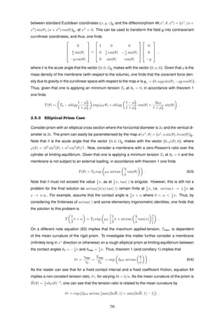
![0.5 1 1.5
δb
1.4
1.6
1.8
2
2.2
2.4
2.6
2.8
δτ
0.4 0.5 0.6 0.7 0.8 0.9 1
βδ
1.4
1.6
1.8
2
2.2
2.4
2.6
2.8
δτ
Figure 21: Tension ratio against δb and βδ.
To investigate this matter further plot the tension ratio, δτ, against δb, and, as the mean curvature
is not constant at the contact region, plot the tension ratio against the critical parametric-latitude,
βδ. Figure 21 is calculated with µF = 1
2 and 1
2 ≤ δb ≤ 3
2 . It shows that, for a fixed contact interval,
as δb and the critical parametric-latitude increases, i.e. as the mean curvature of the contact region
increases, the tension ratio also increases. This is an intuitive result as the curvature of the contact
region increases, the normal reaction force on the membrane also increases, which intern leads to
higher frictional force, and thus, a higher tension ratio. Now, this is a fascinating result as this effect
cannot be observed with the ordinary capstan equation.
2.5.4 Right-Circular Cone Case
Consider a right-circular cone with a 2α-aperture (i.e. angle between two generatrix lines). The
cone can easily be parameterised by the map σ(x1
, θ) = (x1
, x1
tan(α) sin(θ), x1
tan(α) cos(θ))E.
Now, consider a membrane with a zero-Poisson’s ratio over the cone, which resides in sufficiently
away from the apex, at limiting equilibrium. Given that one is applying a minimum tension T0 at
θ0 = 0, in accordance with theorem 2 one finds
T(θ) = T0 exp (µF cot[α] sin (sin[α]θ)) . (65)
As the aperture becomes infinitesimally small, i.e. 2α ≈ 0, one expects the cone to resemble a
cylinder with an infinitesimally small radius. Thus, in the limit α → 0, equation 65 reduces to
T(θ) = T0 exp (µF θ) ,
which is just the ordinary capstan equation 62. Also, when the aperture is π, one gets a (flat-)
Euclidean plane, i.e. (c, y, z)E where c > 0. Thus, in the limit α → 1
2 π, equation 65 reduces to
T(θ) = T0 ,
which is a logical result as this represent a membrane on a flat surface being pulled tangentially
and independent of any transverse effects. To visualise consider a straight rope under tension, i.e.
Tmax = T0.
77](https://image.slidesharecdn.com/a24f3df3-5be8-40a0-a0ff-910a71f94372-170108131508/85/PhDKJayawardana-83-320.jpg)
![2.6 Comparison Against the Works of Kikuchi and Oden
In this section, we extend Kikuchi and Oden’s [102] model for Coulomb’s law of static friction to
curvilinear coordinates, and we conduct several numerical examples to compare the results against
our generalised capstan equation.
Let Ω ⊂ R3
be a simply connected open bounded domain and let ∂Ω = ∂Ω0 ∪∂Ωf ∪∂ΩT be the suf-
ficiently smooth boundary of the domain, where all meas(∂Ω0; R2
), meas(∂Ωf ; R2
), meas(∂ΩT ; R2
) >
0. Now, let ¯X : Ω → E3
be a diffeomorphism where ¯X(x1
, x2
, x3
) = σ(x1
, x2
) + x3
N(x1
, x2
) and
σ ∈ C2
(∂Ω0; R2
) is an injective immersion.
Now, assume that Ω describes the domain of an elastic body such that ∂Ω0 describes the region
where the body is in contact with a rough rigid surface, ∂Ωf describes the stress free boundary
and ∂ΩT describes the boundary with traction. Let v ∈ C2
(Ω; R3
) be the displacement field of
the body. Given that f ∈ C0
(Ω; R3
) is an external force density field and τ0 ∈ C0
(∂Ω0; R3
) is
a traction field (i.e. applied boundary stress) at ∂ΩT , one can express the equations of equilib-
rium in curvilinear coordinates as ¯iTi
j (v) + fj = 0, where Tij
(v) = Aijkl
Ekl(v) is second Piola-
Kirchhoff stress tensor, Ekl(v) = 1
2 ( ¯ivj + ¯jvi) is linearised Green-St Venant strain tensor and
Aijkl
= λgij
gkl
+ µ(gik
gjl
+ gil
gjk
) is the isotropic elasticity tensor in curvilinear coordinates. The
trivial boundary conditions are ¯niTi
j (v) = 0 on ∂Ωf and ¯niTi
j (v) = τ0j on ∂ΩT , where ¯n is the unit
outward normal to ∂Ω.
But what about the boundary conditions at the boundary ∂Ω0? To investigate this matter further
recall Kikuchi and Oden’s [102] model for Coulomb’s law of static friction from Section 1.11. Now,
assume that ¯X is constructed such that v3
describes the normal displacement and vβ
describe the
tangential displacements at the boundary ∂Ω0. Noticing that T3
3 (v)|∂Ω0 = −σn(v) simply re-express
the friction equation (44) in curvilinear coordinates to obtain
u3
|∂Ω+
0
= 0 ,
Tβ
3 (v)|∂Ω+
0
=
−
νF (g33)
1
2
vβ
(vαvα)
1
2
T3
3 (v)|∂Ω+
0
, if (vαvα
)
1
2 |∂Ω+
0
≥ ε ,
−
νF (g33)
1
2
vβ
ε
T3
3 (v)|∂Ω+
0
, if (vαvα
)
1
2 |∂Ω+
0
< ε ,
(66)
where ∂Ω+
0 = limx3→0+ Ω, νF is the coefficient of friction with respect to Coulomb’s law of static
friction, T3
3 (v)|∂Ω+
0
is the purely normal stress, Tβ
3 (v)|∂Ω+
0
are the shear stresses and ε > 0 is the
regularisation parameter. Note that in this framework one has g33 = 1. Despite the fact that one is
working with linear elasticity, the above equations makes this problem inherently nonlinear. Thus, to
find numerical solutions, employ Newton’s method for nonlinear systems (see chapter 10 of Burden
et al. [30]).
Note that the above set of equations depends on the physical properties of the elastic body. Now,
recall the standard friction law (52). This is a very simple law that does not depend on any me-
chanical and geometrical properties of the body in question. Thus, under what conditions does
78](https://image.slidesharecdn.com/a24f3df3-5be8-40a0-a0ff-910a71f94372-170108131508/85/PhDKJayawardana-84-320.jpg)
![Coulomb’s law satisfy the standard friction law?
To investigate this matter further consider the map of a rigid semi-prism (x1
, a sin(x2
), b cos(x2
))E,
where x2
∈ [−1
2 π, 1
2 π], a is the horizontal radius and b is the vertical radius. Now, assume that an
elastic body is over this prism and one is applying a traction τ0 at x2
= −1
2 π and a traction τmax
at x2
= 1
2 π. Also, assume that the cylinder is rough and the coefficient of friction between the
prism and the body in question is 1
2 . Assume further that the body in question is of thickness h,
infinitely long and in contact with an infinitely long semi-prism. This leads to the following map of
the unstrained configuration,
¯X(x1
, x2
, x3
) = (x1
, a sin(x2
), b cos(x2
))E + x3
(ϕ(x2
))−1
(0, b sin(x2
), a cos(x2
))E ,
where ϕ(x2
) = (b2
sin2
(x2
) + a2
cos2
(x2
))
1
2 , x1
∈ (−∞, ∞), x2
∈ (−1
2 π, 1
2 π) and x3
∈ (0, h). With
some calculations, one finds that the covariant metric tensor is (gij) = diag(1, ( ¯ψ2)2
, 1) and Christof-
fel symbols of the second kind are
¯Γ2
22 = ( ¯ψ2)−1
∂2
¯ψ2 ,
¯Γ2
23 = ( ¯ψ2)−1
∂3
¯ψ2 ,
where ¯ψ2 = ϕ(x2
)+x3
ab(ϕ(x2
))−2
. Now, let v = (0, v2
(x2
, x3
), v3
(x2
, x3
)) be the displacement field
of the elastic body and let δv = (0, δv2
(x2
, x3
), δv3
(x2
, x3
)) be a perturbation of the displacement
field. Thus, with some calculations, one finds that covariant derivatives are
¯2v2
= ∂2v2
+ ¯Γ2
22v2
+ ¯Γ2
23v3
,
¯2v3
= ∂2v3
− ( ¯ψ2)2 ¯Γ2
23v2
,
¯3v2
= ∂3v2
+ ¯Γ2
23v2
,
¯3v3
= ∂3v3
.
Now, with relative ease, one can express the governing equations as
(λ + µ)∂2 ¯ivi
+ µ ¯∆v2
= 0 ,
(λ + µ)∂3 ¯ivi
+ µ ¯∆v3
= 0 ,
(λ + µ)∂2 ¯iδvi
+ µ ¯∆δv2
= 0 ,
(λ + µ)∂3 ¯iδvi
+ µ ¯∆δv3
= 0 .
Eliminating x1
dependency one can express the remaining boundaries as
∂ΩNew
= ∂ΩNew
0 ∪ ∂ΩNew
f ∪ ∂Ω
New
T0
∪ ∂Ω
New
Tmax
,
where
∂ΩNew
0 = {(−
1
2
π,
1
2
π) × {0}} ,
∂ΩNew
f = {(−
1
2
π,
1
2
π) × {h}} ,
∂ΩNew
T0
= {{−
1
2
π} × (0, h)} ,
79](https://image.slidesharecdn.com/a24f3df3-5be8-40a0-a0ff-910a71f94372-170108131508/85/PhDKJayawardana-85-320.jpg)
![∂ΩNew
Tmax
= {{
1
2
π} × (0, h)} .
Thus, the boundary conditions reduce to
v3
|∂Ω
New
0
= 0 (zero-Dirichlet) , (67)
(λ + 2µ) ∂2v2
+ ¯Γ2
22v2
+ ¯Γ2
23v3
+ λ∂3v3
|∂Ω
New
T0
= τ0 (traction) ,
(λ + 2µ) ∂2v2
+ ¯Γ2
22v2
+ ¯Γ2
23v3
+ λ∂3v3
|∂Ω
New
Tmax
= τmax (traction) ,
( ¯ψ2)2
∂3v2
+ ∂2v3
|∂ΩNew
f ∪∂ΩNew
T0
∪∂ΩNew
Tmax
= 0 (zero-Robin) ,
λ ∂2v2
+ ¯Γ2
22v2
+ ¯Γ2
23v3
+ (λ + 2µ)∂3v3
|∂Ω
New
f
= 0 (zero-Robin) ,
δv2
|∂Ω
New
f ∪∂ΩNew
T0
∪∂ΩNew
Tmax
= 0 ,
δv3
|∂ΩNew = 0 .
Note that condition (67) arises due to the fact that the body is in contact with a rigid boundary. In
chapter 4 we examine a more complicated example where this condition is no longer true.
Now, with some more calculations, one can find the fiction laws governing the boundary conditions
at the boundary ∂Ω
New
0 , which are:
If ¯ψ2|v2
||∂ΩNew
0
≥ , then
µ ¯ψ2∂3v2
+ νF sign(v2
)T3
3 (v) |∂ΩNew
0
= 0 ;
If ¯ψ2|v2
||∂ΩNew
0
< , then
µ ¯ψ2∂3δv2
+ νF
−1 ¯ψ2v2
T3
3 (δv) + νF
−1 ¯ψ2δv2
T3
3 (v) + µ ¯ψ2∂3v2
+ νF
−1 ¯ψ2v2
T3
3 (v) |∂ΩNew
0
= 0 ,
where T3
3 (v) = λ(∂2v2
+ ¯Γ2
22v2
+ ¯Γ2
23v3
) + (λ + 2µ)∂3v3
.
Despite the fact that the original problem is three-dimensional, as a result of problem’s invariance
in the x1
direction, it is now to a two-dimensional problem. Now, the domain resides in the set
{(x2
, x3
) | (x2
, x3
) ∈ [−1
2 π, 1
2 π] × [0, h]}. We are fully aware that Kikuchi and Oden’s [102] model is
only defend for bounded domains; however, we later show that the reduced two-dimensional prob-
lem is numerically sound.
To conduct numerical experiments we use the second-order-accurate finite-difference method in
conjunction with Newton’s method for nonlinear systems, i.e. given that vm and δvm are mth
iterative
solutions of the problem obtained by the finite-difference method, we assert that vm+1 = vm+δvm is
the updated solution, and we follow this iterative scheme such that δvm converges to zero in the limit
m → ∞. Another issue we must tackle is the discretisation of the (reduced two-dimensional) do-
main. As we are dealing with curvilinear coordinates, there is an inherit grid dependence. To be pre-
cise, it is approximately ψ0∆x2
≤ ∆x3
, ∀ ψ0 ∈ { ¯ψ2(x2
, x3
) | x2
∈ [−1
2 π, 1
2 π] and x3
∈ [0, h]}, where
∆xj
is a small increment in xj
direction. For our purposes we use ∆x2
= 1
N−1 and ψ0 = ¯ψ2(1
4 π, h),
where N = 250. Finally, we must define a terminating condition. For this we terminate our iterating
80](https://image.slidesharecdn.com/a24f3df3-5be8-40a0-a0ff-910a71f94372-170108131508/85/PhDKJayawardana-86-320.jpg)
![process given that the condition |1 − (||vm|| 2 + ||δvm|| 2 )−1
(||vm+1|| 2 + ||δvm+1|| 2 )| < 10−10
is
satisfied, where |v| 2 = ([norm(v2
, 2)]2
+ [norm(v3
, 2)]2
)
1
2 and norm(·, 2) is Matlab 2-norm of matrix
[201]. Note that for all our examples we fix the values νF = 1
2 , τ0 = 1 and a = 2.
-2
-1.5
-1
-0.5
2
0
0.5
1
1.5
AzimuthalDisplacement
×10-3
Radius
1.5
2
θ
101 -1-2
-9
-8
-7
-6
-5
1
-4
-3
-2
-1
0
RadialDisplacement
×10-4
Radius
1.5
-2
θ
-102 12
Figure 22: Displacement field of the modified Kikuchi and Oden’s model.
Figures 22 and 23 are calculated with the values of τmax = 1, b = 2, h = 1, E = 103
, ν = 1
4 , ε = 10−5
and with a grid of 250 × 41 points. Figure 22 shows the azimuthal (i.e v2
) and the radial (i.e v3
)
displacements. The maximum azimuthal displacements are observed at x2
= ±1
2 π, with respective
azimuthal displacements of v2
= ±1.72 × 10⁻³
. The maximum radial displacement is observed at
x2
= ±1
2 π, with a radial displacement of v3
= −8.24 × 10⁻⁴
.
-2 -1 0 1 2
θ
-1
-0.8
-0.6
-0.4
-0.2
0
0.2
0.4
0.6
0.8
1
-1,+1=Slip,0=NoSlip
Figure 23: Slip and stick regions of the modified Kikuchi and Oden’s model.
Figure 23 shows the behaviour of the elastic body at the boundary ∂Ω
New
0 . It shows that in the
region [−1
2 π, −0.0694] the body slid in the negative (i.e. decreasing) azimuthal direction, and in the
region [0.0694, 1
2 π] the body slid in the positive (i.e. increasing) azimuthal direction. The region
81](https://image.slidesharecdn.com/a24f3df3-5be8-40a0-a0ff-910a71f94372-170108131508/85/PhDKJayawardana-87-320.jpg)
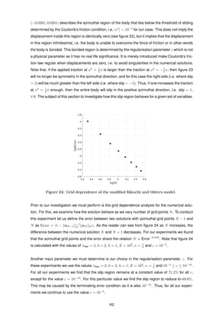
![1 1.5 2 2.5 3
δτ
0
10%
20%
30%
40%
50%
60%
70%
80%
90%
100%
Slip
Limiting Equilibrium
Coulombs
Figure 25: Slip for δτ = τmax/τ0.
Figure 25 shows how close the elastic body is to limiting equilibrium for varying tension ratio, δτ. For
these experiments we assert that δτ ∈ {1, 5
4 , 6
4 , 7
4 , 2, 9
4 , 10
4 , 11
4 }, δb = 1, h = 1, E = 103
and ν = 1
4 . In
figure 25 we see that as the tension ratio increases, the elastic body gets closer and closer to fully
debonding. In fact, when δτ = 11
4 , our elastic body is fully debonded from the rigid foundation and
sliding in the positive x2
direction. To compare it against the capstan equation we invoke corollary
1 with δτ = 11
4 , which implies that the capstan coefficient of friction is µF = 0.322, regardless of the
Poisson’s ratio of the body. This result implies that the capstan coefficient of friction is an underesti-
mate of Coulomb’s coefficient of friction, i.e. µF ≤ νF . Note that capstan equation underestimating
the actual coefficient of friction is a documented phenomenon in the literature [134].
-3 -2 -1 0 1 2 3
y-axis
0.5
1
1.5
2
2.5
3
3.5
z-axis
Low Critical Parametric-Latitude: a = 2, b = 1.5
-3 -2 -1 0 1 2 3
y-axis
0.5
1
1.5
2
2.5
3
3.5
z-axis
High Critical Parametric-Latitude: a = 2, b = 2.5
Figure 26: Schematic representations of the reduced two-dimensional domain for the h =
1, a = 2, and b = 3
2 and b = 5
2 cases.
Figure 27 shows how close the elastic body is to limiting equilibrium for a set of vertical radii of the
contact region, δb = b/a. For these experiments we assert that δτ = 2, δb ∈ { 5
10 , 6
10 , 7
10 , 8
10 , 9
10 , 1, 11
10 ,
12
10 , 13
10 , 14
10 , 15
10 } (see figure 26), h = 1, E = 103
and ν = 1
4 . Figure 27 implies that as δb increases,
the modified Kikuchi and Oden’s model moves away from limiting equilibrium, i.e. as the critical
parametric-latitude increases, the normal reaction force of the body increases, which intern leads to
83](https://image.slidesharecdn.com/a24f3df3-5be8-40a0-a0ff-910a71f94372-170108131508/85/PhDKJayawardana-89-320.jpg)
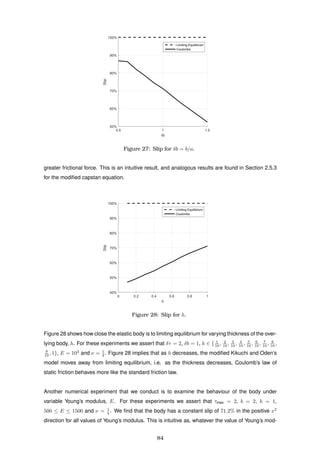
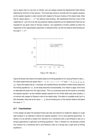
![Then, in Section 2.6, we extended Kikuchi and Oden’s [102] model for Coulomb’s law of static
friction to curvilinear coordinates. There, we conducted numerical experiments to see how close
Coulomb’s law of static friction is to the ordinary friction law (52) is, in curvilinear coordinates. To
do this we modelled an elastic body over a rigid rough prism with an elliptical cross section. Our
numerical results indicate the following (for a fixed coefficient of friction): (i) capstan coefficient of
friction is an underestimate of Coulomb’s coefficient of friction, i.e. µF ≤ νF , (ii) as the critical
parametric-latitude of the contact region increases, one require a larger force to debond the body,
a result that coincides with the modified capstan equation, (iii) as the thickness of the body de-
creases, one require a larger force to debond the body, yet this force is still an underestimate to
what is predicted by the modified capstan equitation, (iv) Young’s modulus of the body does not
affect the governing equation of the contact region, a result that coincides with the ordinary capstan
equation, and (v) as Poisson’s ratio of the body increases, one requires a larger force to debond
the body. The last result implies that incompressible elastic bodies such as rubber tend to be more
difficult to debond from a rigid surface relative to a compressible object (e.g. piece of marshmallow)
with the same coefficient of friction acting on the contact region. Now, this is a surprising result as
this behaviour is not predicted by the modified capstan equation as the modified capstan equation
is invariant with respect to Poisson’s ratio of the body, for the given problem.
Our analysis shows that modelling friction is not a well understood problem. This is due to the fact
that for the same value of coefficient of friction different models predict vastly different results, such
as different limiting equilibriums. This further implies that, if one’s goal is to find the coefficient of
friction for a given set of input values, then different models predict a different coefficient of friction
for the same set of input values, i.e. coefficient of fiction is dependent on the friction model that is
being used to calculate it.
Note that the work we presented in Sections 2.3 and 2.4 has real life significance as it can be easily
be applied to cable drive devices (see Section 1.6). Consider an electronic robotic hand, where
precision is significant, and consider a tendon running over outer part of a joint. Given that the joint
has a noncircular crosses section, hypothetically assume it is elliptical, one can easily calculate the
force required to overcome friction with the use of equation (63), or using theorem 1 for a more
complicated geometry.
86](https://image.slidesharecdn.com/a24f3df3-5be8-40a0-a0ff-910a71f94372-170108131508/85/PhDKJayawardana-92-320.jpg)
![3 Shells Supported by Elastic foundations: Boundary Forms
to Model the Bonded Case
Abstract
In this chapter we derive a theory for bonded shells on elastic foundations. We show that, if the
diffeomorphism ¯X ∈ C2
(¯Ω; E3
) describes the unstrained configuration of the foundation and the
injective immersion σ ∈ C3
(¯ω; E3
) describes the unstrained configuration of the overlying shell,
where Ω ⊂ R3
is a connected open bounded domain that satisfies the segment condition with a
uniform-C1
(R3
; R2
) boundary ∂Ω such that ω, ∂Ω0 ⊂ ∂Ω, ¯ω ∩ ¯∂Ω0 = Ø, meas(∂Ω0; R2
) > 0, and
ω ⊂ R2
is a connected open bounded plane that satisfies the segment condition with a uniform-
C1
(R2
; R) boundary ∂ω, with f ∈ L2
(Ω), f0 ∈ L2
(ω) and τ0 ∈ L2
(∂ω), then there exists a unique
field u ∈ VS (ω, Ω) such that u is the solution to the minimisation problem
J(u) = min
v∈VS (ω,Ω)
J(v) ,
where
VS (ω, Ω) = {v ∈ H1
(Ω) | v|ω ∈ H1
(ω)×H1
(ω)×H2
(ω), v|∂Ω0 = 0, ∂β(v3
|ω)|∂ω = 0 ∀β ∈ {1, 2}} ,
J(u) =
Ω
1
2
Aijkl
Eij(u)Ekl(u) − fi
ui dΩ
+
ω
1
2
Bαβγδ
h αβ(u) γδ(u) +
1
3
h3
ραβ(u)ργδ(u) − hfi
0ui dω −
∂ω
hτi
0 ui d(∂ω) ,
and where A is the elasticity tensor and E(·) is the stain tensor of the foundation, and B is the
elasticity tensor, (·) is half of the change in first fundamental form tensor, ρ(·) is the change
in second fundamental form tensor and h is the thickness of the shell. In particular, the unique
minimiser u is also a critical point in (VS (ω, Ω), J(·)).
3.1 Introduction
In this chapter we develop a theory for elastic shells that are bonded to elastic foundations (see fig-
ure 30). In the current literature there exists a limited number of publications on the study of plates
and films that are bonded to elastic foundations (see sections 1.7 and 1.10), yet there exists no
comprehensive theory to describe the behaviour of shells that are supported by elastic foundations.
In Section 3.2, we begin by modifying the linear Koiter’s shell equations to describe the behaviour of
a shell if it is in contact with a three-dimensional elastic body by considering a technique that is used
in the derivation of surface Cauchy-Bourne model [89]. Then, in Section 3.3, we explicitly derive the
governing equations and the boundary conditions for the general case. In Section 3.4 we treat the
bonded shell as a boundary form of the elastic foundation, which is analogous to the work of Necas
et al. [144]. Then, we use a combination of Ciarlet’s [38], and Badiale and Serra’s [13] work to prove
the existence and the uniqueness of solutions, and then conduct some numerical experiments in
Section 3.5. In Section 3.6 we extend Baldelli and Bourdin’s [16] model for bonded films on elastic
foundations to curvilinear coordinates and show how numerical solutions fair against our numerical
model, with respect to the bonded two-body elastic problem. To conclude our numerical analysis, in
Section 3.7, we analyse how effective our model is at approximating the bonded two-body problem.
Finally, in Section 3.8, we conclude this chapter with our findings and some notable applications.
87](https://image.slidesharecdn.com/a24f3df3-5be8-40a0-a0ff-910a71f94372-170108131508/85/PhDKJayawardana-93-320.jpg)
![R3
ω
Ω
E3
Shell
Foundation
σ(ω)
_
X(Ω)
Figure 30: Two-Dimensional schematic representation of the reference configuration of an
overlying shell bonded to an elastic foundation.
3.2 Derivation
Consider an unstrained static three-dimensional elastic body described by the diffeomorphism
¯X ∈ C2
(¯Ω; E3
), where Ω ⊂ R3
is a connected open bounded domain that satisfies the segment
condition with a uniform-C1
(R3
; R2
) boundary. Now, assume that on a part of body’s boundary,
with a positive mean-curvature with respect to the unit outward normal and described by the injec-
tion σ ∈ C3
(¯ω; E2
) where ω ⊂ R2
is a connected open bounded plane that satisfies the segment
condition with a uniform-C1
(R2
; R) boundary, lies an elastic shell with the same curvature and the
same physical form as the given surface, which is also bonded to the surface. Now, recalling the
shell equations form from Section 1.4 it is clear that one cannot directly apply the shell equations
to describe the behaviour of an overlying shell for the following reasons: (i) if one applies the
shell equations as it stands, they imply that both the shell and the elastic body occupy the region
¯ω × [0, −1
2 h], which is not physically viable, and (ii) one may displace the map σ by 1
2 hN amount,
where N unit outward normal at the contact region, but this violates the condition that the lower
(and the upper) surface of the shell is stress free. Also, the latter condition is problematic as when
trying to prove the existence and the uniqueness of the solutions as one will not be able to express
the governing equations of shell as a boundary form. Thus, one must consider an alternative way
of tackling this problem.
To do so, consider the following: assume an overlying shell whose lower-surface is parameterised
by the sufficiently smooth injection σ(x1
, x2
). Thus, any surface of the shell can be parameterised
by the map ϕ(x1
, x2
) = σ + ξN(x1
, x2
), ∀ ξ ∈ [0, h], where h is the thickness of the shell. Now,
consider the normal (not the unit normal) of the map ϕ(x1
, x2
), which can be expressed as
∂1ϕ × ∂2ϕ = (∂1σ × ∂2σ) 1 − ξF α
[II]α + ξ2
F 1
[II]1F 2
[II]2 − F 2
[II]1F 1
[II]2 , ∀ ξ ∈ [0, h] .
For our analysis we require the normal to any surface of the overlying shell, ∂1ϕ × ∂2ϕ, to be the
same sign as the normal to the lower-surface, ∂1σ × ∂2σ, and to be almost the same magnitude as
the normal to the lower-surface, for all ξ. Now, this can be achieved by asserting the following:
Assertion 1. Let the map σ ∈ C3
(¯ω; E2
) describes the lower-surface of an unstrained shell,
where ω ⊂ R2
is a connected open bounded plane that satisfies the segment condition with
88](https://image.slidesharecdn.com/a24f3df3-5be8-40a0-a0ff-910a71f94372-170108131508/85/PhDKJayawardana-94-320.jpg)
![a uniform-C1
(R2
; R) boundary. Given that the thickness of the shell is h, we assert that
0 ≤ h2
F 1
[II]1 F 2
[II]2 − F 2
[II]1 F 1
[II]2 < −
1
2
hF α
[II]α 1 , ∀ (x1
, x2
) ∈ ¯ω ,
i.e. the lower-surface of the shell is not hyperbolic and it is a surface of positive mean curva-
ture, and the thickness of the shell is sufficiently small .
Note that positive mean-curvature (i.e. 1
2 F α
[II]α < 0) is essential in our numerical modeling in Section
3.5, 3.6 and 3.7. Also, assertion 1 is essential in chapter 4, where we no longer assert that the shell
is bonded to the elastic body.
Now, assume that one is dealing with shell with a thickness 2h, i.e. the energy functional is J2h(w) =
J(w, 2h, 2
3 h3
), where w describes the displacement field with respect to the mid-surface. Given
that this shell satisfies the conditions described by assertion 1, its upper and lower half maybe
approximated by dividing energy functional of the shell by 2. To be more precise, if J2h(w) =
Jupper(w) + Jlower(w), then assume that 1
2 J2h(w) ≈ Jupper(w) ≈ Jlower(w). This is due to the fact
that we asserted that the lower-surface of the shell is not hyperbolic and it is a surface of positive
mean curvature, and the thickness of the shell is sufficiently small, and thus, these conditions imply
that the change in the second fundamental form tensor is small for infinitesimal deformations, i.e.
h2
F γ
[II]αF α
[II]γ ≈ 0 =⇒ h2
ρα
γ (w)ργ
α(w) ≈ 0. Thus, one can expect J2h(w) to behave approximately
linear in h, despite its cubic h dependence. Now, take the upper half and assert that this is the
form of an overlying shell equation: this is a similar logical process that is used in the derivation of
surface Cauchy-Bourne model [89]. Thus, we come to our second hypothesis of this thesis:
Hypothesis 2. The energy functional of an overlying shell with a thickness h is
J(u)shell =
ω
1
2
Bαβγδ
h αβ(u) γδ(u) +
1
3
h3
ραβ(u)ργδ(u) − hfi
ui dω −
∂ω
hτi
0 ui d(∂ω) ,
given that the shell satisfies the conditions from assertion 1, where u describes the dis-
placement field with respect to the lower-surface, the map σ ∈ C3
(¯ω; E2
) describes the lower-
surface of an unstrained shell, and ω ⊂ R2
is a connected open bounded plane that satisfies
the segment condition with a uniform-C1
(R2
; R) boundary.
J2h
Jupper
x3
= 0
Jlower
Jshell
Jupper
x3
= 0
Figure 31: Two-Dimensional schematic representation of hypothesis 2.
Note that there are two things differ from the ordinary shell equations and our overlying shell equa-
tions: the choice in the displacement field and the fraction that proceeding the h3
term. In the
89](https://image.slidesharecdn.com/a24f3df3-5be8-40a0-a0ff-910a71f94372-170108131508/85/PhDKJayawardana-95-320.jpg)
![ordinary shell equations the displacement field describes the displacement from the mid-surface
and, for a shell with a thickness h, fraction that proceeding the h3
term is 1
12 . But, in our overlying
shell equations the displacement field describes the displacement from the lower-surface and, for a
shell with a thickness h, fraction that proceeding the h3
term is 1
3 . Why does this make sense? Well,
consider a thin overlying body. Let the diffeomorphism Θ = σ + x3
N ∈ C2
(¯ω × [0, h]; R3
) describes
the unstrained configuration of this body and let u(x1
, x2
) be the displacement field with respect to
the lower-surface, i.e. u is the displacement field with respect to the contact surface. Now, con-
sider the pure-stretching case with the displacement field (u1
, u2
, 0), an external force density field
(f1
, f2
, 0) and a traction field (τ1
0 , τ2
0 , 0). For this case one can express the energy functional as
J(u) =
ω
1
2
hBαβγδ
αβ(u) γδ(u) − hfα
uα dω −
∂ω
hτα
0 uα d(∂ω)
= lim
u3,ρ(u)→0
J(u)shell .
Now, consider the pure-bending case with the displacement field ( − x3
∂1
u3, −x3
∂2
u3, 0), an exter-
nal force density field (f1
, f2
, 0) and a traction field (τ1
0 , τ2
0 , 0). For this case one can express the
energy functional as
J(u) =
ω
1
2
1
3
h3
Bαβγδ
ραβ(u)ργδ(u) − hf3
u3 dω −
∂ω
hτ3
0 u3 d(∂ω)
= lim
u1,u2, (u)→0
J(u)shell ,
where f3
= 1
2 h αfα
and τ3
0 = 1
2 h ατα
0 . Thus, if one considers the pure-stretching and the pure-
bending case separately for a thin overlying body where the displacement field is approximated by
the displacement with respect to the contact region, then hypothesis 2 perfectly coincides with the
each respective energy functionals. Can the reader now see why hypothesis 2 makes sense?
Now, with hypothesis 2 one can finally express the equations for a bonded shell on an elastic
foundation, which leads to the following theorem:
Theorem 3. Let Ω ⊂ R3
be a connected open bounded domain that satisfies the segment
condition with a uniform-C1
(R3
; R2
) boundary ∂Ω such that ω, ∂Ω0 ⊂ ∂Ω, where ¯ω ∩ ¯∂Ω0 = Ø
with meas(∂Ω0; R2
) > 0, and let ω ⊂ R2
be a connected open bounded plane that satisfies
the segment condition with a uniform-C1
(R2
; R) boundary ∂ω. Let ¯X ∈ C2
(¯Ω; E3
) be a dif-
feomorphism and σ ∈ C3
(¯ω; E3
) be an injective immersion. Let f ∈ L2
(Ω), f0 ∈ L2
(ω) and
τ0 ∈ L2
(∂ω). Then there exists a unique field u ∈ VS (ω, Ω) such that u is the solution to the
minimisation problem
J(u) = min
v∈VS (ω,Ω)
J(v) ,
where
VS (ω, Ω) = {v ∈ H1
(Ω) | v|ω ∈ H1
(ω)×H1
(ω)×H2
(ω), v|∂Ω0 = 0, ∂β(v3
|ω)|∂ω = 0 ∀β ∈ {1, 2}} ,
J(u) =
Ω
1
2
Aijkl
Eij(u)Ekl(u) − fi
ui dΩ
+
ω
1
2
Bαβγδ
h αβ(u) γδ(u) +
1
3
h3
ραβ(u)ργδ(u) − hfi
0ui dω −
∂ω
hτi
0 ui d(∂ω) .
In particular, the unique minimiser u is also a critical point in (VS (ω, Ω), J(·)).
90](https://image.slidesharecdn.com/a24f3df3-5be8-40a0-a0ff-910a71f94372-170108131508/85/PhDKJayawardana-96-320.jpg)
![Proof. See Section 3.4.
Note that by v|∂Ω0 and v|ω we mean in a trace sense.
What does theorem 3 mean? Well, it means that for some well-posed normal and tangential forc-
ings, and tractions acting on a shell with a thickness h that is bonded to an elastic foundation,
J(·) has a unique weak solution in the set VS (ω, Ω). This weak solution is sufficient for finding
finite-element solutions. For a comprehensive study of finite-element modelling of similar problems
please consult chapter 4 of Kikuchi and Oden [102]. However, one requires higher regularity results
to prove the existence of classical solutions. This problem is a subject of discussion in Section 5.3.
Also, note that due to the conditions ∂β(u3
|ω)|∂ω = 0, ∀ β ∈ {1, 2}, external moments cannot be
applied to the boundary of the shell.
Theorem 3 is also valid for the weaker conditions f ∈ L
6
5 (Ω) (see theorem 3.9-2 of Ciarlet [39]),
fα
0 ∈ Lr
(ω) ∀ α ∈ {1, 2} and f3
0 ∈ L1
(ω), where r > 1 (see theorem 4.4-2 of Ciarlet [39]). However,
we are unfamiliar with the proof, and thus, we refrain from asserting these weaker conditions herein.
Note that the displacement u restricted to the boundary ω should be understood in the context of
the statement. For example, by ω
u dω we mean that ω
u|ω dω, where u|ω in a trace sense. We
often neglect the term |ω for convenience.
3.3 Equations of Equilibrium
For this section we assume that u ∈ C2
(Ω; R3
) with uα
|ω ∈ C3
(ω) and u3
|ω ∈ C4
(ω), and use
theorem 3 to derive a set of governing equations and boundary conditions for our problem.
3.3.1 Governing Equations of the Elastic Foundation
¯iTi
j (u) + fj = 0 , ∀ j ∈ {1, 2, 3} ,
where Tij
(u) = Aijkl
Ekl(u) is second Piola-Kirchhoff stress tensor, Eij(u) = 1
2 (gik
¯juk
+gjk
¯iuk
)
is linearised Green-St Venant stress tensor, Aijkl
= ¯λgij
gkl
+ ¯µ(gik
gjl
+ gil
gjk
) is the isotropic
elasticity tensor, ¯λ = (1 − ¯ν − 2¯ν2
)−1
¯ν ¯E is first Lam´e’s parameter, ¯µ = 1
2 (1 + ¯ν)−1 ¯E is second
Lam´e’s parameter, ¯E is Young’s modulus and ¯ν is Poisson’s ratio of the elastic foundation, and f is
an external force density field acting on the elastic foundation.
3.3.2 Boundary Conditions of the Elastic Foundation
u|∂Ω0
= 0 , (68)
¯niTi
j (u)|{∂Ω{ω∪∂Ω0}} = 0 , ∀ j ∈ {1, 2, 3} , (69)
where ¯n is the unit outward normal to the boundary ∂Ω in curvilinear coordinates. Dirichlet boundary
condition (68) is often referred to as the zero-displacement boundary condition and Robin boundary
condition (69) is often referred to as the stress free boundary condition.
91](https://image.slidesharecdn.com/a24f3df3-5be8-40a0-a0ff-910a71f94372-170108131508/85/PhDKJayawardana-97-320.jpg)
![3.3.3 Governing Equations of the Overlying Shell
ατα
β (u) +
2
3
h2
F α
[II]β γηγ
α(u) +
1
3
h2
γF α
[II]β ηγ
α(u) −
1
h
Tr(T3
β (u)) + f0β = 0 , ∀ β ∈ {1, 2} ,
F γ
[II]ατα
γ (u) −
1
3
h2
α ( γηαγ
(u)) +
1
3
h2
F δ
[II]αF α
[II]γ ηγ
δ (u) −
1
h
Tr(T3
3 (u)) + f03 = 0 ,
where ταβ
(u) = Bαβγδ
γδ(u) is the stress tensor, ηαβ
(u) = Bαβγδ
ργδ(u) negative of the change in
moments density tensor,
αβ(u) =
1
2
( α(uβ|ω) + β(uα|ω)) − F[II]αβ(u3
|ω)
is half of the change in first fundamental form tensor,
ραβ(u) = α β(u3
|ω) − F[II]αγF γ
[II]β (u3
|ω) + F[II]βγ α(uγ
|ω) + F[II]αγ β(uγ
|ω) + ( αF[II]βγ) (uγ
|ω)
the change in second fundamental form tensor,
Bαβγδ
=
2λµ
λ + 2µ
Fαβ
[I] Fγδ
[I] + µ(Fαγ
[I] Fβδ
[I] + Fαδ
[I] Fβγ
[I] )
is the isotropic elasticity tensor, λ = (1 − ν − 2ν2
)−1
νE is first Lam´e’s parameter, µ = 1
2 (1 + ν)−1
E
is second Lam´e’s parameter, E is Young’s modulus and ν is Poisson’s ratio of the overlying bonded
shell, Tr(T3
j (u)) = T3
j (u)|ω is the normal stresses of the foundation at the contact region and f0 is
an external force density field action on the overlying bonded shell.
3.3.4 Boundary Conditions of the Overlying Shell
nατα
β (u) +
2
3
h2
nγF α
[II]β ηγ
α(u) |∂ω = τ0β , ∀ β ∈ {1, 2} ,
−
1
3
h2
nγ αηαγ
(u)|∂ω = τ03 ,
∂β(u3
|ω)|∂ω = 0 , ∀ β ∈ {1, 2} , (70)
where n is the unit outward normal vector to the boundary ∂ω in curvilinear coordinates and τ0 is
an external traction field acting on the boundary of the overlying bonded shell. Neumann boundary
condition (70) is often referred to as the zero-slope boundary condition. Due the zero-slope bound-
ary conditions one cannot apply external moments to the boundary of the shell. If one requires to
apply boundary moments to the shell, then one must assume that ∂β(u3
|ω)|∂ω are unknowns. The
reason that we insist upon the zero-slope boundary conditions is described in Section 5.2.
3.4 Existence and Uniqueness of Solutions
In this section we prove theorem 3, and thus, finally concluding that the model derived in this chap-
ter is a mathematical theory. As we consider the equations of the overlying shell as a boundary
form of the foundation, one may think that we may easily prove the existence and the uniqueness
of solutions of our problem with the use of mathematical techniques for boundary forms put forward
by Necas et al. [144] (see chapter 4 of Necas et al. [144]). However, this is not the case. This is
due to the fact that u requires higher regularity at the boundary than in the interior of the foundation.
Thus, we need to prove the existence and the uniqueness results from scratch. However, we still
92](https://image.slidesharecdn.com/a24f3df3-5be8-40a0-a0ff-910a71f94372-170108131508/85/PhDKJayawardana-98-320.jpg)
![retain the mathematical techniques introduced by Necas et al. [144] in our proof.
Step 1 : Reflexive
The space
W (ω, Ω) = {v ∈ H1
(Ω) | v|ω ∈ H1
(ω)×H1
(ω)×H2
(ω)} ,
equipped with the norm
||v||W (ω,Ω) = ||v1
||2
H1(Ω) +||v2
||2
H1(Ω) +||v3
||2
H1(Ω) +||v1
|ω||2
H1(ω) +||v2
|ω||2
H1(ω) +||v3
|ω||2
H2(ω)
1
2
,
is a Hilbert space, and thus, it is reflexive. This is due to the fact that W (ω, Ω) is a finite Cartesian
product of Hilbert spaces equipped with a product norm consists of a finite collection of the norms
of each respective spaces. This is a trivial result. For comments on the subject please see the proof
of theorem 7.19 of Sokal [182].
Step 2 : Coercive
J(u) is coercive in the set VS (ω, Ω) with respect to the norm || · ||W (ω,Ω). To show this we introduce
Korn’s inequity, which states that there exists a constant C that depends on Ω, ∂Ω0, ¯X, ω, ∂ω and
σ such that
||u||W (ω,Ω) ≤ C ||E(u)||2
L2(Ω) + || (u)||2
L2(ω) + ||ρ(u)||2
L2(ω)
1
2
, ∀ u ∈ VS (ω, Ω) . (71)
This implies that VS (ω, Ω) is a closed subspace of the complete space W (ω, Ω), closed under the
norm || · ||W (ω,Ω). The given Korn’s inequality (71) can be proved by combining and modifying the
proofs of theorems 1.7-2, 1.7-4, 2.6-1 and 2.6-4 of Ciarlet [38]. For an explicit proof please see
Section 3.4.1.
Now, recall the energy functional from theorem 3 and consider that
J(u) =
Ω
1
2
Aijkl
Eij(u)Ekl(u) − fi
ui dΩ
+
ω
1
2
Bαβγδ
h αβ(u) γδ(u) +
1
3
h3
ραβ(u)ργδ(u) − hfi
0ui dω −
∂ω
hτi
0 ui d(∂ω)
≥ C1||E(u)||2
L2(Ω) + C2 h|| (u)||2
L2(ω) +
1
3
h3
||ρ(u)||2
L2(ω)
− C3||f||L2(Ω)||u||L2(Ω) − hC3||f0||L2(ω)||u||L2(ω) − hC4||τ0||L2(∂ω)||u||L2(∂ω)
≥ C5||u||2
W (ω,Ω) − C3||f||L2(Ω)||u||L2(Ω) − hC3||f0||L2(ω)||u||L2(ω) − C6||u||H1(ω)
≥ C5||u||2
W (ω,Ω) − C7||u||W (ω,Ω) − C8||u||H1(ω)
≥ C5||u||2
W (ω,Ω) − C9||u||W (ω,Ω) , ∀ u ∈ VS (ω, Ω) .
This implies that there exist positive constants c1 and c2 that depends on Ω, ∂Ω0, ¯X, ω, ∂ω and σ
such that J(u) ≥ c1||u||2
W (ω,Ω) − c2||u||W (ω,Ω), ∀ u ∈ VS (ω, Ω), i.e. J(u) is coercive. Note that
the constant C1 follows from positive definiteness of the elasticity tensor (lemma 5) and proposition
4, C2 follows form the positive definiteness of the elasticity tensor on a general surface (lemma 6)
and proposition 5. Furthermore, C3 and C4 follow from H¨older inequality (proposition 6), C5 follow
93](https://image.slidesharecdn.com/a24f3df3-5be8-40a0-a0ff-910a71f94372-170108131508/85/PhDKJayawardana-99-320.jpg)
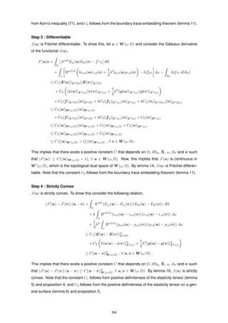
![The above analyses imply that J(·) : VS (ω, Ω) ⊂ W (ω, Ω) → R is a coercive differentiable strictly-
convex functional, where VS (ω, Ω) is complete as subspace of the reflexive Banach space W (ω, Ω)
under the norm || · ||W (ω,Ω). Thus, lemmas 17 and 18 imply that there exists a unique field
u ∈ VS (ω, Ω) such that u is the solution to the minimisation problem J(u) = minv∈VS (ω,Ω) J(v). In
particular, this unique minimiser u is also a critical point in (VS (ω, Ω), J(·)).
As a result of the symmetry (in indices {{1st
, 2nd
}, {3rd
, 4th
}}) of the elasticity tensors A and B, one
can also use Lax-Milgram Theorem (see section 6.2.1 of Evans [63]) to prove the existence and the
uniqueness of solutions. Although, we do not explicitly use the segment condition (definition 6), it
is used in some fundamental theorems that are necessary for our proof to work, as the segment
condition ensures that the boundary of an n-dimensional domain is an (n − 1)-dimensional and that
the boundary remains on one side of the domain.
3.4.1 Korn’s Inequality
In this section we prove Korn’s inequality that we introduced, i.e. equation (71). The following proof
is a combination of the modified versions of Ciarlet’s [38] proofs of theorems 1.7-2, 1.7-4, 2.6-1 and
2.6-4.
Step 1 : Korn’s Inequality Without Boundary Conditions
Consider the space
K(ω, Ω) = {v ∈ L2
(Ω) | v|ω ∈ L2
(ω)×L2
(ω)×H1
(ω), E(v) ∈ L2
(Ω), (v) ∈ L2
(ω), ρ(v) ∈ L2
(ω)} ,
equipped with the norm
||v||K(ω,Ω) = ||v||2
L2(Ω)+||v1
||2
L2(ω)+||v2
||2
L2(ω)+||v3
||2
H1(ω)+||E(v)||2
L2(Ω)+|| (v)||2
L2(ω)+||ρ(v)||2
L2(ω)
1
2
,
where E(u) ∈ L2
(Ω), (u) ∈ L2
(ω) and ρ(u) ∈ L2
(ω) in a sense of distributions. We assert that
there exists a positive constant C that depends on Ω, ∂Ω0, ¯X, ω, ∂ω and σ such that
||u||W (ω,Ω) ≤ C||u||K(ω,Ω) , ∀ u ∈ W (ω, Ω) , (72)
i.e. Korn’s inequality without boundary conditions.
First we must show that the space (K(ω, Ω), || · ||K(ω,Ω)) is a complete space. To prove this, let
{um}m∈N ⊂ K(ω, Ω) be a Cauchy sequence. As L2
(Ω), L2
(ω) and H1
(ω) are complete and the
fact that || · ||K(ω,Ω) is a product norm with a finite collection of the standard norms in L2
(Ω), H1
(ω)
and L2
(ω), there exist unique fields u ∈ {v ∈ L2
(Ω) | v|ω ∈ L2
(ω)×L2
(ω)×H1
(ω)}, E ∈ L2
(Ω),
∈ L2
(ω) and ρ ∈ L2
(ω) such that um → u in {v ∈ L2
(Ω) | v|ω ∈ L2
(ω)×L2
(ω)×H1
(ω)},
E(um) → E in L2
(Ω), (um) → in L2
(ω) and ρ(um) → ρ in L2
(ω). Note that g ∈ C1
(¯Ω; R9
),
¯Γk
ij ∈ C0
(¯Ω), F[I] ∈ C2
(¯ω; R6
), F[II] ∈ C1
(¯ω, R6
) and Γγ
αβ ∈ C1
(¯ω) from our definitions of ¯X and σ.
Thus, given any test functions φ ∈ D(Ω) and ϕ ∈ D(ω), we get
Ω
Eij(um)φ dx1
dx2
dx3
= −
Ω
1
2
gik∂jφ +
1
2
gjk∂iφ + ¯Γijkφ uk
m dx1
dx2
dx3
95](https://image.slidesharecdn.com/a24f3df3-5be8-40a0-a0ff-910a71f94372-170108131508/85/PhDKJayawardana-101-320.jpg)
![→ −
Ω
1
2
gik∂jφ +
1
2
gjk∂iφ + ¯Γijkφ uk
dx1
dx2
dx3
=
Ω
Eij(u)φ dx1
dx2
dx3
,
ω
αβ(um)ϕ dx1
dx2
= −
ω
1
2
F[I]αγ∂βϕ +
1
2
F[I]βγ∂αϕ + Γαβγϕ uγ
m + ϕF[II]αβu3
m dx1
dx2
→ −
ω
1
2
F[I]αγ∂βϕ +
1
2
F[I]βγ∂αϕ + Γαβγϕ uγ
+ ϕF[II]αβu3
dx1
dx2
=
ω
αβ(u)ϕ dx1
dx2
,
ω
ραβ(um)ϕ dx1
dx2
= −
ω
∂αϕ∂βu3
m + Γδ
αβϕ∂δu3
m + F[II]αδF δ
[II]βϕu3
m
+ (∂α(F[II]βγϕ) + ∂β(F[II]αγϕ)) uγ
m
− ∂αF[II]βγ − Γδ
αβF[II]δγ − Γδ
αγF[II]βδ ϕuγ
m dx1
dx2
→ −
ω
∂αϕ∂βu3
+ Γδ
αβϕ∂δu3
+ F[II]αδF δ
[II]βϕu3
+ (∂α(F[II]βγϕ) + ∂β(F[II]αγϕ)) uγ
− ∂αF[II]βγ − Γδ
αβF[II]γδ − Γδ
αγF[II]βδ ϕuγ
dx1
dx2
=
ω
ραβ(u)ϕ dx1
dx2
,
∀ i, j, k ∈ {1, 2, 3}, ∀ α, β, γ, δ ∈ {1, 2} and for the unique field u ∈ {v ∈ L2
(Ω) | v|ω ∈ L2
(ω)×
L2
(ω)×H1
(ω)}. The weak limits are obtained by using integration by parts, and to see why these
results follow please consult section 1.2 of Gelfand and Shilov [73]. The above results imply that
E = E(u), = (u) and ρ = ρ(u) in a weak sense, i.e. (K(ω, Ω), || · ||K(ω,Ω)) is complete.
Now, we must show that the spaces (K(ω, Ω), ||·||K(ω,Ω)) and (W (ω, Ω), ||·||W (ω,Ω)) coincide. Due
to the construction of the space K(ω, Ω), one can see that it is larger than the space W (ω, Ω), i.e.
(W (ω, Ω), || · ||W (ω,Ω)) ⊆ (K(ω, Ω), || · ||K(ω,Ω)). This is due to the fact that the space (K(ω, Ω),
|| · ||K(ω,Ω)) allows more functions than the space (W (ω, Ω), || · ||W (ω,Ω)). One can clearly see this
by observing the norms of each respective spaces.
To prove the other inclusion first we must show that, if ∂j
uk
+ ∂k
uj
is in L2
(Ω), then ∂juk
is in
L2
(Ω). To do so, consider the covariant displacement field components uj = gijui
. As u ∈ L2
(Ω)
and g ∈ C1
(¯Ω; R9
), we get uj ∈ L2
(Ω), ∀ j ∈ {1, 2, 3}. Now, let ¯sij(u) = 1
2 (∂iuj + ∂jui) and
let ¯tij(u) = −¯Γk
ijuk, and thus, by construction, we get Eij(u) = ¯sij(u) + ¯tij(u), ∀ i, j ∈ {1, 2, 3}.
As uj ∈ L2
(Ω) and ¯Γk
ij ∈ C0
(¯Ω), we get ¯t(u) ∈ L2
(Ω). Now, as E(u),¯t(u) ∈ L2
(Ω), we get
¯s(u) ∈ L2
(Ω), and this implies that ∂k ¯sij(u) ∈ H−1
(Ω), ∀ i, j, k ∈ {1, 2, 3}. By rearranging a linear
combination of ∂k ¯sij(u), we obtain the relation
∂ijuk = −∂k ¯sij(u) + ∂i¯sjk(u) + ∂j ¯ski(u) .
Thus, the fact ∂k ¯sij(u) ∈ H−1
(Ω) implies that ∂ijuk ∈ H−1
(Ω), ∀ i, j, k ∈ {1, 2, 3}. Note that
uk ∈ L2
(Ω) implies that ∂juk ∈ H−1
(Ω), and thus, along with the condition ∂ijuk ∈ H−1
(Ω) funda-
mental Lemma of J. L. Lions (lemma 8) implies that uk ∈ H1
(Ω), ∀ k ∈ {1, 2, 3}. Now, recall the
contravariant displacement field components uj
= gij
ui. As ui ∈ H1
(Ω) and g ∈ C1
(¯Ω; R9
), we find
96](https://image.slidesharecdn.com/a24f3df3-5be8-40a0-a0ff-910a71f94372-170108131508/85/PhDKJayawardana-102-320.jpg)
![u ∈ H1
(Ω).
Now, we must do the same process on the plane ω. To do so, consider the covariant displacement
field components vβ = F[I]αβuα
|ω and v3 = u3
|ω. As u|ω ∈ L2
(ω)×L2
(ω)×H1
(ω) and F[I] ∈ C2
(¯ω; R4
),
we get vβ ∈ L2
(ω), ∀ β ∈ {1, 2}. Now, let sαβ(v) = 1
2 (∂αvβ + ∂βvα) and tαβ(v) = −Γγ
αβvγ − F[II]αβv3
,
and thus, by construction, we get αβ(v) = sαβ(v) + tαβ(v), ∀ α, β ∈ {1, 2}. As vβ ∈ L2
(ω),
v3 ∈ H1
(ω), Γγ
αβ ∈ C1
(¯ω) and F[II] ∈ C1
(¯ω; R4
), we get t(v) ∈ L2
(ω). Now, as (v), t(v) ∈ L2
(ω),
we get s(v) ∈ L2
(ω), and this implies that ∂γsαβ(v) ∈ H−1
(ω), ∀ α, β ∈ {1, 2}. By rearranging a
linear combination of ∂γsαβ(v), we obtain the relation
∂αβvk = −∂γsαβ(v) + ∂αsβγ(v) + ∂βsγα(v) .
Thus, the fact ∂γsαβ(v) ∈ H−1
(ω) implies that ∂αβvγ ∈ H−1
(ω), ∀ α, β, γ ∈ {1, 2}. Note that
vγ ∈ L2
(ω) implies that ∂βvγ ∈ L2
(Ω), and thus, along with the condition ∂αβvγ ∈ H−1
(ω) fun-
damental Lemma of J. L. Lions (lemma 8) implies that vγ ∈ H1
(Ω), ∀ γ ∈ {1, 2}. Now, recall
the contravariant displacement field components uβ
|ω = Fαβ
[I] vα and u3
|ω = v3. As vα ∈ H1
(ω),
v3 ∈ H1
(ω) and F[I] ∈ C2
(¯ω; R4
), we find u|ω ∈ H1
(ω).
Finally, recall the change in the second fundamental form tensor ραβ(v) and rearrange it as
∂αβv3 = −ραβ(v) + Γδ
αβ∂δv3 + F[II]αδF δ
[II]βv3 + F γ
[II]α∂βvγ + F γ
[II]β ∂αvγ
− ∂αF γ
[II]β + Γγ
αδF δ
[II]β − Γδ
αβF γ
[II]δ vγ .
As ρ(v) ∈ L2
(ω), v ∈ H1
(ω), F[I] ∈ C2
(¯ω; R4
), F[II] ∈ C1
(¯ω; R4
) and Γγ
αβ ∈ C1
(¯ω), we get
∂αβv3 ∈ L2
(ω), ∀ α, β ∈ {1, 2}. Now, as v3 ∈ H2
(ω) and along with the fact u|ω ∈ H1
(ω), we
get u|ω ∈ H1
(ω)×H1
(ω)×H2
(ω).
Above analyses imply that, if u ∈ K(ω, Ω), then we get u ∈ W (ω, Ω), i.e. (K(ω, Ω), || · ||K(ω,Ω)) ⊆
(W (ω, Ω), || · ||W (ω,Ω)). Thus, the two spaces (K(ω, Ω), || · ||K(ω,Ω)) and (W (ω, Ω), || · ||W (ω,Ω))
coincide.
Above results show that the identity mapping ι : (K(ω, Ω), || · ||K(ω,Ω)) → (W (ω, Ω), || · ||W (ω,Ω))
is a injective, surjective and continuous. Thus, by the closed graph theorem (lemma 19), ι is a
continuous bijection. Thus, Korn’s inequality without boundary conditions (72) holds.
Our proof of Korn’s inequality without boundary derived from Ciarlet’s [38] proof of Korn’s inequality
without boundary conditions. The required inequality can also be obtained by applying the triangle
inequity to Ciarlet’s [38] Korn’s inequality without boundary conditions (theorem 1.7-2 of Ciarlet [38])
and Korn’s inequality on a surface without boundary conditions (theorem 2.6-1 of Ciarlet [38]).
Step 2 : The Rigid Displacement Result
Consider the space
V (ω, Ω) = {v ∈ H1
(Ω) | v|ω ∈ H1
(ω)×H1
(ω)×H2
(ω), v|∂Ω0
= 0} .
97](https://image.slidesharecdn.com/a24f3df3-5be8-40a0-a0ff-910a71f94372-170108131508/85/PhDKJayawardana-103-320.jpg)
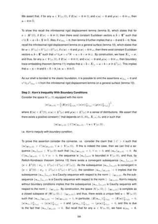
![Thus, our rigid displacement result implies that the limit is identically zero, i.e. u = 0, but this
contradicts our assumption ||um||W (ω,Ω) = 1, ∀ m > 0. This implies that our initial assumption
||u||W (ω,Ω) > C||u||S(ω,Ω), ∀ u ∈ V (ω, Ω), cannot hold, and thus, we conclude the proof by confirm-
ing that exists a positive constant C that is independent of u, such that ||u||W (ω,Ω) ≤ C||u||S(ω,Ω),
∀ u ∈ V (ω, Ω).
Our proof of Korn’s inequality is not too dissimilar to Ciarlet’s [38] proof of Korn’s inequalities for the
displacement-traction case. The only difference is that Ciarlet’s [38] Korn’s inequity for a general
surface is proved for the u|∂ω0
= 0 and nα
∂αu3
|∂ω0
= 0 case, while our Korn’s equality is proved for
the u|Ω0 = 0 case, as it was possible to omit the conditions u|∂ω0 = 0 and nα
∂αu3
|∂ω0 = 0 due to
the fact that we treated the shell as a boundary form of the foundation (please see step 2 for more
detail).
Step 4 : Zero-Slope Boundary Conditions
Now, we must show that the space VS (ω, Ω) is a proper subset of the space V (ω, Ω) that is closed
under the norm || · ||W (ω,Ω).
The rigid displacement result (see step 2) implies that for any u ∈ V (ω, Ω), if E(u) = 0 in Ω, and
(u) = 0 and ρ(u) = 0 in ω, then u = 0 in ¯Ω. Thus, if u = 0 in ¯Ω, then clearly we get (u3
|ω) = 0, in
particular ∂β(u3
|ω)|∂ω = 0, ∀ β ∈ {1, 2}. This implies that the conditions ∂β(u3
|ω)|∂ω = 0, ∀ β ∈ {1, 2}
does not violate the rigid displacement result. Thus, for any u ∈ VS (ω, Ω), we get u ∈ V (ω, Ω), i.e.
VS (ω, Ω) ⊂ V (ω, Ω).
By definition, for any v ∈ H2
(ω), we have ∂βv ∈ H1
(ω), ∀ β ∈ {1, 2}. Also, as ∂ω is a uniform-
C1
(R2
; R) boundary, trivial traces (lemma 12) implies that the space H1
0 (ω) is a proper subset of the
Hilbert space H1
(ω) that is closed under the norm || · ||H1(ω), i.e. the space (H1
0 (ω), || · ||H1(ω)) ⊂
(H1
(ω), || · ||H1(ω)) is closed. Note that for any u ∈ VS (ω, Ω), we get ∂β(u3
|ω)|∂ω = 0, ∀ β ∈ {1, 2},
and thus, we get ∂β(u3
|ω) ∈ H1
0 (ω), ∀ β ∈ {1, 2}, by trivial traces (lemma 12). Now, this implies that
the space (VS (ω, Ω), || · ||W (ω,Ω)) ⊂ (V (ω, Ω), || · ||W (ω,Ω)) is closed.
Above analyses imply that the space VS (ω, Ω) is a proper subset of the space V (ω, Ω) that is closed
under the norm ||·||W (ω,Ω). Thus, we can conclude our proof of Korn’s inequality by confirming that
||u||W (ω,Ω) ≤ C||u||S(ω,Ω), ∀ u ∈ VS (ω, Ω), where C is a positive constant that is independent of u.
3.5 Numerical Example
To conduct numerical experiments assume that one is dealing with overlying shell with a thick-
ness h that is bonded to an elastic foundation, where the unstrained configuration of the foundation
is an infinitely long annular semi-prism characterised by the diffeomorphism ¯X(x1
, x2
, x3
) = (x1
,
a sin(x2
), b cos(x2
))E+x3
(ϕ(x2
))−1
(0, b sin(x2
), a cos(x2
))E, where ϕ(x2
) = (b2
sin2
(x2
)+a2
cos2
(x2
))
1
2 ,
x1
∈ (−∞, ∞), x2
∈ (−1
2 π, 1
2 π), x3
∈ (−H, 0), and a is the horizontal radius and b is the ver-
99](https://image.slidesharecdn.com/a24f3df3-5be8-40a0-a0ff-910a71f94372-170108131508/85/PhDKJayawardana-105-320.jpg)
![tical radius of the upper surface. With some calculations, one finds that the metric tensor is
g = diag(1, ( ¯ψ2)2
, 1), where ¯ψ2 = ϕ(x2
) + x3
ab(ϕ(x2
))−2
, and Christoffel symbols are
¯Γ2
22 = ( ¯ψ2)−1
∂2
¯ψ2 ,
¯Γ2
23 = ( ¯ψ2)−1
∂3
¯ψ2 .
With few more calculations one finds
¯2u2
= ∂2u2
+ ¯Γ2
22u2
+ ¯Γ2
23u3
,
¯2u3
= ∂2u3
− ( ¯ψ2)2 ¯Γ2
23u2
,
¯3u2
= ∂3u2
+ ¯Γ2
23u2
,
¯3u3
= ∂3u3
,
where u = (0, u2
(x2
, x3
), u3
(x2
, x3
)) is the displacement field. Armed with this knowledge, one can
express the governing equations of the foundation as
(¯λ + ¯µ)∂2 ¯iui
+ ¯µ ¯∆u2
= 0 ,
(¯λ + ¯µ)∂3 ¯iui
+ ¯µ ¯∆u3
= 0 .
Now, eliminating x1
dependency one can express the remaining boundaries as
∂ΩNew
= ¯ωNew
∪ ∂ΩNew
0 ∪ ∂ΩNew
f ,
ωNew
= {(−
1
2
π,
1
2
π) × {−0}} ,
∂ΩNew
0 = {(−
1
2
π,
1
2
π) × {−H}} ,
∂ΩNew
f = {{−
1
2
π} × (−H, 0)} ∪ {{
1
2
π} × (−H, 0)} .
Thus, the boundary conditions one imposes on the foundation reduce to
u2
|∂Ω
New
0
= 0 (zero-Dirichlet) ,
u3
|∂Ω
New
0
= 0 (zero-Dirichlet) ,
( ¯ψ2)2
∂3u2
+ ∂2u3
|∂ΩNew
f
= 0 (zero-Robin) ,
(¯λ + 2¯µ)∂2u2
+ ¯λ ∂3u3
+ ¯Γ2
22u2
+ ¯Γ2
23u3
|∂ΩNew
f
= 0 (zero-Robin) .
Now, consider overlying shell’s unstrained configuration, which is described by the injective immer-
sion σ(x1
, x2
) = (x1
, a sin(x2
), b cos(x2
))E, where x1
∈ (−∞, ∞) and x2
∈ (−1
2 π, 1
2 π). With some
calculations one finds that the first fundamental form tensor is F[I] = diag(1, (ψ2)2
), the second
fundamental form tensor is F[II] = diag(0, −ab(ϕ(x2
))−1
) and only nonzero Christoffel symbol is
Γ2
22 = ψ−1
2 ∂2ψ2, where ψ2 = ϕ(x2
). With few more calculations one further finds
2u2
= ∂2u2
+ Γ2
22u2
,
2
2(u) = 2u2
− F 2
[II]2u3
,
ρ2
2(u) = ∆u3
− F 2
[II]2F 2
[II]2u3
+ 2F 2
[II]2 2u2
+ ∂2F 2
[II]2u2
,
100](https://image.slidesharecdn.com/a24f3df3-5be8-40a0-a0ff-910a71f94372-170108131508/85/PhDKJayawardana-106-320.jpg)
![where u|¯ωNew = (0, u2
(x2
, 0), u3
(x2
, 0)) is the displacement field of the shell. Thus, one may express
the governing equations of the shell as
hΛ∂2
2
2(u) +
1
3
h3
Λ(2F 2
[II]2∂2ρ2
2(u) + ∂2F 2
[II]2ρ2
2(u)) − Tr(T3
2 (u)) = 0 , (73)
−hΛF 2
[II]2
2
2(u) +
1
3
h3
Λ(∆ρ2
2(u) − F 2
[II]2F 2
[II]2ρ2
2(u)) + Tr(T3
3 (u)) = 0 , (74)
where
Tr(T3
2 (u)) = ¯µ ( ¯ψ2)2
∂3u2
+ ∂2u3
|ωNew ,
Tr(T3
3 (u)) = ¯λ ∂2u2
+ ¯Γ2
22u2
+ ¯Γ2
23u3
+ (¯λ + 2¯µ)∂3u3
|ωNew ,
and
Λ = 4µ
λ + µ
λ + 2µ
.
Now, eliminating x1
dependency one can express the remaining boundaries as
∂ωNew
= ∂ωNew
T0
∪ ∂ωNew
Tmax
,
∂ωNew
T0
= {0} ,
∂ωNew
Tmax
= {π} .
Thus, the boundary conditions of the shell reduce to
Λ 2
2(u) +
2
3
h2
ΛF 2
[II]2ρ2
2(u) |∂ωNew
T0
= τ0 (traction) ,
Λ 2
2(u) +
2
3
h2
ΛF 2
[II]2ρ2
2(u) |∂ωNew
Tmax
= τmax (traction) ,
∂2ρ2
2(u)|∂ωNew = 0 (zero-pressure) ,
∂2u3
|∂ωNew = 0 (zero-Neumann) .
Despite the fact that the original problem is three-dimensional, as a result of problem’s invariance in
the x1
direction, it is now to a two-dimensional problem. Now, the domain merely resides in the set
{(x2
, x3
) | (x2
, x3
) ∈ [−1
2 π, 1
4 π] × [−H, 0]}. Despite the fact that theorem 3 is only valid for bounded
domains, we show later that the reduced two-dimensional problem is numerically sound.
To conduct numerical experiments we use the second-order-accurate finite-difference method, but
one issue we must tackle prior is the discretisation of the (reduced two-dimensional) domain. As
we are dealing with curvilinear coordinates, there is an inherit grid dependence. To be precise, it is
approximately ψ0∆x2
≤ ∆x3
, ∀ ψ0 ∈ { ¯ψ2(x2
, x3
) | x2
∈ [−1
2 π, 1
2 π] and x3
∈ [−H, 0]}, where ∆xj
is a small increment in xj
direction. For our purposes we use ∆x2
= 1
N−1 and ψ0 = ¯ψ2(1
4 π, 0),
where N = 250 (see figure 32). We also keep the values a = 2, H = 1, ¯E = 103
, ¯ν = 1
4 , τ0 = 1
and τmax = 1 fixed for all experiments. Finally, we must define a terminating condition. For this,
we choose to terminate our iterating process once the condition |1 − ||um||−1
2 ||um+1|| 2 | < 10−10
is
satisfied, where um is the mth
iterative solution.
Figure 33 is calculated with the values b = 2, h = 1
4 , E = 6000 and ν = 1
4 . Figure 33 shows the
azimuthal (i.e. u2
) and the radial (i.e. u3
) displacements at the contact region ωNew
. The maximum
101](https://image.slidesharecdn.com/a24f3df3-5be8-40a0-a0ff-910a71f94372-170108131508/85/PhDKJayawardana-107-320.jpg)

![4.2 4.4 4.6 4.8 5 5.2 5.4 5.6
log(N)
-5.5
-5
-4.5
-4
log(Error)
Figure 34: Grid dependence of the bonded shell model.
ical solution N and N + 1 decreases. For our experiments we found that the azimuthal grid points
and the error share the relation N ∝ Error−0.851
, where Error = |1 − ||uN−1||−1
2 ||uN || 2 |. Note that
figure 33 is calculated with the values b = 2, h = 1
4 , E = 6000 and ν = 1
4 . Also, we use UCL
DPS machines (operating-system: Centos 7, CPU: 8 core Intel Xeon, memory: 64GB) to run the
numerical simulations.
While the above numerical results seem interesting, without something tangible to compare it
against any conclusions deduced from above results are merely speculative. Thus, we dedicate
the next section to numerical comparison against another, but a similar, model that is described by
the work of Baldelli and Bourdin [16].
3.6 Comparison Against the Works of Baldelli and and Bourdin
In this section we extend Baldelli and Bourdin’s [16] model for bonded films on elastic pseudo-
foundations into curvilinear coordinates. To extend Baldelli and Bourdin’s [16] model to curvilinear
coordinates consider the following: consider a thin overlying body with constant thickness h whose
unstrained configuration is described by the diffeomorphism ¯X ∈ C1
(¯ω ×(0, h); E3
), where ¯X =
(x1
, x2
, x3
) = σ(x1
, x2
) + x3
N(x1
, x2
), σ ∈ C2
(¯ω; E3
) is an injective immersion and ω ⊂ R2
is
a domain of concern, and with the displacement field of the lower-surface (w1
− x3 ¯ 1
w3, w2
−
x3 ¯ 2
w3, w3
), where w ∈ H1
(ω)×H1
(ω)×H2
(ω). Now, assume that this overlying body is bonded
to an elastic foundation with a constant thickness H whose unstrained configuration is described
by the diffeomorphism ¯X ∈ C1
(ω ×(−H, 0]; E3
) such that at x3
= −H the displacement field of
the foundation satisfies zero-Dirichlet boundary condition. Thus, in accordance with Baldelli and
Bourdin [16], we may approximate the displacement field of the foundation as u = (1 + H−1
x3
)w.
However, unlike Baldelli and Bourdin [16], we make no prior assumptions regarding the asymptotic
nature of Young’s moduli or Poisson’s ratios or the displacement fields. Now, with some asymptotic
analysis one finds that the condition {Λh ∼ H−1
¯µmeas(σ(ω); E2
), hBαβγδ
F[II]αβF[II]γδ ∼ H−1
(¯λ+2¯µ)}
103](https://image.slidesharecdn.com/a24f3df3-5be8-40a0-a0ff-910a71f94372-170108131508/85/PhDKJayawardana-109-320.jpg)
![is the only asymptotic scaling possible that yields any valid leading order solutions, i.e the scaling
that allows
h
0 ω
1
2
Bαβγδ
αβ(w1
, w2
) γδ(w1
, w2
) dωdx3
≈
0
−H ω
Aα3β3
Eα3(u1
, u2
)Eβ3(u1
, u2
) dωdx3
,
h
0 ω
1
2
Bαβγδ
αβ(w3
) γδ(w3
) dωdx3
≈
0
−H ω
1
2
A3333
E33(u3
)E33(u3
) dωdx3
.
Thus, collect all the leading order terms to find:
Corollary 3. Let ω ⊂ R2
be a connected open bounded plane that satisfies the segment
condition with a uniform-C1
(R2
; R) boundary ∂ω. Let σ ∈ C2
(¯ω; E3
) be an injective immersion.
Let f0 ∈ L2
(ω) and τ0 ∈ L2
(∂ω). If {Λh ∼ H−1
¯µmeas(σ(ω); E2
), hBαβγδ
F[II]αβF[II]γδ ∼ H−1
(¯λ +
2¯µ)}, then exists a unique field w = (w1
, w2
) ∈ H1
(ω) such that w is the solution to the
minimisation problem
J(w)Baldelli = min
v∈H1(ω)
J(v) ,
where
J(w)Baldelli =
ω
1
2
hBαβγδ M
αβ(w) M
γδ(w) +
1
2
¯µ
H
wαwα
− hfα
0 wα dω −
∂ω
hτα
0 wα d(∂ω) ,
and where Λ = 4(λ + 2µ)−1
µ(λ + µ), λ and µ are respectively first and second Lam´e’s param-
eters, h is the thickness, M
αβ(w) = 1
2 ( αwβ + βwα) is the strain tensor and B is the isotropic
elasticity tensor of the membrane, and ¯λ and ¯µ are respectively first and second Lam´e’s pa-
rameters and H is the thickness of the foundation. In particular, the unique minimiser w is
also a critical point in (H1
(ω), J(·)Baldelli).
Proof. Coersive: J(w)Baldelli ≥ C1|| M
(w)||2
L2(ω)
+ C2||w||2
L2(ω)
− C3||w||L2(ω) − C4||w||L2(∂ω) ≥
c1||w||2
H1(ω)
− c2||w||H1(ω), ∀ w ∈ H1
(ω). Note that we use the condition ||w||H1(ω) ≤
C(|| M
(w)||2
L2(ω)
+ ||w||2
L2(ω)
)
1
2 , which is Korn’s inequality without boundary conditions for
a membrane (see chapter 4 and 5 of Ciarlet [38] with w3
= 0). Fr´echet Differentiable:
J (w)Baldelliv ≤ C1|| M
(w)||L2(ω)|| M
(v)||L2(ω)+C2||w||L2(ω)||v||L2(ω)+C3||v||L2(ω)+C4||v||L2(∂ω) ≤
C(||w||H1(ω) + 1)||v||H1(ω), ∀ v, w ∈ H1
(ω). Strictly convex: (J (w)Baldelli − J (v)Baldelli)(w −
v) ≥ C1|| M
(w) − M
(v)||2
L2(ω)
+ C2||w − v||2
L2(ω)
≥ C||w − v||2
H1(ω)
, ∀ v, w ∈ H1
(ω). Thus,
lemmas 17 and 18 imply that there exists a unique field w ∈ H1
(ω) such that w is the
unique solution to the minimisation problem J(w)Baldelli = minv∈H1(ω) J(v)Baldelli. In partic-
ular, this unique minimiser w is also a critical point in (H1
(ω), J(·)Baldelli).
Alternatively, proof follows from theorem 3 in the leading order case when the foundation
takes the form Ω = ω×(−H, 0) and for the asymptotic condition {Λh ∼ H−1
¯µmeas(σ(ω); E2
),
hBαβγδ
F[II]αβF[II]γδ ∼ H−1
(¯λ + 2¯µ)}, given that the displacement field of the foundation is
approximated by u = (1 + H−1
x3
)w.
To conduct numerical experiments we remain with the framework that we introduced in Section 3.5.
Thus, given that w = (0, w2
(x2
), 0) is the displacement field of extended Baldelli and Bourdin’s
model for a membrane supported by an elastic foundation, one finds
2w2
= ∂2w2
+ Γ2
22w2
,
104](https://image.slidesharecdn.com/a24f3df3-5be8-40a0-a0ff-910a71f94372-170108131508/85/PhDKJayawardana-110-320.jpg)
![2
2(w) = 2w2
.
Thus, one can express the governing equations as
Λ∂2 (w)2
2 − ¯µ(hH)−1
(ψ2)2
w2
= 0 ,
and the boundary conditions as
Λ 2
2(w)|∂ωNew
T0
= τ0 (traction) ,
Λ 2
2(w)|∂ωNew
Tmax
= τmax (traction) .
With a little more effort, one can solve this problem explicitly. For example, given that τ0, τmax = 1,
the explicit solution is
w2
(x2
) =
sinh aαE(x2
, e)
αΛϕ(x2) cosh (aαE(e))
, (75)
where E(x2
, e) =
x2
0
(1 − e2
sin2
(θ))
1
2 dθ is the incomplete elliptic integral of the second kind,
E(e) = E(1
2 π, e) is the complete elliptic integral of the second kind, e = (1 − (b/a)2
)
1
2 is the elliptical
modulus (see chapter 17 of Abramowitz et al. [1]) and α = (¯µ/(hHΛ))
1
2 .
Let φb = (2aαE(e))2
. As a result of the asymptotic condition {hΛ ∼ H−1
¯µ(meas(σ(ωNew
); E))2
,
hB22
22F 2
[II]2F 2
[II]2 ∼ H−1
(¯λ + 2¯µ)} (modified as ω is now no longer bounded), one finds that φb ≈ 1 is
the condition that equation (75) is mostly accurate for when approximating the contact region. Thus,
we use this fact in our numerical analysis.
Now, recall equations (73) and (74), and non-dimensionalise them by substituting in the transfor-
mations (x2
, x3
) → (¯x2
, H¯x3
) and (u2
, u3
) → (¯u2
, H¯u3
). Collecting all the leading order ¯u2
terms
for the φb ≈ 1 case, and with a little intuition, one finds that the only asymptotic scaling is of signifi-
cance is aαE(x2
, e) ∼ 1
2 π, and thus, let φs = π−2
(2aαE(e))2
. This is another asymptotic scaling we
examine with the numerical experiments.
Figure 35 is calculated with the values b = 2, h = 1
4 , E = 6000 and ν = 1
4 . Figure 35 shows the
azimuthal (i.e. w2
) and the radial (i.e. w3
) displacements at the contact region ωNew
. The maximum
azimuthal displacements are observed at x2
= ±1
2 π, with respective azimuthal displacements of
w2
= ±1.43 × 10⁻⁴
. This is a significantly lower result than what is predicted by our bonded shell
model. Also, extended Baldelli and Bourdin’s model predicts the radial displacement to be identi-
cally zero, while our shell model gives nonzero radial displacement. Now, this raises an important
question: which model accurately depicts the displacement field at the contact region?
To investigate this matter further, we numerically model the overlying body as a three-dimensional
body and we do not approximate this body as a shell or otherwise. Thus, the displacement at the
contact region with this approach is the displacement field at the contact region of the bonded two-
body elastic problem, whose solution is obtained by the use of the stranded equilibrium equations
in the liner elasticity theory.
105](https://image.slidesharecdn.com/a24f3df3-5be8-40a0-a0ff-910a71f94372-170108131508/85/PhDKJayawardana-111-320.jpg)
![-2 -1.5 -1 -0.5 0 0.5 1 1.5 2
θ
-1.5
-1
-0.5
0
0.5
1
1.5
AzimuthalDisplacement
×10-4
-2 -1.5 -1 -0.5 0 0.5 1 1.5 2
θ
-1
-0.8
-0.6
-0.4
-0.2
0
0.2
0.4
0.6
0.8
1
RadialDisplacement
Figure 35: Displacement field of extended Baldelli and Bourdin’s model at the contact
region.
In accordance with the framework that is introduced in Section 3.5, the overlying body is restricted
to the region x3
∈ (0, h). Thus, with some calculations one finds
¯2v2
= ∂2v2
+ ¯Γ2
22v2
+ ¯Γ2
23v3
,
¯2v3
= ∂2v3
− ( ¯ψ2)2 ¯Γ2
23v2
,
¯3v2
= ∂3v2
+ ¯Γ2
23v2
,
¯3v3
= ∂3v3
,
where v = (0, v2
(x2
, x3
), v3
(x2
, x3
)) is the displacement field of the overlying body. With relative
ease, one can express the governing equations of the overlying body as
(λ + µ)∂2 ¯ivi
+ µ ¯∆v2
= 0 ,
(λ + µ)∂3 ¯ivi
+ µ ¯∆v3
= 0 ,
and the boundary conditions of the overlying body as
(λ + 2µ)∂2v2
+ λ ∂3v3
+ ¯Γ2
22v2
+ ¯Γ2
23v3
|{∂ωNew
T0
×[0,h]} = τ0 (traction) ,
(λ + 2µ)∂2v2
+ λ ∂3v3
+ ¯Γ2
22v2
+ ¯Γ2
23v3
|{∂ωNew
Tmax
×[0,h]} = τmax (traction) ,
λ ∂2v2
+ ¯Γ2
22v2
+ ¯Γ2
23v3
+ (λ + 2µ)∂3v3
|{(− 1
2 π, 1
2 π)×{h}} = 0 (zero-Robin) ,
( ¯ψ2)2
∂3v2
+ ∂2v3
|{∂ωNew×[0,h]}∪{(− 1
2 π, 1
2 π)×{h}} = 0 (zero-Robin) ,
with following equations characterising the bonding of the overlying body to the foundation
u2
− v2
|ωNew = 0 (continuous azimuthal displacement) ,
u3
− v3
|ωNew = 0 (continuous radial displacement) ,
Tr(T2
3 (u)) − µ ( ¯ψ2)2
∂3v2
+ ∂2v3
|ωNew = 0 (continuous azimuthal stress) ,
Tr(T3
3 (u)) − λ ∂2v2
+ ¯Γ2
22v2
+ ¯Γ2
23v3
+ (λ + 2µ)∂3v3
|ωNew = 0 (continuous radial stress) .
106](https://image.slidesharecdn.com/a24f3df3-5be8-40a0-a0ff-910a71f94372-170108131508/85/PhDKJayawardana-112-320.jpg)
![-2 -1.5 -1 -0.5 0 0.5 1 1.5 2
y-axis
-0.5
0
0.5
1
1.5
2
2.5
z-axis
Overlying Body
Foundation
Figure 36: Discretised reduced two-dimensional domain of the two-body elastic problem
for the a = 2, b = 2, h = 1
8 , H = 1 and N = 250 case.
Note that the grid dependence of the overlying body is approximately ψ0∆x2
≤ ∆x3
, ∀ ψ0 ∈
{ ¯ψ2(x2
, x3
) | x2
∈ [−1
2 π, 1
2 π] and x3
∈ [0, h]}, where ∆xj
is a small increment in xj
direction. For our
purposes, we use ∆x2
= 1
N−1 and ψ0 = ¯ψ2(1
4 π, h), where N = 250 (see figure 36). Furthermore, we
choose to terminate our iterating process once the condition |1−(||um|| 2 +||vm|| 2 )−1
(||um+1|| 2 +
||vm+1|| 2 )| < 10−10
is satisfied, where um and vm are the mth
iterative solutions of the bonded
two-body model.
-2 -1.5 -1 -0.5 0 0.5 1 1.5 2
θ
-3
-2
-1
0
1
2
3
AzimuthalDisplacement
×10-4
-2 -1.5 -1 -0.5 0 0.5 1 1.5 2
θ
-3.5
-3
-2.5
-2
-1.5
-1
RadialDisplacement
×10-4
Figure 37: Displacement field of the bonded two-body model at the contact region.
107](https://image.slidesharecdn.com/a24f3df3-5be8-40a0-a0ff-910a71f94372-170108131508/85/PhDKJayawardana-113-320.jpg)
![Figure 37 is calculated with the values of b = 2, h = 1
4 , E = 6000 and ν = 1
4 . Figure 37 shows the
azimuthal (i.e. v2
) and the radial (i.e. v3
) displacements at the contact region ωNew
. The maximum
azimuthal displacements are observed at x2
= ±1
2 π, with respective azimuthal displacements of
v2
= ±2.78 × 10⁻⁴
. The maximum radial displacement is observed at x2
= ±1
2 π, with a radial dis-
placement of v3
= −3.24 × 10⁻⁴
. This implies that our overlying shell model’s prediction is closer to
bonded two-body’s displacement field at the contact region relative to extended Baldelli and Bour-
din’s model’s prediction, for this case of course.
4.2 4.4 4.6 4.8 5 5.2 5.4 5.6
log(N)
-5.5
-5
-4.5
-4
log(Error)
Figure 38: Grid dependence of the bonded two-body model.
As for the analysis on grid dependence, the reader can see from figure 38, as N increases,
the difference between the numerical solution N and N + 1 decreases. For our experiments
we found that the azimuthal grid points and the error share the relation N ∝ Error−0.894
, where
Error = |1 − (||uN−1|| 2 + ||vN−1|| 2 )−1
(||uN || 2 + ||vN || 2 )|. Note that figure 37 is calculated with
the values of b = 2, h = 1
4 , E = 6000 and ν = 1
4 .
But this is still not sufficient analysis, and thus, our goal in this section is to investigate how our
bonded shell model approximates bonded two-body model’s displacement field at the contact region
relative to extended Baldelli and Bourdin’s model for the variables δb = b/a, δh = h/H, δE = E/ ¯E
and δν = ν/¯ν. To proceed with this investigation we calculate the error in the energy-norm (see
Jayawardana et al. [89]) as
Err2(ui
) =
{∆x2} ||ui
shell(∆x2
, 0) − ui
two-body(∆x2
, 0)||2
1
2
{∆x2} ||ui
two-body(∆x2, 0)||2
1
2
,
Err2(wi
) =
{∆x2} ||wi
Baldelli(∆x2
) − ui
two-body(∆x2
, 0)||2
1
2
{∆x2} ||ui
two-body(∆x2, 0)||2
1
2
,
to calculate the relative error between the bonded two-body displacement field and the approxi-
mated displacement fields at the contact region.
108](https://image.slidesharecdn.com/a24f3df3-5be8-40a0-a0ff-910a71f94372-170108131508/85/PhDKJayawardana-114-320.jpg)
![0 0.1 0.2 0.3 0.4 0.5
δh
0
0.1
0.2
0.3
0.4
0.5
0.6
AzimuthalErr2
Baldelli
Shell
0 0.1 0.2 0.3 0.4 0.5
δh
0
0.1
0.2
0.3
0.4
0.5
0.6
0.7
0.8
0.9
1
RadialErr2
Baldelli
Shell
Figure 39: Shell model error v extended Baldelli and Bourdin’s model error for δh = h/H.
Figure 39 is calculated with the values δb = 1, δh ∈ { 1
20 , 2
20 , 3
20 , 4
20 , 5
20 , 6
20 , 7
20 , 8
20 , 9
20 , 10
20 }, δE = 6 and
δν = 1. From figure 39 one can see that the azimuthal error of the extended Baldelli and Bourdin’s
model attains a minimum at δh = 3
20 with an azimuthal error of 50.4%. This coincides with the
asymptotic condition φb, as when φb ≈ 1, one observes this minimum in the azimuthal error. Notice
how extended Baldelli and Bourdin’s azimuthal error increases as the thickness of the overlying
body decreases. Now, this raises an important issue regarding Baldelli and Bourdin’s work [16] as
the authors present their model to be valid for analysing overlying thin objects, yet the asymptotic
condition φb implies that their assertion cannot be valid, i.e. authors’ model is mostly accurate for
overlying bodies with a very specific thickness. Now, consider the azimuthal error of our bonded
shell model, and it is significantly smaller than the error of extended Baldelli and Bourdin’s model.
For our bonded shell model the maximum azimuthal error is observed at δh = 1
4 with an error of
3.32%, and it rapidly decreases as δh decreases or increases. This maximum in azimuthal error of
the bonded shell model is observed for the asymptotic condition φs = 1. The radial error of extended
Baldelli and Bourdin’s model is 100% and this is the case for all values of δh. This is due to the fact
that with extended Baldelli and Bourdin’s model the only value the normal displacement can obtain
is zero, and this is case for all variables. In contrast, the radial error of our bonded shell model
is, again, significantly smaller. For the shell model, the highest radial error is, again, observed at
δh = 1
4 , with an error of 12.9%. This maximum in radial error of the shell model is observed again
for the asymptotic condition φs = 1.
Figure 40 is calculated with the values δb = 1, δh = 1
4 , δE ∈ {1, 2, 3, 4, 5, 6, 7, 8, 9, 10} and δν = 1.
From figure 40 one can see that the azimuthal error of extended Baldelli and Bourdin’s model attains
a minimum at δE = 4 with an azimuthal error of 50.8%. This, again, coincides with the asymptotic
condition φb, as when φb ≈ 1, we observe this minimum in the azimuthal error. Notice how ex-
tended Baldelli and Bourdin’s azimuthal error increases as Young’s modulus of the overlying body
increases. Now, this raises an important issue regarding Baldelli and Bourdin’s work [16] as the au-
109](https://image.slidesharecdn.com/a24f3df3-5be8-40a0-a0ff-910a71f94372-170108131508/85/PhDKJayawardana-115-320.jpg)
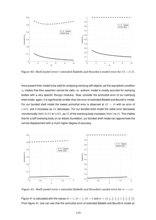
![tains a minimum at δν = 0, with an azimuthal error of 50.4%. This, once again, coincides with the
asymptotic condition φb, as when φb ≈ 1, we observe this minimum in the azimuthal error. Now, this
raises an important issue regarding Baldelli and Bourdin’s work [16] as the authors present their
model to be valid for overlying bodies with nonzero Poisson’s ratios, yet the asymptotic condition
φb implies that their assertion cannot be valid, i.e. authors’ model is mostly accurate for overlying
bodies with zero-Poisson’s ratio. Now, consider azimuthal error from our bonded shell model, it is,
again, significantly smaller than the error of extended Baldelli and Bourdin’s model. For our bonded
shell model the highest azimuthal error is observed at δν = 8
5 with an error of 3.56%. Also, for
our bonded shell model the radial error increases monotonically, from 11.6% to 14.2%, as δν of the
overlying body increases, from 0 to 9
5 .
0.7 0.8 0.9 1 1.1 1.2 1.3
δb
0
0.1
0.2
0.3
0.4
0.5
0.6
0.7
AzimuthalErr2
Baldelli
Shell
0.7 0.8 0.9 1 1.1 1.2 1.3
δb
0
0.1
0.2
0.3
0.4
0.5
0.6
0.7
0.8
0.9
1
RadialErr2
Baldelli
Shell
Figure 42: Shell model error v extended Baldelli and Bourdin’s model error for δb = b/a.
Figure 42 and calculated with the values δb ∈ {15
20 , 16
20 , 17
20 , 18
20 , 19
20 , 1, 21
20 , 22
20 , 23
20 , 24
20 , 25
20 }, δh = 1
4 , δE = 6
and δν = 1. From figure 42, one can see that the azimuthal error of extended Baldelli and Bourdin’s
model decreases monotonically with increasing δb, and at δb = 5
4 , the azimuthal error is 46.3%.
This, however, is not predicted by the asymptotic condition φb as in accordance with the condition
φb ≈ 1 we expect to observe this minimum in the azimuthal error at δb = 1 i.e. when the mean
curvature of the system is constant. Now, consider the azimuthal error of our bonded shell model,
once more, it is significantly smaller than the error of extended Baldelli and Bourdin’s model. The
lowest azimuthal error of our bonded shell model is observed at δb = 17
20 with an error of 1.02% and
this error increases as δb increases or decreases. These results imply that there exists a critical
parametric-latitude where the azimuthal error of our shell model is a minimum. For the bonded shell
model the radial error increases monotonically, from 3.78% to 18.9% as δb increases, from 3
4 to 5
4 .
The above analysis appears show that our bonded shell on an elastic foundation model is far su-
perior to extended Baldelli and Bourdin’s model with respect to the bonded two-body model, as
extended Baldelli and Bourdin’s model’s error failed to fall below or even come close to our bonded
shell model’s error, even a for set of variables which extended Baldelli and Bourdin’s model is mostly
111](https://image.slidesharecdn.com/a24f3df3-5be8-40a0-a0ff-910a71f94372-170108131508/85/PhDKJayawardana-117-320.jpg)
![accurate for. Also, extended Baldelli and Bourdin’s model asserts that the normal displacement is
always zero, while our bonded shell model can predict a nonzero normal displacement, often dif-
fering from two-body problem’s solution by 10%. Another disadvantage of extended Baldelli and
Bourdin’s model is that, for the model to be valid, the foundation must have a very specific form (i.e.
constant thickness H, planer dimension cannot exceed the contact region ω, the lower boundary
must satisfy zero-Dirichlet boundary condition and the remaining boundaries must be stress free),
while for our bonded shell model the foundation may take arbitrary form, as long as in a proper sub-
set of the boundary of the foundation the displacement field of the foundation satisfies zero-Dirichlet
boundary condition. However, there are some advantages of extended Baldelli and Bourdin’s model
over our bonded shell model. For example, extended Baldelli and Bourdin’s model is extremely sim-
ple to numerically model as it approximates the foundation. Thus, often a closed-form of a solution
can be found, while our bonded shell model requires lengthy computations to calculate solutions,
even for a simple problem such as the one investigated in this section.
The numerical results raise fundamental questions regarding extended Baldelli and Bourdin’s model.
As δh decreases beyond a certain threshold, extended Baldelli and Bourdin’s solution diverge away
from two-body model’s azimuthal solution, implying that extended Baldelli and Bourdin’s model is
mostly accurate for overlying bodies with a very specific thickness. However, Baldelli and Bourdin
[16] assert that their model is to be used for overlying thin bodies, such as thin films and membranes.
Clearly our numerical experiments (see figure 39) contradict their assertion about the model must
be used for modelling very thin overlying bodies. Another peculiar behaviour we observed is that
as δE of the overlying body increases above a certain threshold, extended Baldelli and Bourdin’s
azimuthal error diverge away from two-body model’s azimuthal solution. This, again, contradicts
authors’ asymptotic assertion, which states that the stiffer the overlying body is, then more accurate
their model is. Furthermore, we observed that then the Poisson’s ratio of the overlying body is zero
Baldelli and Bourdin’s azimuthal error attains a minimum. This, further, contradicts authors’ asymp-
totic assertion, which states that the Poisson’s ratio of the overlying body must be sufficiently away
from zero for the model to be mostly accurate. Note that we do not find any numerical evidence in
authors’ publications (or Baldelli [15]) to support theirs asymptotic assertions.
On a last note: we remind the reader again that the model we present in this section is not a
model derived by Baldelli and Bourdin [16]. We merely called it the extended Baldelli and Bourdin’s
model for convenience. The main thing we used from the authors is that their approximate for the
displacement field of the foundation, which is u = (1 + H−1
x3
)w where w is the displacement filed
of the overlying body at the contact region. Please see Section 1.10 for a comprehensive review of
authors’ work.
3.7 Error analysis
It is documented in the literature that given a thin overlying body on an elastic foundation, the thin
body must only be approximated by a shell (a plate, a membrane or a film), if the thin overlying body
112](https://image.slidesharecdn.com/a24f3df3-5be8-40a0-a0ff-910a71f94372-170108131508/85/PhDKJayawardana-118-320.jpg)
![has a significantly higher Young’s modulus relative to Young’s modulus of the foundation[4]. In light
of this information we dedicate this section to see how physically valid our bonded shell model is
with respect to varying elastic and geometrical properties.
To proceed with this investigation we calculate the relative error between the displacement field of
the foundation predicted by our bonded shell model and the displacement field of the foundation
predicted by the bonded two-body elastic model by
Relative Error(ui
) =
{∆x2,∆x3} ||ui
shell(∆x2
, ∆x3
) − ui
two-body(∆x2
, ∆x3
)||2
1
2
{∆x2,∆x3} ||ui
shell(∆x2, ∆x3) + ui
two-body(∆x2, ∆x3)||2
1
2
.
We retain the same numerical procedure that we introduced in Sections 3.5 and 3.6, and see how
the relative error behaves for various values of δE = E/ ¯E, δν = ν/¯ν, δh = h/H, and δb = b/a.
0 2 4 6 8 10 12 14 16
δE
0.005
0.01
0.015
0.02
0.025
0.03
0.035
0.04
AzimuthalRelativeError
0 2 4 6 8 10 12 14 16
δE
0.02
0.03
0.04
0.05
0.06
0.07
0.08
RadialRelativeError
Figure 43: Relative error for δE = E/ ¯E.
Figure 43 is calculated with the values δb = 1, δh = 1
8 , δE ∈ {1, 3
2 , 2, 5
2 , 3, 7
2 , 4, 9
2 , 5, 11
2 , 6, 13
2 , 7, 15
2 , 8,
17
2 , 9, 19
2 , 10, 21
2 , 11, 22
2 , 12, 25
2 , 13, 27
2 , 14, 29
2 , 15, 31
2 , 16} and δν = 1. From figure 43 one can see that
the azimuthal relative error attains a minimum at δE = 13
2 with a relative error of 0.852%. Now, this
implies that, despite the fact that a higher Young’s modulus of the shell results in more accurate
solutions, increasing Young’s modulus of the shell indefinitely may not result in the most accurate
solutions. We observe a similar effect in Section 3.6, where the model presented assumed to
be valid for membranes with high Young’s moduli, yet we observed that there exists an optimum
Young’s modulus where the error is a minimum. As for the relative radial error, one can see that
as δE of shell increases, from 1 to 16, the relative error decreases, from 7.59% to 2.74%. Now, to
reduce the radial error, it appears to be a sound choice to increase Young’s modulus of the shell to
extremely high values.
Figure 44 is calculated with the values δb = 1, δh ∈ { 2
32 , 3
32 , 4
32 , 5
32 , 6
32 , 7
32 , 8
32 , 9
32 , 10
32 , 11
32 , 12
32 }, δE = 8
and δν = 1. From figure 44 one can see that the azimuthal relative error attains a minimum at
113](https://image.slidesharecdn.com/a24f3df3-5be8-40a0-a0ff-910a71f94372-170108131508/85/PhDKJayawardana-119-320.jpg)
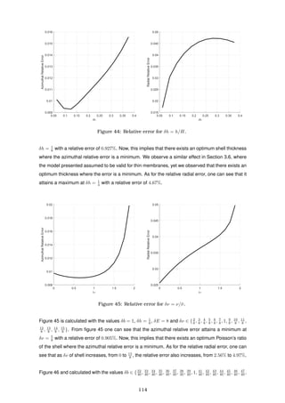
![0.8 0.85 0.9 0.95 1 1.05 1.1 1.15 1.2
δb
0.009
0.0095
0.01
0.0105
0.011
0.0115
0.012
0.0125
0.013
0.0135
0.014
AzimuthalRelativeError
0.8 0.85 0.9 0.95 1 1.05 1.1 1.15 1.2
δb
0.015
0.02
0.025
0.03
0.035
0.04
0.045
0.05
RadialRelativeError
Figure 46: Relative error for δb = b/a.
48
40 }, δh = 1
8 , δE = 8 and δν = 1. From figure 46, one can see that the azimuthal relative error at-
tains a minimum at δb = 39
40 with a relative error of 0.920%. Now, this implies that when the mean
curvature of the contact region is almost constant, the azimuthal relative error attains a minimum.
As for the relative radial error, one can see that as δb increases, from 4
5 to 6
5 , the relative error
increases, from 1.72% to 4.96%.
Above analyses show that our bonded shell on an elastic foundation can predict the displacement
field of foundation of the bonded two-body elastic model, with a significant degree of accuracy,
given that Young’s modulus of the shell is significantly high. Now, this result coincides with what
is documented in the literature [4]. However, we also observe that arbitrary increasing Young’s
modulus of the shell may not result in the most accurate solutions as for the azimuthal relative er-
ror, we observed an optimum Young’s modulus where the error is a minimum. We also observe
that other factors can equally improve the accuracy of our bonded shell model, such as the mag-
nitude of Poisson’s ratio of the shell, the thickness of the shell and the critical parametric-latitude
of the contact region, i.e. all elastic properties and geometric properties affect the accuracy of the
solution. However, one cannot arbitrarily increase or decrease the thickness, Poisson’s ratio or
critical parametric-latitude, as we often observe optimal values for elastic and geometric properties
where the error is a minimum. To to obtain the exact conditions where our bonded shell model is
asymptotically justifiable require further analysis.
3.8 Conclusions
In this chapter we studied bonded shells on elastic foundations. In Section 3.2 we derived a math-
ematical model for a bonded shell on an elastic foundation, by modifying Koiter’s linear shell equa-
tions presented by Ciarlet [38] and by considering a similar logical process that is used in the
derivation of surface Cauchy-Bourne model [89], to describe the behaviour of a shell if it is bonded
to a three-dimensional elastic body, by treating the shell as a boundary form of the foundation,
115](https://image.slidesharecdn.com/a24f3df3-5be8-40a0-a0ff-910a71f94372-170108131508/85/PhDKJayawardana-121-320.jpg)
![which is analogous to the work of Necas et al. [144]. Then, in Section 3.3, we explicitly derived the
governing equations and the boundary conditions for the general case for bonded shells on elastic
foundations. In Section 3.4 we used a combination of Ciarlet’s [38], and Badiale and Serra’s [13]
work to prove the existence and the uniqueness of the solutions, and thus, proving that what we
derived is a mathematical theory and not a hypothetical model.
In Section 3.5 we presented framework to conduct a set of numerical solutions. As a comparison,
in Section 3.6, we extended Baldelli and Bourdin’s [16] model for bonded films on elastic pseudo-
foundations to curvilinear coordinates and showed how numerical solutions fair against our bonded
shell model. The method of numerical analysis is simple: we numerically model the bonded two-
body problem and compare the solution against our bonded shell model and extended Baldelli and
Bourdin’s model, for a set of variables which extended Baldelli and Bourdin’s model is mostly accu-
rate for, i.e. for φb ≈ 1. The numerical solutions shows that our bonded shell model is far superior
when it comes to approximating displacement filed at the contact region than extended Baldelli and
Bourdin’s model, as often our azimuthal shell solution only differs from bonded two-body model’s
solution by 1−5%, while extended Baldelli and Bourdin’s azimuthal solution can differ from the from
bonded two-body model’s solution by 50%. For an extreme example, for the case δh = 1
20 we see
that the azimuthal error of the shell solution is 0.998%, while azimuthal error of extended Baldelli and
Bourdin’s solution is 51.5% (see figure 39). Also, extended Baldelli and Bourdin’s model assumes
that the normal displacement is always zero, while our shell model predicts a normal displacement
closer to the bonded two-body model’s normal displacement, often with 10% difference.
We also saw that the asymptotic scaling φb is a great indicator for judging how accurate extended
Baldelli and Bourdin’s model is, as for a given thickness, Young’s modulus, Poisson’s ratio of the
overlying body, the condition φb ≈ 1 yield the solutions with the minimum error. However, the scaling
φb failed to predict the validity of the solution with respect to the critical parametric-latitude of the
contact region. In contrast, we observe that the asymptotic scaling φs is a good indicator of judging
how invalid our bonded shell model is for a given thickness, as for a given δh, the condition φs = 1
yield the solutions with the maximum error. However, even for this case our shell model solution is
still several magnitudes closer to the bonded two-body solution than extended Baldelli and Bour-
din’s solution (see figure 39).
To conclude our numerical analysis, in Section 3.7, we conducted further error analysis to see how
our bonded shell on an elastic foundation can approximate the displacement field of the foundation
of the two-body elastic model. Our analyses how that our bonded shell model can approximate the
displacement field of foundation with a significant degree of accuracy given that Young’s modulus
of the shell is significantly high. Now, this result coincides with what is documented in the literature
[4]. We further the found that, if the thickness the shell, Poisson’s ratio of the shell and the critical
parametric-latitude of the contact region are very low, then the relative error is very small. However,
one cannot arbitrarily increase Young’s modulus of the shell or decrease the thickness the shell,
Poisson’s ratio of the shell and the critical parametric-latitude of the contact region, as we often
116](https://image.slidesharecdn.com/a24f3df3-5be8-40a0-a0ff-910a71f94372-170108131508/85/PhDKJayawardana-122-320.jpg)
![observe optimal values for elastic and geometric properties where the relative error is a minimum.
With our analyses we shown that our theory for bonded shells on elastic foundations is mathemati-
cally valid via the existence of unique solutions, numerically superior to an existing model that model
the same problem, and under which elastic and geometrical properties can one obtains the most
accurate solutions. These types of models are largely used in the field of flexible and stretchable
electronics. The reader can find a rich literature review regarding this subject matter in Section 1.7.
For example, consider a curved flexible display screen. One may model the flexible organic layer
as an elastic foundation and the thin conductive layer as a thin shell. Thus, by using our theory
for bonded shells on elastic foundations, one may derive an accurate depiction of the displacement
field and the stress profiles for the body in question, with respect to an appropriate set of variables.
3.8.1 Remark
Cortical plate
Subplate
White matter zone y
GW 22
GW 40
GW 29
GW 34
Adult
GW 26
Simulation mesh from
MRI image
at GW 22
Tangential
expansion
Figure 47: ‘A simulation starting from a smooth fetal brain shows gyrification as a result
of uniform tangential expansion of the cortical layer. The brain is modelled as a soft elastic
solid and a relative tangential expansion is imposed on the cortical layer as shows at left,
and the system allowed to relax to its elastic equilibrium’ [192].
A further possible area of application for our theory for bonded shells on elastic foundations can be
in modelling gyrification. Gyrification is the formation of folds in the cerebral cortex during the devel-
opment of the brain. Tallinen et al. [191] numerically shows that gyrification is the result of mechan-
ical buckling of the cortical plate due to rapid tangential expansion of gray matter zone constrained
by the white matter zone (see figure 47). The authors model the human brain as a thin elastic
body that is bonded to a thicker elastic body (spherical and ellipsoidal for the three-dimensional
case) with zero-Dirichlet boundary condition imposed on the lowest of its boundary (see figure 48).
The thin elastic body is assumed to be only 10% of the thickness of the elastic foundation. Both
two-dimensional and three-dimensional numerical solutions are constructed with the finite-element
method with an explicit solver for quasistatic equilibration of the system. Two-dimensional solutions
are based on constant strain triangle with 60 layers of elements through its thickness to model the
cortical plate, and three-dimensional solutions are based on irregular tetrahedron or curved cube
mesh (for large brain simulations) with 8 layers of elements through its thickness to model the corti-
cal plate.
117](https://image.slidesharecdn.com/a24f3df3-5be8-40a0-a0ff-910a71f94372-170108131508/85/PhDKJayawardana-123-320.jpg)
![Figure 48: ‘Cross-section views of 3D simulation geometries for small and large brains in
their initial undeformed states. The gray-matter thickness T, brain radius R, and bound-
ary conditions are indicated. A detailed image of the regular mesh structure of the large
brain domain shows the reflection symmetry between every pair of elementary cubes that
share a face’ [191].
A word of caution: Tallinen et al. [191] referrer to the overlying elastic layer as a shell, but it is not a
shell in the sense of mathematical shells as we investigate here in this thesis.
But what if such a fine mesh is not possible due to computational restraints or what if one wishes to
model brain with a high gyrencephalic index where the gray matter layer is significantly thinner than
white matter zone, i.e. the brains of Cetaceans (whales and dolphins) [198, 133]. For such scenar-
ios we propose that one may use our theory for bonded shells on elastic foundations. This proposal
is further justified, considering that Tallinen et al.’s [191] model (see figure 48) is schematically iden-
tical to the numerical model that we analysed in this chapter (see figure 36) with the exceptions of
that Tallinen et al. [191] did not approximate the thin layer, they are considering quasistatic case and
they are using finite strains. For more on nonlinear elasticity and the dynamic case please consult
chapter 5.
118](https://image.slidesharecdn.com/a24f3df3-5be8-40a0-a0ff-910a71f94372-170108131508/85/PhDKJayawardana-124-320.jpg)
![4 Shells Supported by Elastic Foundations: Constraints
to Model the Frictionally Coupled Case
Abstract
In this chapter we derive a theory for frictionally coupled shells on elastic foundations. We
show that, if the diffeomorphism ¯X ∈ C2
(¯Ω; E3
) describes the unstrained configuration of the
foundation and the injective immersion σ ∈ C3
(¯ω; E3
) describes the unstrained configuration of
the overlying frictionally coupled shell, where Ω ⊂ R3
is a connected open bounded domain that
satisfies the segment condition with a uniform-C1
(R3
; R2
) boundary ∂Ω such that ω, ∂Ω0 ⊂ ∂Ω,
¯ω ∩ ¯∂Ω0 = Ø, meas(∂Ω0; R2
) > 0, and ω ⊂ R2
is a connected open bounded plane that satisfies
the segment condition with a uniform-C1
(R2
; R) boundary ∂ω, with f ∈ L2
(Ω), f0 ∈ L2
(ω) and
τ0 ∈ L2
(∂ω), then there exists a unique field u ∈ VF (ω, Ω) such that u is the solution to the
minimisation problem
J(u) = min
v∈VF (ω,Ω)
J(v) ,
where
VF (ω, Ω) = {v ∈ VS (ω, Ω) | 2νF v3
+ (vαvα
)
1
2 |ω ≤ 0 a.e.} ,
J(u) =
Ω
1
2
Aijkl
Eij(u)Ekl(u) − fi
ui dΩ
+
ω
1
2
Bαβγδ
h αβ(u) γδ(u) +
1
3
h3
ραβ(u)ργδ(u) − hfi
0ui dω −
∂ω
hτi
0 ui d(∂ω) ,
and where A is the elasticity tensor and E(·) is the stain tensor of the foundation, B is the
elasticity tensor, (·) is half of the change in first fundamental form tensor, ρ(·) is the change in
second fundamental form tensor and h is the thickness of the shell, and νF is the coefficient of
friction between the foundation and the shell.
4.1 Introduction
In this chapter we examine the behaviour of shells supported by elastic foundations when subjected
to a friction condition. In Section 4.2 we use Kikuchi and Oden’s [102] model for Coulomb’s law of
static friction to derive a displacement-based static friction condition. Then, we take the overlying
shell theory that we derived in chapter 3, but now, we assert that the shell is no longer bonded to
the foundation and we use the displacement-based friction condition to transform the model into a
constrained type problem. Then, in Section 4.3, we explicitly derive the governing equations and the
boundary condition for the general case. In Section 4.4 we prove the existence and the uniqueness
of solutions of the derived model, and conclusively proving what we derived is a mathematical
theory. In Section 4.5 we present numerical examples to examine the properties for the given
theory. Then, in Section 4.6, we extend Kikuchi and Oden’s model for Coulomb’s law of static
friction in the curvilinear space that we derived in Section 2.6 to model a two-body contact problem,
i.e. an elastic two-body contact problem subjected to Coulomb’s law of static friction in curvilinear
coordinates. We use this extended Kikuchi and Oden’s model to numerically simulate an overlying
thin, but still three-dimensional, body on an elastic foundation and compare the results with our shell
model with friction to see how the both models predict the displacement field of the foundation, for
a given set of variables.
119](https://image.slidesharecdn.com/a24f3df3-5be8-40a0-a0ff-910a71f94372-170108131508/85/PhDKJayawardana-125-320.jpg)
![4.2 Derivation
Recall Kikuchi and Oden’s model for Coulomb’s law of static friction that we extended to curvilinear
coordinates, i.e. equation (66). By eliminating the regularisation parameter, ε, from the equations
one may express it in the following form,
Tβ
3 (u) + νF (g33)
1
2
(uαuα
)− 1
2 T3
3 (u)uβ
≤ 0 .
Now, assume that uβ
≥ 0 and contract the above equation with uβ
. Noting that in this framework
g33 = 1, and thus, one finds
µ uα ¯αu3
+
1
2
¯3(uαuα
) + νF (uαuα
)
1
2 λ ¯αuα
+ (λ + 2µ) ¯3u3
≤ 0 .
Now, assume that this body is in contact with an elastic foundation, and thus, it permits normal
displacements at the contact region, so assume that only the normal derivatives are of any conse-
quence. Thus, one may approximate the above relation as
µ ¯3(uαuα
)
1
2 + νF (λ + 2µ) ¯3u3
≤ 0 .
To simplify the matters further assume that the above condition is independent of any elastic prop-
erties of the overlying body. This may be achieved by assuming λ = 0, and thus, one finds
¯3 (uαuα
)
1
2 + 2νF u3
≤ 0 .
By approximating the above condition even further we arrive at the third hypothesis of our thesis:
Hypothesis 3. A shell supported by an elastic foundation with a rough contact area that is
compliant with assertion 1 satisfies the following displacement-based friction condition
u3
≤ −
1
2νF
(uαuα
)
1
2 ,
where νF is the coefficient of friction between the shell and the foundation, and u is the
displacement field of the shell with respect to the contact region. If 2νF u3
+(uαuα
)
1
2 < 0, then
we say that the shell is bonded to the foundation, and, if 2νF u3
+ (uαuα
)
1
2 = 0, then we say
that the shell is at limiting equilibrium.
The justifications for introducing the hypothesis 3 is as follows. Recall equation (42): which asserts
that the variational form of a linear elastic body subjected to Coulomb’s law of static friction is non-
convex and non-differentiable. Thus, the existence of a (unique or otherwise) solution is an open
question that cannot be proven with conventional means. But, we show that the variational form, i.e.
the energy functional of a linear elastic body subjected to the displacement-based friction condition
from hypothesis 3, is convex, coercive and differentiable, and thus, proving the existence of solu-
tions is perfectly possible. Also, unlike Kikuchi and Oden’s [102] model, hypothesis 3 is independent
of the regularisation parameter, ε, and it is well defined for all finite values of u. Furthermore, we
show that our problem can be numerically modelled without an initial guess of the purely normal
stress, which is something Kikuchi and Oden’s [102] model is incapable of. Note that we can guar-
antee that the condition from hypothesis 3 holds as we already asserted that the lower-surface of
the shell is not hyperbolic and it is a surface of positive mean curvature (see assertion 1). Thus, for
120](https://image.slidesharecdn.com/a24f3df3-5be8-40a0-a0ff-910a71f94372-170108131508/85/PhDKJayawardana-126-320.jpg)
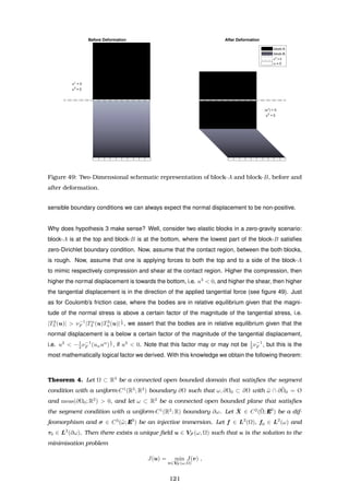
![where
VF (ω, Ω) = {v ∈ VS (ω, Ω) | 2νF v3
+ (vαvα
)
1
2 |ω ≤ 0 a.e.} ,
J(u) =
Ω
1
2
Aijkl
Eij(u)Ekl(u) − fi
ui dΩ
+
ω
1
2
Bαβγδ
h αβ(u) γδ(u) +
1
3
h3
ραβ(u)ργδ(u) − hfi
0ui dω −
∂ω
hτi
0 ui d(∂ω) ,
and νF is the coefficient of friction between the foundation and the shell.
Proof. See Section 4.4.
What does theorem 4 mean? Well, it means that given some well-posed normal and tangential
forcings, and tractions acting on a shell with a thickness h that is frictionally coupled to an elastic
foundation has a unique weak solution. This weak solution is sufficient for finding finite-element
solutions. However, due to the constraint [2νF u3
+ (uαuα
)
1
2 ]|ω ≤ 0 a.e. the unique minimiser u may
fail be a critical point in (VF (ω, Ω), J(·)). Thus, to model finite-element solutions competently one
requires the following:
Corollary 4. Let u ∈ VF (ω, Ω) be the unique solution to the minimisation problem J(u) =
minv∈VF (ω,Ω) J(v), then we get the following variational inequity
0 ≤ J (u)(v − u) , ∀ v ∈ VF (ω, Ω) .
Proof. As (VF (ω, Ω), J(·)) is a convex space (see Section 4.4), for any u, v ∈ VF (ω, Ω) we have
(1 − t)u + tv ∈ VF (ω, Ω), ∀ t ∈ [0, 1] (see definition 19). Now, let u be the unique minimiser,
then we have relation J(u) ≤ J((1−t)u+tv), ∀ t ∈ [0, 1]. This implies that, as a function of t,
J((1−t)u+tv) has a global minimum at t = 0 in the set [0, 1]. As J(·) is a convex functional
in the set VF (ω, Ω), we get ∂tJ((1 − t)u + tv)|t=0 ≥ 0, i.e. 0 ≤ J (u)(v − u), ∀ v ∈ VF (ω, Ω). See
section 8.4.2 of Evans [63] for the original proof.
For a comprehensive study of finite-element modelling of similar problems, please consult chapter
4 of Kikuchi and Oden [102]. Also, one requires higher regularity results to prove the existence of
classical solutions. This problem is a subject of discussion in Section 5.3.
4.3 Equations of Equilibrium
For this section we assume that u ∈ C2
(Ω; R3
), uα
|ω ∈ C3
(ω), u3
|ω ∈ C4
(ω) and 2νF u3
+(uαuα
)
1
2 ≤
0 everywhere in ω, and we use theorem 4 and corollary 4 to derive a set of governing equations
and boundary conditions to our problem.
4.3.1 Governing Equations of the Elastic Foundation
¯iTi
j (u) + fj = 0 , ∀ j ∈ {1, 2, 3} ,
where Tij
(u) = Aijkl
Ekl(u) is second Piola-Kirchhoff stress tensor, Eij(u) = 1
2 (gik
¯juk
+gjk
¯iuk
)
is linearised Green-St Venant stress tensor, Aijkl
= ¯λgij
gkl
+ ¯µ(gik
gjl
+ gil
gjk
) is the isotropic
122](https://image.slidesharecdn.com/a24f3df3-5be8-40a0-a0ff-910a71f94372-170108131508/85/PhDKJayawardana-128-320.jpg)
![elasticity tensor, ¯λ = (1 − ¯ν − 2¯ν2
)−1
¯ν ¯E is first Lam´e’s parameter, ¯µ = 1
2 (1 + ¯ν)−1 ¯E is second
Lam´e’s parameter, ¯E is Young’s modulus and ¯ν is Poisson’s ratio of the elastic foundation and f is
an external force density field acting on the elastic foundation.
4.3.2 Boundary Conditions of the Elastic Foundation
u|∂Ω0 = 0 ,
¯niTi
j (u)|{∂Ω{ω∪∂Ω0}} = 0 , ∀ j ∈ {1, 2, 3} ,
where ¯n is the unit outward normal to the boundary ∂Ω in curvilinear coordinates.
4.3.3 Governing Equations of the Overlying Shell
The set VF (ω, Ω) is not a linear set as it violates the homogeneity property. Thus, to proceed
in finding governing equations of the shell consider the fields w, v ∈ VF (ω, Ω). By definition, we
have U
[2νF v3
+ (vαvα
)
1
2 ] dx1
dx2
≤ 0 and U
[2νF w3
+ (wαwα
)
1
2 ] dx1
dx2
≤ 0, ∀ U ∈ M(ω) with
meas(U; ω) > 0, and thus, we get U
[2νF (v3
+sw3
)+(vαvα
)
1
2 +|s|(wαwα
)
1
2 ] dx1
dx2
≤ 0, ∀ U ∈ M(ω)
with meas(U; ω) > 0 and ∀ s ∈ (−ε, 1] for a sufficiently small ε ≥ 0. Now, the triangle inequity (see
Section 4.4, step 1) implies that U
[2νF (v3
+sw3
)+|(vα+swα)(vα
+swα
)|
1
2 ] dx1
dx2
≤ 0, ∀ U ∈ M(ω)
with meas(U; ω) > 0, and thus, we get v + sw ∈ VF (ω, Ω), ∀ s ∈ (−ε, 1] for a sufficiently small ε ≥ 0.
To find the governing equations for the [2νF u3
+ (uαuα
)
1
2 ]|ω < 0 case considerer the unique min-
imiser u ∈ {v ∈ VF (ω, Ω) | [2νF v3
+ (vαvα
)
1
2 ]|V < 0 a.e.} where V ⊆ ω. Now, we get u + sw ∈
VF (ω, Ω), ∀ s ∈ (−ε(w), ε(w)) where ε(w) < min(1, ||w||−1
L2(ω)||u||L2(ω)), ∀ w ∈ VF (ω, Ω). Now,
simply let v = u + sw in corollary 4 to obtain 0 ≤ J (u)(sw), ∀ s ∈ (−ε(w), ε(w)), ∀ w ∈ VF (ω, Ω).
Finally, noticing that 0 ≤ J (u)(sign(s)|s|w), ∀ w ∈ VF (ω, Ω), we get the following governing equa-
tions for the bonded case:
If 2νF u3
+ (uαuα
)
1
2 |ω < 0, then
ατα
β (u) +
2
3
h2
F α
[II]β γηγ
α(u) +
1
3
h2
γF α
[II]β ηγ
α(u) −
1
h
Tr(T3
β (u)) + f0β = 0 , ∀ β ∈ {1, 2} ,
F γ
[II]ατα
γ (u) −
1
3
h2
α ( γηαγ
(u)) +
1
3
h2
F δ
[II]αF α
[II]γ ηγ
δ (u) −
1
h
Tr(T3
3 (u)) + f03 = 0 .
To find the governing equations for the [2νF u3
+(uαuα
)
1
2 ]|ω = 0 case consider the unique minimiser
u ∈ {v ∈ VF (ω, Ω) | [2νF v3
+ (vαvα
)
1
2 ]|V = 0 a.e.} where V ⊆ ω. Now, we get u + sw ∈ VF (ω, Ω),
∀ w ∈ VF (ω, Ω) and ∀ s ∈ (0, 1]. Now, simply let v = u + sw in corollary 4 to obtain 0 ≤ J (u)(w),
∀ w ∈ VF (ω, Ω). Noticing that wj
|ω are not independent, but related by w3
|ω ≤ −1
2 ν−1
F (wαwα
)
1
2 |ω,
we get 0 ≤ J (u)(δw|Ω + (δw1
, δw2
, −1
2 ν−1
F (uαuα
)− 1
2 uγδwγ
)|ω), ∀ w ∈ VF (ω, Ω). Further noticing
that the above inequality results in 0 ≤ J (u)(δw|Ω +(sign(w1
)|δw1
|, sign(w2
)|δw2
|, −1
2 ν−1
F (uαuα
)− 1
2
(u1sign(w1
)|δw1
| + u2sign(w2
)|δw2
|))|ω), ∀ w ∈ VF (ω, Ω), we get the following governing equations
for the limiting equilibrium case (see section 8.4.2 of Evans [63] for the original proof):
123](https://image.slidesharecdn.com/a24f3df3-5be8-40a0-a0ff-910a71f94372-170108131508/85/PhDKJayawardana-129-320.jpg)
![If 2νF u3
+ (uαuα
)
1
2 |ω = 0, then
νF ατα
β (¯u) −
1
2
uβ
(uαuα)
1
2
F γ
[II]ατα
γ (¯u)
+
2
3
νF h2
F α
[II]β γηγ
α(¯u) +
1
6
h2 uβ
(uαuα)
1
2
α γηαγ
(¯u)
+
1
3
νF h2
γF α
[II]β ηγ
α(¯u) −
1
6
h2 uβ
(uαuα)
1
2
F δ
[II]αF α
[II]γ ηγ
δ (¯u)
−
νF
h
Tr(T3
β (¯u)) +
1
2h
uβ
(uαuα)
1
2
Tr(T3
3 (¯u))
+ νF f0β −
1
2
uβ
(uαuα)
1
2
f03 = 0 , ∀ β ∈ {1, 2} ,
where ¯u|ω = (u1
, u2
, −1
2 ν−1
F (uαuα
)
1
2 )|ω and (∂3 ¯u1
, ∂3 ¯u2
, ∂3 ¯u3
)|ω = (∂3u1
, ∂3u2
, ∂3u3
)|ω.
Note that ταβ
(u) = Bαβγδ
γδ(u) is the stress tensor, ηαβ
(u) = Bαβγδ
ργδ(u) negative of the change
in moments density tensor,
αβ(u) =
1
2
( α(uβ|ω) + β(uα|ω)) − F[II]αβ(u3
|ω)
is half of the change in first fundamental form tensor,
ραβ(u) = α β(u3
|ω) − F[II]αγF γ
[II]β (u3
|ω) + F[II]βγ α(uγ
|ω) + F[II]αγ β(uγ
|ω) + ( αF[II]βγ) (uγ
|ω)
the change in second fundamental form tensor,
Bαβγδ
=
2λµ
λ + 2µ
Fαβ
[I] Fγδ
[I] + µ(Fαγ
[I] Fβδ
[I] + Fαδ
[I] Fβγ
[I] )
is the isotropic elasticity tensor, λ = (1−ν −2ν2
)−1
νE is first Lam´e’s parameter, µ = 1
2 (1+ν)−1
E is
second Lam´e’s parameter, E is Young’s modulus and ν is Poisson’s ratio of the frictionally coupled
shell, Tr(T3
j (u)) = T3
j (u)|ω is the normal stress of the foundation at the contact region, f0 is an
external force density field action on the overlying shell.
Due to the condition [2νF u3
+ (uαuα
)
1
2 ]|ω ≤ 0 a.e., the region in which the shell is attains limiting
equilibrium is unknown prior to the problem. In the literature these types of problems are often
referred to as free-boundary type problems. If the reader is more interested in this subject, then a
rich study of such problems can be found in chapter 2 of Kinderlehrer and Stampacchia [107].
4.3.4 Boundary Conditions of the Overlying Shell
nατα
β (u) +
2
3
h2
nγF α
[II]β ηγ
α(u) |∂ω = τ0β , ∀ β ∈ {1, 2} ,
−
1
3
h2
nγ αηαγ
(u)|∂ω = τ03 ,
∂β(u3
|ω)|∂ω = 0 , ∀ β ∈ {1, 2} ,
where n is the unit outward normal vector to the boundary ∂ω in curvilinear coordinates and τ0 is
an external traction field acting on the boundary of the overlying shell.
124](https://image.slidesharecdn.com/a24f3df3-5be8-40a0-a0ff-910a71f94372-170108131508/85/PhDKJayawardana-130-320.jpg)
![4.4 Existence and Uniqueness of Solutions
In this section we prove theorem 4, and thus, finally concluding that the model derived in this chap-
ter it is a mathematical theory. As we already proved the existence and the uniqueness of solutions
for an overlying bonded shell on an elastic foundation, in chapter 3, it is now a relatively straight for-
ward task to prove theorem 4. We treat the displacement-based friction condition from hypothesis 3
as a constraint and use the mathematical techniques put forward by Kinderlehrer and Stampacchia
[107], and Evans [63] to prove theorem 4.
Step 1: Convex
As (VF (ω, Ω), J(·)) ⊂ (VS (ω, Ω), J(·)) by construction, it is sufficient to show that 2νF u3
+(uαuα
)
1
2 ≤
0 a.e. in ω is a convex functional. To proceed, let vE = σ,αvα
be a Euclidean vector, i.e. vE ∈ E3
,
where v ∈ R2
. Thus, for any two vectors v, w ∈ R2
we get
|(vα + wα)(vα
+ wα
)|
1
2 = ||vE + wE||
≤ ||vE|| + ||wE||
= (vαvα
)
1
2 + (wαwα
)
1
2 ,
where the above inequality follows from the triangle inequality. We can guarantee that the above
condition will hold due to the positive definiteness of F[I] in ¯ω.
Now, let I(u; U) = U
[2νF u3
+ (uαuα
)
1
2 ] dx1
dx2
. By construction I(u; U) ≤ 0, ∀ U ∈ M(ω) with
meas(U; ω) > 0. We claim that I(·; U) is a convex functional for all U ∈ M(ω) with meas(U; ω) > 0.
Thus, ∀ t ∈ [0, 1], ∀ u, v ∈ VS (ω, Ω) and with the above triangle inequality we get
I(tu + (1 − t)v; U) =
U
2νF (tu3
+ (1 − t)v3
) + |(tuα + (1 − t)vα)(tuα
+ (1 − t)vα
)|
1
2 dx1
dx2
≤
U
t2νF u3
+ (1 − t)2νF v3
+ t(uαuα
)
1
2 + (1 − t)(vαvα
)
1
2 dx1
dx2
= tI(u; U) + (1 − t)I(v; U) ,
∀ U ∈ M(ω) with meas(U; ω) > 0. Furthermore I(tu + (1 − t)v; U) ≤ tI(u; U) + (1 − t)I(v; U) ≤ 0,
∀ U ∈ M(ω) with meas(U; ω) > 0, and thus, our convexity result does not violate the definition of
the functional I(·; U), i.e. the condition 2νF u3
+ (uαuα
)
1
2 ≤ 0 a.e. in ω is not violated. By definition
19, we see that I(·; U) is a convex functional, and thus, (VF (ω, Ω), J(·)) is a convex space.
Step 2: Existence
First, we must to show that, if u|ω ∈ L2
(ω), then 2νF u3
+ (uαuα
)
1
2 ≤ 0 a.e. in ω is bounded below by
−||u||L2(ω). To do so, consider the field u ∈ VS (ω, Ω), and thus, the condition 2νF u3
+ (uαuα
)
1
2 ≤ 0
a.e. in ω implies that
0 ≤
U
−2νF u3
− (uαuα
)
1
2 dx1
dx2
≤ C1
ω
−2νF u3
− (uαuα
)
1
2 dx1
dx2
≤ C2||2νF u3
+ (uαuα
)
1
2 ||L2(ω)
125](https://image.slidesharecdn.com/a24f3df3-5be8-40a0-a0ff-910a71f94372-170108131508/85/PhDKJayawardana-131-320.jpg)
![≤ 2νF C2||u3
||L2(ω) + C2||uαuα
||
1
2
L1(ω)
≤ 2νF C2||u3
||L2(ω) + C2 C3||u1
||2
L2(ω) + C4||u1
u2
||L1(ω) + C5||u2
||2
L2(ω)
1
2
≤ 2νF C2||u3
||L2(ω) + C2 C3||u1
||2
L2(ω) + C4||u1
||L2(ω)||u2
||L2(ω) + C5||u2
||2
L2(ω)
1
2
≤ 2νF C2||u3
||L2(ω) + C6||u1
||L2(ω) + C7||u2
||L2(ω)
≤ C8 ||u3
||L2(ω) + ||u1
||L2(ω) + ||u2
||L2(ω)
≤
√
3 C8 ||u1
||2
L2(ω) + ||u2
||2
L2(ω) + ||u3
||2
L2(ω)
1
2
,
∀ U ∈ M(ω) with meas(U; ω) > 0. This implies that, if u ∈ VF (ω, Ω), then there exists a positive
constant C that depends on ω and σ such that 0 ≤ U
[−2νF u3
− (uαuα
)
1
2 ] dx1
dx2
≤ C||u||L2(ω),
∀ U ∈ M(ω) with meas(U; ω) > 0. Note that throughout the derivation of the above result we used
H¨older inequality (lemma 6) and Minkowski inequality (lemma 7).
Now, we must show that for any sequence {um|ω}m∈N ⊂ L2
(ω) that converges to u in L2
(ω),
if 2νF u3
m + (umαuα
m)
1
2 ≤ 0 a.e. in ω, then we can expect the limit to satisfy the relation 2νF u3
+
(uαuα
)
1
2 ≤ 0 a.e. in ω. To do so, consider a minimising sequence {um}m∈N ⊂ VF (ω, Ω). This se-
quence converges weakly to u in the space W (ω, Ω), in particular, u ∈ VS (ω, Ω) by theorem 3. By
Rellich-Kondrachov theorem (lemma 13), there exists a subsequence {umn
}mn∈N that converges
strongly in {v ∈ L2
(Ω) | v|ω ∈ L2
(ω)}, in particular, umn |ω → u|ω in L2
(ω). Thus, for any minimis-
ing sequence {um}m∈N ⊂ VF (ω, Ω), the limit satisfies the relation 2νF u3
+ (uαuα
)
1
2 ≤ 0 a.e. in ω
as 0 ≤ U
[−2νF u3
− (uαuα
)
1
2 ] dx1
dx2
≤ C||u||L2(ω), ∀ U ∈ M(ω) with meas(U; ω) > 0, and this
implies that u ∈ VF (ω, Ω). Thus, we confirm that there exists a field u ∈ VF (ω, Ω) such that u is the
solution to the minimisation problem J(u) = minv∈VF (ω,Ω) J(v).
Step 3: Uniqueness
We prove the uniqueness of the minimiser by a contradiction. Let the fields u, ˜u ∈ VF (ω, Ω) be two
distinct minimisers, i.e. u = ˜u. Let w = 1
2 (u + ˜u). As (VF (ω, Ω), J(·)) is a convex space, we have
w ∈ VF (ω, Ω). Thus,
J(w) =
Ω
1
2
Aijkl
Eij(w)Ekl(w) − fi
wi dΩ
+
ω
1
2
Bαβγδ
h αβ(w) γδ(w) +
1
3
h3
ραβ(w)ργδ(w) − hfi
0wi dω −
∂ω
hτi
0 wi d(∂ω)
=
1
4 Ω
1
2
Aijkl
Eij(u)Ekl(u) − fi
ui dΩ
+
1
4 ω
1
2
Bαβγδ
h αβ(u) γδ(u) +
1
3
h3
ραβ(u)ργδ(u) − hfi
0ui dω −
1
4 ∂ω
hτi
0 ui d(∂ω)
+
1
4 Ω
1
2
Aijkl
Eij(˜u)Ekl(˜u) − fi
˜ui dΩ
+
1
4 ω
1
2
Bαβγδ
h αβ(˜u) γδ(˜u) +
1
3
h3
ραβ(˜u)ργδ(˜u) − hfi
0 ˜ui dω −
1
4 ∂ω
hτi
0 ˜ui d(∂ω)
+
1
2 Ω
1
2
Aijkl
Eij(˜u)Ekl(u) dΩ
+
1
2 ω
1
2
Bαβγδ
h αβ(˜u) γδ(u) +
1
3
h3
ραβ(˜u)ργδ(u) dω
126](https://image.slidesharecdn.com/a24f3df3-5be8-40a0-a0ff-910a71f94372-170108131508/85/PhDKJayawardana-132-320.jpg)
![=
1
2
J(u) +
1
2
J(˜u)
−
1
4 Ω
1
2
Aijkl
Eij(u − ˜u)Ekl(u − ˜u) dΩ
−
1
4 ω
1
2
Bαβγδ
h αβ(u − ˜u) γδ(u − ˜u) +
1
3
h3
ραβ(u − ˜u)ργδ(u − ˜u) dω
≤
1
2
J(u) +
1
2
J(˜u)
− C1
Ω
Eij(u − ˜u)Eij(u − ˜u) dΩ
− C2
ω
h αβ(u − ˜u) αβ(u − ˜u) +
1
3
h3
ραβ(u − ˜u)ραβ(u − ˜u) dω
<
1
2
J(u) +
1
2
J(˜u) .
This implies that for the given two distinct minimises u and ˜u, there exists a field w such that J(w) <
1
2 J(u) + 1
2 J(˜u). However, by the very definition of a minimiser, we must have J(u), J(˜u) ≤ J(w),
and this implies that 1
2 J(u) + 1
2 J(˜u) ≤ J(w). This is a contradiction, i.e. the assertion of the ex-
istence of multiple distinct minimisers is false. Note that the constant C1 follows from the positive
definiteness of the elasticity tensor (lemma 5) and the constant C2 follows from the positive definite-
ness of the elasticity tensor on a general surface (lemma 6).
Thus, we conclude this proof by confirming that there exists a unique field u ∈ VF (ω, Ω) such that
u is the solution to the minimisation problem J(u) = minv∈VF (ω,Ω) J(v).
Please consult section 2.6 of Kinderlehrer and Stampacchia [107] or section of 8.4.2 Evans [63] to
see similar proofs for elliptic problems with obstacles.
4.5 Numerical Example
To conduct numerical experiments we remain with the framework that we introduced in Chapter 3
(see Section 3.5). Now, assume that the sufficiently smooth field u is a unique minimiser to the prob-
lem that we introduced in theorem 4. Thus, we may express the governing equations of the shell as:
If [2νF u3
+ ψ2|u2
|]|ωNew < 0, then
hΛ∂2
2
2(u) +
1
3
h3
Λ(2F 2
[II]2∂2ρ2
2(u) + ∂2F 2
[II]2ρ2
2(u)) − Tr(T3
2 (u)) = 0 ,
−hΛF 2
[II]2
2
2(u) +
1
3
h3
Λ(∆ρ2
2(u) − F 2
[II]2F 2
[II]2ρ2
2(u)) + Tr(T3
3 (u)) = 0 ;
If [2νF u3
+ ψ2|u2
|]|ωNew = 0, then
νF hΛ∂2
2
2(¯u) −
1
2
hΛψ2sign(u2
)F 2
[II]2
2
2(¯u)
+
1
3
νF h3
Λ(2F 2
[II]2∂2ρ2
2(¯u) + ∂2F 2
[II]2ρ2
2(¯u))
+
1
6
h3
Λψ2sign(u2
)(∆ρ2
2(¯u) − F 2
[II]2F 2
[II]2ρ2
2(¯u))
− νF Tr(T3
2 (¯u)) +
1
2
ψ2sign(u2
)Tr(T3
3 (¯u)) = 0 ,
127](https://image.slidesharecdn.com/a24f3df3-5be8-40a0-a0ff-910a71f94372-170108131508/85/PhDKJayawardana-133-320.jpg)
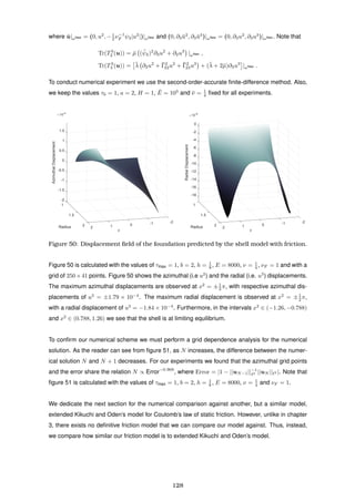
![4.6 4.8 5 5.2 5.4 5.6
log(N)
-5.3
-5.2
-5.1
-5
-4.9
-4.8
-4.7
-4.6
-4.5
-4.4
-4.3
log(Error)
Figure 51: Grid dependence of the shell model with friction.
4.6 Comparison against the works of Kikuchi and Oden
To extend Kikuchi and Oden [102] model, to model two-body contact problem with friction, one must
modify equation (43) (see section 5.5 (v) of Kikuchi and Oden [102]). Now, assume an elastic body
on a rough rigid surface where the fiction is governed by Coulomb’s law of static friction. Given
that one is using curvilinear coordinates, fix the purely normal stress at the contact boundary as
a constant, i.e. νF T3
3 (v)|ω = K , where K is the spring modulus. Then, equation (43) and the
analysis that is conducted in section 2.6 imply that jε(v)δv = − ω
(g33)
1
2 T3
α(v)δvα
dω, where v
is the displacement field of the elastic body. Note that v|ω describes the relative displacement
between the elastic body and the boundary ω, and thus, if the elastic body is in contact with another
rough elastic body, then the displacement field one must consider is the relative displacement, due
to the fact that friction apposes relative potential motion. Now, consider a two-body contact problem
where the contact area is rough and the friction is governed by Coulomb’s law of static friction.
Now, let the displacement fields of the overlying body be v and the foundation be u. As normal
stress is continuous at the boundary, just as before, fix the purely normal stress as νF T3
3 (u)|ω =
νF T3
3 (v)|ω = K and make the transformation vβ
→ vβ
− uβ
in the functional jε(·) to signify the
relative displacement field. Now, collecting all the tangential terms from the contact boundary (i.e.
uβ
|ω and vβ
|ω terms) one finds jε(v − u)(δv − δu) = − ω
(g33)
1
2 (T3
α(v)δvα
|ω− − T3
α(u)δuα
|ω+ ) dω,
where
jε(v − u) =
ω
(K Φ(v − u) −
1
2
ε) dω , if Φ(v − u)|ω ≥ ε ,
ω
1
2
K ε−1
Φ(v − u)2
dω , if Φ(v − u)|ω < ε ,
and where Φ(v − u) = |(vα − uα)(vα
− uα
)|
1
2 , ω+
= limx3→0+ {ω × [0, h)}, ω−
= limx3→0− Ω and
ε > 0 is the regularisation parameter.
In accordance with our previous work we keep v as the displacement field of the overlying body
and u as the displacement field of the foundation. As the two bodies are in contact, the normal
displacement, of the both bodies, is identical. Thus, one obtain the extended Kikuchi and Oden’s
129](https://image.slidesharecdn.com/a24f3df3-5be8-40a0-a0ff-910a71f94372-170108131508/85/PhDKJayawardana-135-320.jpg)
![model for Coulomb’s law of static friction for a two-body problem in curvilinear coordinates, which is
described by the equations
v3
|ω+ − u3
|ω− = 0 ,
T3
3 (v)|ω+ − T3
3 (u)|ω− = 0 ,
Tβ
3 (v)|ω+ =
−
νF (g33)
1
2 (vβ
− uβ
)
Φ(v − u)
T3
3 (v)|ω+ , if Φ(v − u)|ω+ ≥ ε ,
−
νF (g33)
1
2 (vβ
− uβ
)
ε
T3
3 (v)|ω+ , if Φ(v − u)|ω+ < ε ,
Tβ
3 (u)|ω− =
−
νF (g33)
1
2 (vβ
− uβ
)
Φ(v − u)
T3
3 (u)|ω− , if Φ(v − u)|ω− ≥ ε ,
−
νF (g33)
1
2 (vβ
− uβ
)
ε
T3
3 (u)|ω− , if Φ(v − u)|ω− < ε ,
where
Tβ
3 (v) = µ ¯ β
v3 + ¯3vβ
,
T3
3 (v) = λ ¯αvα
+ (λ + 2µ) ¯3v3
,
Tβ
3 (u) = ¯µ ¯ β
u3 + ¯3uβ
,
T3
3 (u) = ¯λ ¯αuα
+ ¯λ + 2¯µ ¯3u3
,
and where λ and µ are respectively first and second Lame’ parameters of the overlying body, ¯λ and
¯µ are respectively first and second Lame’ parameters of the foundation, and νF is the coefficient of
friction. Note that in this framework one has g33 = 1. Also, given that T3
3 (u)|ω− is fixed as a positive
constant and one is considering Euclidean coordinates, one can see that the above problem simply
reduces to Kikuchi and Oden’s [102] model for Coulomb’s law of static friction in the limit u → 0.
Despite the fact that we are working in linear elasticity, the above equations make our problem in-
herently nonlinear. Thus, to find numerical solutions we employ the Newton’s method for nonlinear
systems (see chapter 10 of Burden et al. [30]).
To conduct numerical experiments consider the following. In accordance with the framework that is
introduced in section 3.5, the overlying body is restricted to the region x3
∈ (0, h). Thus, with some
calculations, one finds that the perturbed governing equations of the overlying body are
(λ + µ)∂2 ¯iδvi
+ µ ¯∆δv2
= 0 ,
(λ + µ)∂3 ¯iδvi
+ µ ¯∆δv3
= 0 ,
where
¯2δv2
= ∂2δv2
+ ¯Γ2
22δv2
+ ¯Γ2
23δv3
,
¯2δv3
= ∂2δv3
− ( ¯ψ2)2 ¯Γ2
23δv2
,
¯3δv2
= ∂3δv2
+ ¯Γ2
23δv2
,
¯3δv3
= ∂3δv3
,
130](https://image.slidesharecdn.com/a24f3df3-5be8-40a0-a0ff-910a71f94372-170108131508/85/PhDKJayawardana-136-320.jpg)
![and δv = (0, δv2
(x2
, x3
), δv3
(x2
, x3
)) is a small perturbation of the displacement field of the overlying
body. With relative ease, one finds that the perturbed governing equations of the foundation are
(¯λ + ¯µ)∂2 ¯iδui
+ ¯µ ¯∆δu2
= 0 ,
(¯λ + ¯µ)∂3 ¯iδui
+ ¯µ ¯∆δu3
= 0 ,
where δu = (0, δu2
(x2
, x3
), δu3
(x2
, x3
)) is the perturbation of the displacement field of the founda-
tion. With some more calculations, one finds the following boundary conditions to the displacement
fields,
v3
− u3
|ωNew = 0 (continuous radial displacement) ,
T3
3 (v) − T3
3 (u) |ωNew = 0 (continuous radial stress) ,
and the boundary conditions for the perturbations
δu2
|∂ΩNew
0 ∪∂Ω
New
f
= 0 ,
δu3
|∂Ω
New = 0 ,
δv2
|{∂ωNew×(0,h)}∪{[− 1
2 π, 1
2 π]×{h}} = 0 ,
δv3
|¯ωNew∪{∂ωNew×(0,h)}∪{[− 1
2 π, 1
2 π]×{h}} = 0 .
Thus, the equations characterising the frictionally coupling of the overlying body to the foundation
can be expressed as:
If ¯ψ2|v2
− u2
||ωNew ≥ , then
µ ¯ψ2∂3v2
+ ( ¯ψ2)−1
∂2v3
+ νF sign(v2
− u2
)T3
3 (v) |ωNew = 0 ,
¯µ ¯ψ2∂3u2
+ ( ¯ψ2)−1
∂2u3
+ νF sign(v2
− u2
)T3
3 (u) |ωNew = 0 ;
If ¯ψ2|v2
− u2
||ωNew < , then
µ ¯ψ2∂3δv2
+ νF
−1 ¯ψ2(v2
− u2
)T3
3 (δv) + νF
−1 ¯ψ2(δv2
− δu2
)T3
3 (v)
+ µ ¯ψ2∂3v2
+ ( ¯ψ2)−1
∂2v3
+ νF
−1 ¯ψ2(v2
− u2
)T3
3 (v) |ωNew = 0 ,
¯µ ¯ψ2∂3δu2
+ νF
−1 ¯ψ2(v2
− u2
)T3
3 (δu) + νF
−1 ¯ψ2(δv2
− δu2
)T3
3 (u)
+ ¯µ ¯ψ2∂3u2
+ ( ¯ψ2)−1
∂2u3
+ νF
−1 ¯ψ2(v2
− u2
)T3
3 (u) |ωNew = 0 ,
where
T3
3 (v) = λ ∂2v2
+ ¯Γ2
22v2
+ ¯Γ2
23v3
+ (λ + 2µ)∂3v3
,
T3
3 (u) = ¯λ ∂2u2
+ ¯Γ2
22u2
+ ¯Γ2
23u3
+ (¯λ + 2¯µ)∂3u3
.
To conduct numerical experiments we use the second-order-accurate finite-difference method in
conjunction with Newton’s method for nonlinear systems, as in section 2.6. Also, we keep the
values τ0 = 1, a = 2, H = 1, ¯E = 103
and ¯ν = 1
4 fixed for all experiments. Furthermore, we
choose to terminate our iterating process once the condition |1 − (||um|| 2 + ||vm|| 2 + ||δum|| 2 +
||δvm|| 2 )−1
(||um+1|| 2 +||vm+1|| 2 +||δum+1|| 2 +||δvm+1|| 2 )| < 10−10
is satisfied, where um, vm,
131](https://image.slidesharecdn.com/a24f3df3-5be8-40a0-a0ff-910a71f94372-170108131508/85/PhDKJayawardana-137-320.jpg)
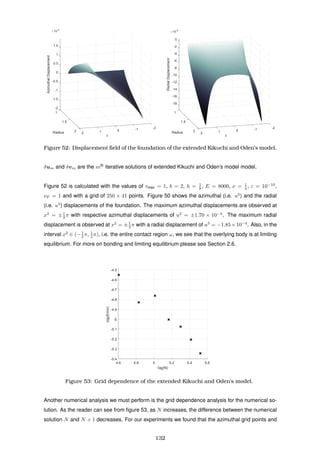
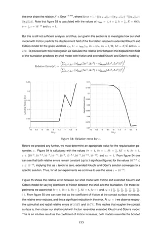

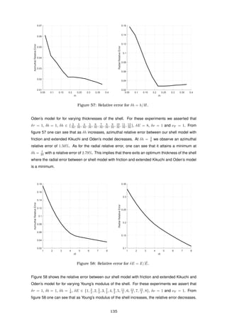
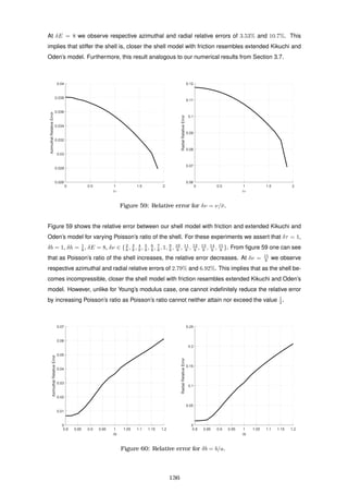
![Figure 60 shows the relative error between our shell model with friction and extended Kikuchi and
Oden’s model for varying vertical radii of the contact region. For these experiments we asserted
that δτ = 1, δb ∈ {32
40 , 33
40 , 34
40 , 35
40 , 36
40 , 37
40 , 38
40 , 39
40 , 1, 41
40 , 42
40 , 43
40 , 44
40 , 45
40 , 46
40 , 47
40 , 48
40 }, δh = 1
8 , δE = 8, δν = 1
and νF = 1. From figure 60 one can see that as the critical parametric-latitude increases, both
azimuthal and radial relative error also increases. At δb = 4
5 , we observe respective azimuthal and
radial relative errors of 0.654% and 1.07%. This implies that lower the critical parametric-latitude of
the contact region is, closer the shell model with friction resembles extended Kikuchi and Oden’s
model.
The above analyses show how the displacement field of an elastic foundation modelled with our
overlying shell, on an elastic foundation subjected to the hypothetical displacement-based friction
condition, model relative to Kikuchi and Oden’s [102] model, extended to model fully two-body
contact problem in curvilinear coordinates. However, unlike in chapter 3, there exists no definitive
two-body friction theorem (or at least a model) that we can compare our results against. Hence, the
reason we investigated the relative errors between the two solutions to see how they fair against a
set of variables.
The disadvantage of extended Kikuchi and Oden’s model is that it is unsuitable for modelling thin
overlying bodies, as the thickness of overlying body becomes infinitesimally small relative to the
thickness of the foundation, it is numerically impractical to model the overlying body as a three-
dimensional object. Thus, in this scenario extended Kikuchi and Oden’s model breaks down. This
justifies the existence of our overlying shell model with friction as this model is numerically valid for
such cases.
We again remind the reader that the physical validity of each model is still an open question as
there exits no definitive friction model that we can compare our results against. We further remind
the reader that the model we presented in this section is not a model that is derived by Kikuchi and
Oden [102]. We taken the model for Coulomb’s law of static friction from Kikuchi and Oden [102]
(see Section 1.11) and extended to curvilinear coordinates (see Section 2.6) which is then extended
to model a full two-body problem in this section. We merely called it extended Kikuchi and Oden’s
model for convenience.
4.7 Conclusions
In this chapter we studied frictionally coupled overlying shells supported by elastic foundations. In
Section 4.2 we used Kikuchi and Oden’s [102] model for Coulomb’s law of static friction to derive
a displacement-based static friction condition. By construction this displacement-based hypotheti-
cal friction condition is more mathematically sound than Coulomb’s law, but its physical validity still
remains an open question. Then, in Section 4.3, we explicitly derived the governing equations and
the boundary conditions for the general case for overlying shells on elastic foundations when sub-
jected to a displacement-based friction condition. In Section 4.4 we used the work of Evans [63]
137](https://image.slidesharecdn.com/a24f3df3-5be8-40a0-a0ff-910a71f94372-170108131508/85/PhDKJayawardana-143-320.jpg)
![and, Kinderlehrer and Stampacchia [107] to prove the existence and the uniqueness of the solu-
tions, and thus, proving that what we derived is a mathematical theory and not a hypothetical model.
In chapter 4.5 we presented framework to conduct a set of numerical solutions. For numerical anal-
ysis, in Section 4.6, we extended Kikuchi and Oden’s [102] model for Coulomb’s law of static friction
to model a full two-body contact problem in curvilinear coordinates and shown how numerical solu-
tions fair against our shell model with friction. The method of numerical analysis is to ascertain how
the displacement field of the foundation behave when the overlying body is modelled by our shell
model with friction relative to extended Kikuchi and Oden’s model. The numerical analysis shows
that, if the shell is thick, the shell is stiff, the shell is close to incompressible, contact region has
a very high coefficient of friction or contact region has a low critical parametric-latitude, then the
displacement field of the foundation predicted by both models be in better agreement.
From our numerical analysis the greatest reduction in the error is observed for higher coefficients
of friction, i.e. as the coefficient of friction increases, the bodies behaves as if they are bonded,
and thus, the greater agreement between the solutions of extended Kikuchi and Oden’s model
and our shell model with friction. This is an expected result as we initially derived our overlying
shell model to approximate bonded thin bodies on elastic foundations, and the efficacy of our initial
model is numerically modelled in Sections 3.6 and 3.7. The second greatest reduction in the error
is observed for higher Young’s moduli of the shell. This is also an expected result as we observed in
Section 3.7 that the overlying shell models are mostly accurate for shells with relatively high Young’s
moduli.
138](https://image.slidesharecdn.com/a24f3df3-5be8-40a0-a0ff-910a71f94372-170108131508/85/PhDKJayawardana-144-320.jpg)
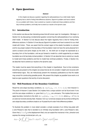
![+
1
2
E
x0
−x0
h(∂xu1
)2
+
1
3
h3
(∂xxu3
)2
dx
+ h(τ1
0 u1
+ τ3
0 u3
)|(x,z)=(−x0,0) − h(τ1
0 u1
+ τ3
0 u3
)|(x,z)=(x0,0) , ∀ (v1
, v3
) ∈ VP(ω, Ω) ,
where
VP(ω, Ω)={(v1
, v3
) ∈ H1
(Ω) | (v1
, v3
) ∈ H1
(ω)×H2
(ω)|ω, (v1
, v3
)|z=−H =0, ∂xu3
|(x,z)=(±x0,0) =0} ,
and where ¯E is Young’s modulus and H is the thickness of the foundation, E is Young’s modulus
and h is the thickness of the plate, τ1
0 , τ3
0 ∈ R are constant tractions, Ω = (−x0, x0) × (−H, 0) and
ω = (−x0, x0). It can be shown that the above problem has a unique minimiser, which is also a
critical point. Thus, assuming that u1
∈ C2
(Ω), u3
∈ C2
(Ω), u1
|ω ∈ C2
(ω), and u3
|ω ∈ C4
(ω) one
can express the governing equations of the problems as
∂xxu1
+
1
2
∂zzu1
+
1
2
∂xzu3
|Ω = 0 ,
1
2
∂xzu1
+
1
2
∂xxu3
+ ∂zzu3
|Ω = 0 ,
∂xxu1
−
¯E
hE
(∂zu1
+ ∂xu3
) |ω = 0 ,
∂xxxxu3
+ 3
¯E
h3E
∂zu3
|ω = 0 ,
and the boundary conditions of the problems as
(u1
, u3
)E|(x,z)∈{[−x0,x0]×{−H}} = 0 , ∂xu3
|(x,z)=(±x0,0) = 0 ,
∂xu1
|(x,z)∈{{±x0}×(−H,0)} = 0 , ∂xu1
|(x,z)=(±x0,0) = 2
τ1
0
E
,
∂zu1
+ ∂xu3
|(x,z)∈{{±x0}×(−H,0)} = 0 , ∂xxxu3
|(x,z)=(±x0,0) = −6
τ3
0
h2E
.
The above problem has a unique numerical solution. However, if one omit the zero-slope bound-
ary conditions, i.e. ∂xu3
|(x,z)=(±x0,0) = 0, then one can impose an arbitrary boundary moment as
∂xxu3
|(x,z)=(±x0,0) = 2E−1
η0, where η0 ∈ R is a constant external moments density. However, if one
numerically models this problem with the boundary moments, i.e. without the zero-slope boundary
conditions, then the numerical scheme fails to converge. Hint: consider the change of variables
(w1
(x), w3
(x))E = (∂xxu1
(x, z), ∂xxu3
(x, z))E|ω for the numerical scheme.
It is unclear that if are making a mistake in the proof of theorem 3 or we are not correctly numerically
modelling the problem. If it is the proof, then the problem must lie in the rigid displacement result
from Section 3.4, or, if it is the numerical modelling, then the problem must lie in the boundary up-
dating approach in the finite-difference scheme. Unfortunately, our knowledge in weighted Sobolev
spaces is not sufficient to investigate this problem further. For possible solutions a comprehensive
analytical treatment of boundary conditions for higher-order elliptic equations can be found in chap-
ters 3 and 6 of Necas et al. [144] and an analysis of finite-difference schemes for fourth-order elliptic
differential operators can be found in section 2.7 of Jovanovic and Suli [93].
5.3 Regularity
Regularity is very important when finding numerical solutions. For example, one requires the min-
imiser of the energy functional to have higher regularity in order to construct finite-difference solu-
140](https://image.slidesharecdn.com/a24f3df3-5be8-40a0-a0ff-910a71f94372-170108131508/85/PhDKJayawardana-146-320.jpg)
![tions. But in our framework that we presented in chapters 3 and 4 only finite-element solutions can
be mathematically justified. Yet, we know the existence of finite-difference solutions due to numeri-
cal analysis. Can one prove the existence of higher regularity solutions with sufficient mathematical
rigour?
To investigate this matter further recall theorem 3. The set VS (ω, Ω) is a linear set as any finite
linear combination of the elements in the set belongs to the set. Now, let ¯X ∈ C3
(¯Ω; E3
) and let
∂Ω be a uniform-C3
(R2
; R) boundary (see section 4.10 of Adams [3]). Then, a possible minimiser
u of J(·), maybe written as u = u0 + ˜u where u0 ∈ H1
0(Ω) and ˜u ∈ H2
(Ω)×H2
(Ω)×H3
(Ω). Note
that the latter condition follows from the boundary trace embedding theorem (see theorem 5.36
of Adams [3]) and Rellich-Kondrachov theorem (see theorem 6.3 of Adams [3]), i.e. we have the
compact embeddings H2
(Ω) → H1
(ω) and H3
(Ω) → H2
(ω). Clearly, we still have u ∈ VS (ω, Ω).
Now, if we let f ∈ H1
(Ω)×H1
(Ω)×H2
(Ω), then from theorem 3.9-4 of Ciarlet [39] (for proof see
Agmon et al. [5] and Geymonat [75]) we obtain u0 ∈ H2
(Ω)×H2
(Ω)×H3
(Ω). This implies that
u ∈ H2
(Ω)×H2
(Ω)×H3
(Ω).
Note that our problem is a displacement-traction problem: it is displacement due to u|∂Ω0 = 0 and
traction due to τ0. Thus, we require much finer analysis on trace spaces and fractional order spaces.
Luckily, comprehensive analysis of fractional order spaces can be found in chapter 7 of Adams [3]
and analysis on the regularity of solutions can be found in chapter 4 of Necas et al. [144]. Thus, it
may be possible for one to construct a proof such that u ∈ C3
(Ω)×C3
(Ω)×C4
(Ω), which is sufficient
for proving the existence of finite-difference solutions.
But does this mean that the every minimiser of J(·) has the form u = u0 + ˜u, where u0 ∈ H1
0(Ω)
and ˜u ∈ H2
(Ω)×H2
(Ω)×H3
(Ω), or that the form u = u0 + ˜u satisfies any minimising solution:
certainly not! Without a firm proof everything we discussed regarding the higher order regularity is
merely speculative. One requires more sophisticated analysis to solve this regularity problem.
5.4 Signorini’s Problem
Signorini’s problem describes the contact of a linearly elastic body with a rigid frictionless foundation
where the solution describes the displacement field of the elastic body at the contact region as well
as the range of the contact region, as the contact region is also considered as a part of the solution.
On a historical note the general problem of the equilibrium of a linearly elastic body in contact with
a rigid frictionless foundation is initially introduced by Signorini [178, 179].
Characterisation of Signorini’s problem is as follows: consider a three-dimensional linearly elastic
body, which is described by the displacement field v, in contact with a rigid foundation. Let ΓC ⊂ ∂Ω
be the candidate contact surface. Note that the actual surface on which the body comes in contact
with the foundation is not known in advance, but it is assumed that it is contained in the candidate
contact surface as a proper subset. Now, let ψ be the initial relative displacement field between the
141](https://image.slidesharecdn.com/a24f3df3-5be8-40a0-a0ff-910a71f94372-170108131508/85/PhDKJayawardana-147-320.jpg)
![elastic body and the rigid foundation. This leads the following equations at the candidate contact
surface,
¯niTi
j (v) − ¯ni¯nk
Ti
k(v) |ΓC
= 0 , ∀ j ∈ {1, 2, 3} ,
¯ni¯nk
¯nlTi
k(v)(vl
− ψl
)|ΓC
= 0 ,
¯ni(vi
− ψi
)|ΓC
≤ 0 ,
¯ni¯nk
Ti
k(v)|ΓC
≤ 0 ,
where ¯n is the unit outward normal to ΓC.
To extend Signorini’s problem to a shell supported by an elastic foundation consider the method
for a pseudo-two-body contact problem described in section 6.8 of Kikuchi and Oden [102]. Armed
with this knowledge, let u describe the displacement field of the shell. Now, assume that this
shell is in contact with an elastic foundation with a frictionless boundary. We use the curvilinear
coordinate system of the shell as the coordinate system of the elastic foundation, and given that the
lower-surface of the shell satisfies assertion 1, we asserts that the foundation is located beneath
the lower-surface of the shell. Now, let v be the displacement field of the foundation and let ψ
be the initial relative displacement field between shell and the foundation, which is a known field in
advance. Thus, the energy functional of a shell with a thickness h on a frictionless elastic foundation
may have the form
J(u, v) =
Ω
1
2
Aijkl
Eij(v)Ekl(v) − fi
vi dΩ
+
ω
1
2
Bαβγδ
h αβ(u) γδ(u) +
1
3
h3
ραβ(u)ργδ(u) − hfi
0ui dω
−
∂ω∂ω0
hτi
0 ui +
1
3
h3
ηα
0 αu3
d(∂ω) , ∀ (u, v) ∈ V Signorini(ω, Ω) ,
where
V Signorini(ω, Ω) = {u ∈ V Shell(ω), v ∈ V Foundation(Ω) | ¯ni(vi
− ui
− ψi
)|ΓC
≤ 0} ,
V Shell(ω) = {u ∈ H1
(ω)×H1
(ω)×H2
(ω) | u|∂ω0
= 0, nα
∂αu3
|∂ω0
= 0} ,
V Foundation(Ω) = {v ∈ H1
(Ω) | v|∂Ω0
= 0} ,
¯n is the unit outward normal to the boundary ∂Ω and n is the unit outward normal to the boundary
∂ω in curvilinear coordinates. Note that Ω ⊂ R3
is a connected open bounded domain with a suffi-
ciently smooth boundary ∂Ω such that ΓC, ∂Ω0 ⊂ ∂Ω, where ¯ΓC ∩ ¯∂Ω0 = Ø with meas(∂Ω0; R2
) > 0.
Also, ω ⊂ R2
is a connected open bounded plane with a sufficiently smooth boundary ∂ω such
that ∂ω0 ⊂ ∂ω with meas(∂ω0; R) > 0. Furthermore, f ∈ L2
(Ω), f0 ∈ L2
(ω), τ0 ∈ L2
(∂ω) and
η0 ∈ L2
(∂ω) where η0 is a external moments density field.
For Signorini’s case we fix the displacement field of the shell in a proper subset of its boundary,
i.e. u|∂ω0 = 0 and nα
∂αu3
|∂ω0 = 0. With our previous analysis, we do not consider this condi-
tion as we treated the shell as a boundary form. But, now the shell is a separate body, and thus,
we must assert the current condition to keep the problem static and to avoid a pure-traction problem.
142](https://image.slidesharecdn.com/a24f3df3-5be8-40a0-a0ff-910a71f94372-170108131508/85/PhDKJayawardana-148-320.jpg)
![Thus far we only considered smooth contact surfaces. But, what if the contact surface is no longer
smooth? To extend to above problem to include friction consider Signorini’s problem with Coulomb’s
law of static friction that is described in section 10.2 of Kikuchi and Oden [102]. Using Kikuchi and
Oden’s model as inspiration, we extend hypothesis 3 by considering the relative displacements
between the shell and the elastic foundation. Thus, the energy functional of a shell with a thickness
h on a elastic foundation with a displacement-based friction condition may have the form
J(u, v) =
Ω
1
2
Aijkl
Eij(v)Ekl(v) − fi
vi dΩ
+
ω
1
2
Bαβγδ
h αβ(u) γδ(u) +
1
3
h3
ραβ(u)ργδ(u) − hfi
0ui dω
−
∂ω∂ω0
hτi
0 ui +
1
3
h3
ηα
0 αu3
d(∂ω) , ∀ (u, v) ∈ V Friction(ω, Ω) ,
where
V Friction(ω, Ω)={(u, v) ∈ V Signorini(ω, Ω) | 2νF ¯n·(v−u−ψ) + |(v−u−ψ) − ¯n·(v−u−ψ)| |ΓC
≤ 0} ,
and νF is the coefficient of friction between the elastic foundation and the shell. Note that u·v = uivi
and |v| = (vivi
)
1
2 for any vectors u, v in the curvilinear space.
Can we guarantee that the above problems even have solutions? Certainly not. Even Kikuchi and
Oden’s [102] (frictionless) two-body problem is not necessarily a two-body problem. It is a much
simpler problem where a single elastic body folded in on itself so one only needs to deal with a
single displacement field (see section 6.8 of [102]). However, even the single body case is given
as a hypothetical model as the existence and the uniqueness of solutions are not proven by the
authors. The problems that we present may have solutions, but without proving the existence of
solutions with rigorous mathematics this remains a merely an interesting hypothetical model.
For further information on the subject we direct the reader to chapter 6 of Kikuchi and Oden [102]
for rigorous analysis of Signorini’s problem, where the authors meticulously present the mathemat-
ical framework for a variational statement of Signorini’s problem, and prove the existence and the
uniqueness of solutions. Just let g = niψi
to be consistent with Kikuchi and Oden’s [102] termi-
nology. Among other finer analyses the authors also present a finite-element approximation that
is developed for the exterior penalty formulation of Signorini’s problem using 9-node isoparametric
quadrilateral elements, and give many solved examples with the use of the finite-element penalty
method. Furthermore, extensions to Signorini’s problem, such as the elastic pseudo-two-body con-
tact problem, can be found in section 6.8 of the publication and Signorini’s problem with Coulomb’s
law with static friction can be found in section 10.2 of the publication.
5.5 Nonlinear Elasticity
Nonlinear elastic problems are an immensely important branch in the field of mathematical elasticity.
For example, large deformation of elastic bodies cannot accurately be modelled by linear elasticity
as the latter method is only valid for infinitesimal deformations. Nonlinear elasticity models require
143](https://image.slidesharecdn.com/a24f3df3-5be8-40a0-a0ff-910a71f94372-170108131508/85/PhDKJayawardana-149-320.jpg)
![finite deformation modelling, also it is sometimes the case in mathematical elasticity that certain
results in linear elasticity cannot be mathematically justified as it can be with hyperelasticity (see
section 2 subsection 7.7 of Morassi and Paroni [139] for the examples of convexity and policonvex-
ity). Furthermore, certain forcings of the elastic body may depend on the displacement field, and
thus, making the force density a function of the displacement field (for examples of such problems,
please see chapter 2 section 4 Lions [123]). For such problems analysis in linear elasticity is insuf-
ficient, and thus, one must extend the work to nonlinear mathematical elasticity.
Now, recall theorem 3 or 4 and consider the field f for an example. Thus far we only considered
the case f = f(x1
, x2
, x3
), but not f = f(u). But, what if the latter is the problem in question?
If this the case, then we are dealing with a semi-linear problem. For example, assume that there
exists a constant C that depends on Ω and ¯X such that Ω
|f(u)| dΩ ≤ C||u||L2(Ω). Given that C
is sufficiently small, one may show the existence of solutions with slight modification of the proof for
theorem 3. However, it is unclear how this new term will affect Korn’s inequality, and thus, we do
not assert any strong claims regarding existence of minimisers with any certainty. Instead, we refer
the reader to the publication by Badiale and Serra [13] for an in-depth study of existence results for
semi-linear elliptic equations using the variational approach.
To study finite deformations, or even to study Signorini’s problem that we present in Section 5.4
accurately, one must move to the realm of fully nonlinear problems. To examine this further consider
the map
¯r(v) = ¯X + vi
∂i
¯X ,
where v = v(x1
, x2
, x3
) is the displacement field of the foundation. Thus, nonlinear Green-St Venant
strain tensor components can be expressed as
Eij(v) =
1
2
∂i¯rk(v)∂j ¯rk
(v) − ∂i
¯Xk∂j
¯Xk
.
Armed with this knowledge, one can express the stored energy density as
W(v) =
1
2
Aijkl
Eij(v)Ekl(v) .
As the stored energy density W(·) is a scalar, any change of coordinates to the Euclidean coordinate
system will not affect the energy density. Thus, if one make this transformation, then one can easily
show that the stored energy density is policonvex, i.e. there exists a convex functional
Z : M3×3
× M3×3
× R → R ,
such that
W(v) = Z( ¯EvE, cof( ¯EvE), det( ¯EvE)) ,
where ¯E is the differential operator in the Euclidean space, vE = vi
∂i
¯X is a Euclidean displace-
ment field, and cof(M) = (det M)M−T
, ∀ M ∈ M3×3
, is the cofactor of a matrix and M3×3
is the
space of 3 × 3 matrices. For more on policonvexity please consult section 2 of Morassi and Paroni
144](https://image.slidesharecdn.com/a24f3df3-5be8-40a0-a0ff-910a71f94372-170108131508/85/PhDKJayawardana-150-320.jpg)
![[139].
Existence of a minimiser can be shown using the techniques from the study of hyperelasticity. The
first ever successful proof is derived by Ball [17], where the author also proves the existence of min-
imisers for displacement-traction problems and pure-traction problems. If the reader wishes to see
the proof of the existence of minimisers for a unilateral boundary condition of place problem, prob-
lems of self-contact without friction and of non-interpenetration matter, then please consult chapter
7 of Ciarlet [36].
Now, consider the map
r(w) = R(w) + x3 ∂1R(w) × ∂2R(w)
||∂1R(w) × ∂2R(w)||
,
where R(w) = σ + wα
∂ασ + w3
N and w = w(x1
, x2
) is the displacement field with respect to the
mid-surface of the shell. Thus, the nonzero nonlinear strain tensor components can be expressed
as
eαβ(w) =
1
2
∂αri(w)∂βri
(w) − ∂α(σi +x3
Ni)∂β(σi
+x3
Ni
) .
With some further calculations, one can show that
e(w) = (w) − x3
ρ(w) ,
where
αβ(w) =
1
2
∂αRi(w)∂βRi
(w) − ∂ασi∂βσi
,
ραβ(w) = ∂αβRi(w)
(∂1R(w) × ∂2R(w))i
||∂1R(w) × ∂2R(w)||
− Ni∂αβσi
,
(see chapter 4 of Ciarlet [39]). Armed with this knowledge, one can express the stored energy
density of a nonlinear shell with a thickness 2h as
wmid
2h (w) =
1
2h
h
−h
1
2
Bαβγδ
αβ(w) − x3
ραβ(w) γδ(w) − x3
ργδ(w) dx3
.
Thus, for an overlying nonlinear shell with a thickness h (see hypothesis 2) the stored energy density
is
wlow
h (u) =
1
2
Bαβγδ
αβ(u) γδ(u) +
1
3
h2
ραβ(u)ργδ(u) ,
i.e. wlow
h (u) = wmid
2h (w), where u = u(x1
, x2
) is the displacement field with respect to the lower-
surface. It can be proven by Γ-convergence that the three-dimensional hyperelastic body tends
to the nonlinear shell problem as the thickness approaches zero. As the existence of a minimiser
can be proven for three-dimensional hyperelastic bodies, Γ-convergence automatically provides the
existence of a minimiser for nonlinear shells. For the proof please consult section 2.5 of Ciarlet and
Mardare [40]. Note that the first rigorous proof of this approach is presented by Dret ans Raoult
[114], and Friesecke et al. [66]. For more on Γ-convergence please consult section 3 of Morassi
and Paroni [139].
145](https://image.slidesharecdn.com/a24f3df3-5be8-40a0-a0ff-910a71f94372-170108131508/85/PhDKJayawardana-151-320.jpg)
![Separately we can prove the existence of weak solutions for nonlinear shells and three-dimensional
hyperelastic bodies. But the question is: can we prove the existence of a weak solution for a non-
linear shell supported by a hyperelastic foundation, either as a two-body problem as in Signorini’s
problem case (see Section 5.4) or as the nonlinear shell as a boundary form of the hyperelastic
foundation case (analogous to chapters 3 and 4)? The answer is no. This problem requires more
sophisticated analysis, and thus, we leave it as future work.
5.6 Dynamic Case
In this section we discuss the evolution equations of shells supported by elastic foundations. Con-
sider a real-life scenario where one applies an unbalanced force and or a moment to an overlying
shell on an elastic foundation. How will it behave?
For our framework we assumed that our shell and the elastic body in question are isotropic and
homogeneous, and thus, there exist two positive constants and ¯ such that they are the mass
densities of the respective bodies. Now, assume that our problem in question evolves within the
time interval [0, T], where T > 0. Now, let ΩT = Ω×(0, T), ωT = ω×(0, T) and ∂ωT = ∂ω×(0, T).
Given that we are considering Signorini’s problem (so no boundary forms), let u = u(x1
, x2
, t)
be the displacement of the shell and v = v(x1
, x2
, x3
, t) be the displacement of the elastic foun-
dation. For convenience, assume that the initial and the final first-order partial derivatives of the
displacement field with respect to time of both bodies are zero, i.e. (∂tv1
, ∂tv2
, ∂tv3
)|t∈{0,T } = 0
and (∂tu1
, ∂tu2
, ∂tu3
)|t∈{0,T } = 0. Thus, one can express the action functional of a shell with a
thickness h on an elastic foundation as
S(u, v) =
ΩT
1
2
Aijkl
Eij(v)Ekl(v) − fi
vi −
1
2
¯∂tvi∂tvi
dΩT
+
ωT
1
2
Bαβγδ
h αβ(u) γδ(u)+
1
3
h3
ραβ(u)ργδ(u) − hfi
0ui
−
1
2
h∂tui∂tui
−
1
3
h3
ρα
α(∂tu)∂tu3
dωT
−
∂ωT
hτi
0 ui −
1
3
h3
ηα
0 (∂ασ) ·
∂1R(u) × ∂2R(u)
||∂1R(u) × ∂2R(u)||
d(∂ωT ) ,
with the displacement fields satisfying the conditions
v|∂Ω0
= 0 (Zero displacement condition) ,
v|Ω×{0} = 0 (Initial condition of the foundation) ,
u|ω×{0} = 0 (Initial condition of the shell) ,
¯n·(v−u−ψ)|ΓC
≤ 0 (Signorini’s condition) ,
2νF ¯n·(v−u−ψ) + |(v−u−ψ) − ¯n·(v−u−ψ)| |ΓC
≤ 0 (Displacement-based friction condition) ,
where ∂t is the partial derivative with respect to time. Note that ∂t¯r(v) · ∂t¯r(v) = ∂tvi∂tvi
and
1
2h
h
−h
∂tr(u) · ∂tr(u) dx3
= ||∂t uα
∂ασ + u3
N ||2
+
1
3
h2
∂t
∂1R(u) × ∂2R(u)
||∂1R(u) × ∂2R(u)||
2
,
= ∂tuα∂tuα
+ ∂tu3∂tu3
−
1
3
h2
ρα
α(∂tu)∂tu3
.
146](https://image.slidesharecdn.com/a24f3df3-5be8-40a0-a0ff-910a71f94372-170108131508/85/PhDKJayawardana-152-320.jpg)
![As we are dealing with curvilinear coordinates, integrating by parts with respect to the time variable
leads the appearance of Christoffel symbols, despite that both the diffeomorphism and the injective
immersion are independent of time, i.e. ¯X(x1
, x2
, x3
) = ¯X(x1
, x2
, x3
, t) and σ(x1
, x2
) = σ(x1
, x2
, t)
(see section 7.6 of Kay [101]). Armed with this knowledge, and the fact that we are assuming that
the initial and the final first-order partial derivatives of the displacement fields with respect to time
of both bodies are zero, we get the following relation in the foundation,
ΩT
∂tvi∂tvi
dΩT = −
ΩT
∂ttvi
+ ¯Γi
kl∂tvk
∂tvl
vi dΩT ,
and the following relation in the shell,
ωT
∂tuα∂tuα
+ ∂tu3∂tu3
dωT = −
ωT
∂ttuα
+ Γα
γδ∂tuγ
∂tuδ
− 2F α
[II]γ ∂tuγ
∂tu3
uα
+ ∂ttu3
+ F[II]αγ∂tuα
∂tuγ
u3 dωT .
As one can see that to accurately model this problem, one needs to consider the nonlinear case.
Also, notice that for the dynamic case one do not assert zero-Dirichlet and the zero-slope of the
displacement field of the shell in a proper subset of its boundary, as now one may allow the shell to
move freely without any mathematical restrictions due its dynamic nature.
The crucial question is that can we prove the existence of solutions to the dynamic problem? The an-
swer is no. Fortunately, a comprehensive analysis on vibration of shells can be found in Leissa [115]
and Soedel [181]. For shell-membranes, an asymptotic justification for the equations of dynamic
shell-membranes can be found in Xiao [212]. Furthermore, there is a vast number of publications
in the study of dynamic elastic problems in Euclidean coordinates, particularly in plate theory. For
example, a thorough numerical analysis of the dynamical rectangular plates can be found in section
9 of Reddy [163]. Note that, if we consider the linear case, then the dynamic problem we present
in this section is a hyperbolic problem. For elementary analysis on hyperbolic equations can be
found in section 7.2 and section 11.1.2 of Evans [63]. But, for a more in-depth analysis of evolution
problems please consult Lions [123].
5.7 Conclusions
In this chapter we presented possible future research topics as open questions. These open ques-
tions are areas that we did not study with mathematical rigour due to time constraints and lack
of pre-existing research material. Above, we described a fundamental issue concerning the well-
posedness of our overlying shell model. We also explored: (i) means to extend the regularity of
the weak solutions of the theorem 3 to higher regularity, (ii) means to extend Signorini’s problem
to overlying shells on elastic foundations with friction, (iii) means to extend the problem to either
semi-linear case or nonlinear case or both, and (iv) means to extend the problem to the dynamic
case. Although, we did not prove the existence of solutions for any of the cases that we presented
or, at least, give any numerical solutions, we did meticulously document the necessary literature to
consult so that the reader may prove or disprove the given formulations.
147](https://image.slidesharecdn.com/a24f3df3-5be8-40a0-a0ff-910a71f94372-170108131508/85/PhDKJayawardana-153-320.jpg)
![6 Modelling Skin Abrasion
Abstract
In this chapter we derive a belt-friction model for a membrane over a rigid obstacle of positive
mean-curvature. Also, we derive a static friction model for a shell-membrane supported by an
elastic foundation. Then, we use the models to process experimental data that we gathered from
human subjects to see which mechanical, elastic and geometrical factors can affect the coefficient
of friction between skin and fabrics, and the deformation field and the stress profile at the contact
area.
6.1 Introduction
In this chapter we attempt to mathematically model and experimentally investigate skin abrasion.
We begin, in Sections 6.1.1, 6.1.2 and 6.1.3, by describing various types of skin abrasion docu-
mented in the current literature. Then, we begin our mathematical modelling in Section 6.2 where
we take Kikuchi and Oden’s [102] model for Coulomb’s law of static friction for the slip case and ap-
ply it to a membrane supported by a rigid foundation to derive a belt-friction model. Then, in Section
6.3, we use this mathematical model to examine which mechanical, elastic and geometrical factors
lead to a smaller coefficient of friction in a belt-friction setting. In Section 6.4 we examine the data
that we gathered from experiments conducted on human subjects and use regression analysis to
determine the implication of using belt-friction models to calculate the coefficient of friction between
in-vivo skin and fabrics. We conclude our analysis of the experimental results by highlighting which
physical factors can significantly affect the experimental results.
In Section 6.5 we use theorem 4 and Ciarlet’s [38] theory of linear shell-membranes (see chapter
4 and 5 of Ciarlet [38]) to derive a theory for frictionally coupled static shell-membranes on elastic
foundations. Then, in Section 6.6, we use this theory to conduct numerical simulations to identify
which elastic and geometrical factors can lead to a lower shear generation at the contact area of
the overlying shell-membrane model. In Section 6.7 we examine the data that we gathered from
further experiments conducted on human subjects and compare the data against the numerical
solutions of the overlying shell-membrane model to investigate the stress profile between the fabric
and each subject’s skin. We conclude our analysis of the shell-membrane model by documenting
which elastic and geometric factors can lead to a lower shear between human skin and fabrics. The
ultimate goal is to identify which elastic and geometric factors can minimise mechanical abrasion
due to repetitive movement of fabrics over human skin, so that we may present our findings to
healthcare providers to encourage and facilitate the development of products and practices that are
less damaging to human skin.
6.1.1 Pressure Ulcers
Pressure ulcers are an area of localised cutaneous damage that is typically associated with pres-
sure from bony protuberances on aged skin. Pressure ulcers can develop when a large amount of
pressure is applied to an area of skin over a short period of time or when less pressure is applied
148](https://image.slidesharecdn.com/a24f3df3-5be8-40a0-a0ff-910a71f94372-170108131508/85/PhDKJayawardana-154-320.jpg)
![over a prolong period of time. When pressure is applied to soft tissue, it results in completely or
partially obstructed blood flow to the soft tissue, starving the tissue of oxygen and nutrients, which
eventually leads to necrosis in the affected area, and thus, an ulcer. Shear (i.e. constant and pro-
longed static friction) is also a cause, as it can pull on blood vessels that feed the skin, and thus,
restricting the blood flow. Pressure ulcers often occur in very sedentary individuals such as those
with impaired mobility, bedridden and wheelchair bound [132]. If the reader is interested in this
subject, then please consult publication by Maklebust and Sieggreen [132].
It is given that friction contributes to skin damage by stripping of the epidermal layer of the skin:
creating an environment conducive to further skin damage due to friction. An alteration in the co-
efficient of friction increases skin’s adherence to the outside surface, which can eventually leads
to wounds and infections. Note that this does not result in pressure ulcers, but it is observed in
the same settings. Also, note that the language used by authors who specialised in the study of
pressure ulcers is different to mathematicians’ language. What they referrer to as shear appears to
be a force related to static friction, and friction appears to be a force related to dynamic friction. By
the definitions of shear and friction given by Bergstrom [25], this is the only logical conclusion.
Murray et al. [142] give many preventive measures for pressure ulcers. For example, to elimi-
nate shear and friction, the authors states that to protect the exposed skin by protective dressings,
padding or sheepskin, and for those who are bedridden elevating the foot of bed to 20 degrees
when sitting to prevent sliding and maintaining the head of the bed at the lowest possible elevation,
consistent with individual’s medical condition and comfort.
It is estimated that over 400, 000 individuals will develop a new pressure ulcer annually in the UK
(mainly the elderly) and approximately 51, 000 of them will be admitted to a hospital [64]. A study
conducted in 1993 [197] shows that the cost to the NHS of treating pressure ulcers is around £180
- £321 million, which is approximately 0.4% - 0.8% of the total health spending. This figure is con-
sidered to be substantial underestimate, even allowing for inflation [22].
In 2003 Bennett et al. [22] find the cost of treating pressure ulcers in UK (excluding MRSA, surgical
interventions and litigation costs) ranges between £1.4 to £2.1 billion annually, which is over 4% of
gross NHS expenditure. The cost is deduced by estimating the daily cost of the resources required
to deliver protocols of care reflecting good clinical practice. It is estimated that each episode cost
from £1, 064 for a grade-1 ulcer (i.e. non-blanchable erythema of intact skin, include discolouration
of the skin, warmth, oedema, indurations or hardness may also be used as indicators, particularly
on individuals with darker skin) to £10, 551 for a grade-4 ulcer (i.e. extensive destruction, tissue
necrosis, damage to muscle, bone, supporting structures with or without full thickness skin loss, with
expected cost of treating critical colonisation, cellulitis and osteomyelitis). In a severe case, such as
in the case of osteomyelitis, treatment can cost on average of £16, 500 per episode per individual
patient. In cases of MRSA the costs maybe significantly higher. Due to the lack of literature it is
difficult to estimate litigation costs to the NHS related to pressure ulcer care, but one must assume
149](https://image.slidesharecdn.com/a24f3df3-5be8-40a0-a0ff-910a71f94372-170108131508/85/PhDKJayawardana-155-320.jpg)
![it be a substantial amount. For example, in the USA, The Omnibus Budget Reconciliation Act in
1987 made it easier for claimants to prove that a provider is negligent following the development of
pressure damage. Thus, between 1992 and 1996 the median settlement value following successful
litigation for negligence regarding a pressure ulcer is $279, 000 [193]. Again, this evidence strongly
indicates the fact that preventive measures are immensely important. Lowering the probability of
causing pressure ulcers leads to fewer resources are spent on treating pressure ulcers, and thus,
reducing spending in the NHS.
6.1.2 Sport Related Trauma to the Skin Due to Friction
Due to excessive movement athletes are subject to repeated mechanical trauma to the skin, which
in turn often leads to observable, documented, often painful (but never fatal) skin trauma [24]. The
following conditions are documented sports related conditions and trauma to the skin caused by
friction.
Fissure of the nipple, often referred as jogger’s nipple, is a result from repeated irritation and friction
of the nipples against a top (garment) during a prolonged period of exercise or a sporting activ-
ity. It is often experienced by runners and bicycle riders as they are exposed to the friction on the
nipple for the greatest periods of time. Once affected bleeding is common, often associated with
pain. Coating the nipples with petrolatum before running is said to be helpful. Also, it is advisable
to use talcum powder, wearing a swim suit to reduce friction or, best of all, wearing a sports-bra
[116]. Note that Powell [158] states that bicyclist’s nipple is viewed more as a thermal injury in cold
weather rather than an injury from friction.
Friction blisters are a skin condition that may occur at sites of combined pressure and friction, and
maybe enhanced by heat, moisture, or cotton socks [79]. It is often observed on weight-bearing
surfaces, and affects the feet when partaking running sports such as track, basketball and football.
It is caused by shearing frictional forces, primarily horizontal, and increased heat due to physical
exertion and humidity due to perspiration can further promotes blisters [44]. Common affected ar-
eas are joints, the tips of fingers and toes, and the heel of the foot. Preventive measures include
hardening of the skin with 10% tannic acid soaks, wearing two pairs of powdered socks, use of
protective hand and foot gear, and, above all, the use of correctly fitting sport-shoes. The use of
padding with various types of polymeric materials is discussed by Muller [141]. One of the treat-
ments presented by Scher [173] consists of draining the blister with a sterile needle and covering it
with an occlusive pressure dressing such as adhesive tape. Topical antimicrobials are advisable to
assist in preventing any secondary infection.
Traction alopecia (hair loss due to abrasion) is caused primarily by pulling force being applied to the
hair or the scalp area. Copperman [43] observes traction alopecia in a women who jogged daily
with a tight-banded wide-stripped heavy headphones. Switching to a lighter headpiece reportedly
stopped the hair loss. The author also describes alopecia in two young male break-dancers, where
constant spinning on top of the head eroded the hair shafts down to the scalp. Ely [61] observes
150](https://image.slidesharecdn.com/a24f3df3-5be8-40a0-a0ff-910a71f94372-170108131508/85/PhDKJayawardana-156-320.jpg)
![traction alopecia in a young female gymnast. The gymnast lost her hair from frontal scalp to the
occiput (the back of the head) due to constant head stands and rollovers performed on the balance
beam.
Calcaneal Petechiae, often referred as the black heal, are trauma-induced darkening lesions (acral)
of the posterior or posterolateral aspect of the heel that occurs primarily in young adult athletes
[196]. It is often observed on the feet of athletes engaged in sports such as tennis, basketball and
other sporting activities that require repetitive and rapid acceleration and deceleration [171]. It is
caused by blood being deposited in the thick stratum corneum of the edge of the heel, just above
the thick plantar skin at places where blood vessels are minimally protected by fatty tissue, due to
repeated lateral shearing forces on the epidermis (the upper most part of the skin) sliding over the
rete pegs (epithelial extensions that project into the underlying connective tissue in both skin and
mucous membranes) of the papillary dermis (uppermost layer of the dermis) [88]. These types of
lesions are also observed on the edges of the palms of weight lifters and on the balls of the thumb of
golfers. Black heel is first documented by Crissey and Peachy [51] on a group of basketball players
in 1961. Rufli [171] found black heal (referred as hyperkeratosis hemorrhagica in the publication) in
2.85% of 596 nineteen-year-old Swiss military recruits who were subjected to military drills. Duprey
[20] found an 18% prevalence in young people at a regional athletic training facility (25% males,
6% females). Black heel is often is asymptomatic (harmless); however, the diagnosis is clinically
significant as it may easily be confused with nevus (mole) or malignant melanoma, where the latter
condition can be life threatening [94].
Callus is a toughened area of skin which has become relatively thick and hard in response to re-
peated friction and or pressure. It is often occurs near bony prominences (where bones are close to
the surface) [76, 85]. Formation of calluses represents a protective response of the skin to protect
itself against further damage due to friction. However, exposure to more aggressive frictional forces
to the skin cause blisters rather than allow calluses to form. Calluses are often observed in the
hands of a gymnasts, archers, tennis players, golfers and bowlers, and on the feet of a dancers,
runners and basketball players [168].
If the reader is more interested the subject please consult Bergfeld [24]. In fact, all the conditions
described above are from Bergfeld’s [24] publication. Other conditions that Bergfeld [24] present
are tennis toe, subungual hematomas, abrasions, dermal nodules, subcutaneous nodules, striae
distensae, contact dermatitis, cutaneous infections, and dermatitis due to physical and climatic
factors.
6.1.3 Other Types Trauma to the Skin Due to Friction
It is documented that friction plays a role in the development of dermatitis in other settings. In many
cases, it is observed that friction damages the stratum corneum and the stratum basale to varying
degrees [209].
151](https://image.slidesharecdn.com/a24f3df3-5be8-40a0-a0ff-910a71f94372-170108131508/85/PhDKJayawardana-157-320.jpg)
![It is believed that friction plays a significant role in incontinence associated dermatitis as many
authors publish literature on the coefficient of friction (measuring techniques and actual measure-
ments) between human skin and fabrics in incontinence related publications [23, 48, 45, 46]. Incon-
tinence is caused by involuntary leakage of urine or loss of voluntary control of the bowels. Causes
include Polyuria (excessive urine production), muscle or nerve damage and pelvic floor dysfunction.
The NHS estimates that between 3 and 6 million adults in the UK have some degree of urinary in-
continence [200], and the prevalence is set to increase due to an aging population. It is documented
that wearing of incontinence pads over prolong periods are the very cause of the problems in incon-
tinence associated dermatitis. Despite the fact that pads absorb moisture, in many cases, the pads
acts as a barrier that prevents water from escaping. This leads to an over hydration of the stratum
corneum in the epidermis. Scheuplein and Blank [174] find an increase in skin hydration leads to in-
crease in the thickness of the stratum corneum, and thus, the weakening of the cell structure. Tests
conducted on adults and on infants show that over-hydration of the stratum corneum is responsible
for a threefold increase in the coefficient of friction. Berg [23] states that prolong wearing of pads
leads to weakening of the cell structure and an increase in the coefficient of friction that may cause
mechanical abrasion, and thus, eventually leading to dermatitis. The author shows that an increase
in skin hydration (due to pads) with the presence of urine and faecal enzymes lead to an increase
in skin permeability, skin pH (from acidity to neutral) and increase in microbial count, and this can
lead to higher aberration damage. Furthermore, Wilkinson [209] states that ill-fitting diapers cause
chafing in actively kicking infants.
Frictionally-induced fissured lesions are observed below the ears or at the side of the nose in wear-
ers of ill-fitting spectacle frames [62]. Epstein [62] documents cases of two patients diagnosed with
clinically basal-cell epithelioma-like lesions (epithelial tumour) on the ear, which was later revealed,
upon further examination, as a fissured lesion caused by rubbing ear-piece from the eyeglasses.
Contact dermatitis from clothing and attire, especially from synthetics fibber shirt collars and polo
neck jumpers, is observed, and the neck area is considered to be specifically susceptible [209]. An-
gelini [8] studies the contact allergy in a series of 165 patients with eczematous dermatitis of the feet
correlated clinically with shoe contact and found that friction is a contributor of contact dermatitis.
Dermatitis due to friction is also observed in individuals who do manual labour. White [208] states
that in those who are handling turpentine it is necessary to have friction to develop and bring out
blebs and pustules. The author also documents dermatitis intertriginous areas (areas where two
skins may touch) affecting colliers (workers on ships that are design to carry coal) and fraying of
the skin of the forearms and thighs of coal miners due to coal and stone dust. The author further
documents that cotton workers developing excoriated dermatitis (wounds), even infections of the
webs of the palms from moisture and friction. Similar lesions are observed in farmers as a result of
constant irritation from the hairs on cow udders: due to milking.
In skin already affected by medical conditions friction may worsen the problem and may lead to new
152](https://image.slidesharecdn.com/a24f3df3-5be8-40a0-a0ff-910a71f94372-170108131508/85/PhDKJayawardana-158-320.jpg)
![lesions. For example, juvenile plantar dermatitis, which is a condition with the symptoms of glazed,
shiny, and broken lamellar like scales on the skin, is often found on the frictional areas of the sides
and under surfaces of the toes and forefeet of children between 3 and 14 years of age. There is a
higher prevalence in the summer months and for those who wears synthetic socks or shoes [176].
Cowen [49] reports a case in which the lesions improved when the individual began to wear cotton
socks, which may have contributed to lowering the frictional forces experienced on the skin.
6.2 Belt-Friction model
In this section we derive a pure-traction belt-friction model to describe the behaviour of dynamic
true-membranes supported by static rigid foundations.
Let ω ⊂ R2
be a simply connected open bounded domain with the sufficiently smooth boundary
∂ω and let σ ∈ C2
(ω; E3
) be an injective immersion. Now, assume that an isotropic elastic true-
membrane is in contact with a rigid non-hyperbolic surface of positive mean-curvature such that in
the stress-free configuration of the true-membrane the contact area can be parameterised by the
immersion σ. Now, assert that the true-membrane is dynamic, but the contact area remains static
and constant as ω. Now, invoke the governing equations that is derived in chapter 2, the terminology
from Section 1.5 and the time-dependence from Section 5.6 to find
αταβ
(w) + fβ
r (w) + gβ
r = ∂ttwβ
+ Γβ
αγ∂twα
∂twγ
, (76)
F[II]αγταγ
(w) + f3
r (w) + g3
r = F[II]αγ∂twα
∂twγ
, (77)
with the boundary conditions
nαταβ
(w)|∂ω = τβ
0 , ∀ β ∈ {1, 2} , (78)
where w ∈ C2
(ω; R2
) is the displacement field and is the mass density of the true-membrane,
g ∈ C0
(ω; R3
) is an external force density field, fβ
r (w) are the shear force densities, f3
r (w) is the nor-
mal reaction density, n ∈ C0
(ω; R2
) is the unit outward normal to the boundary and τ0 ∈ C0
(ω; R2
)
is a traction field.
Note that this pure-traction problem, and thus, the boundary traction field τ0 cannot be arbitrary cho-
sen. To proceed, assume that the velocity, the acceleration and the force density fields are known
and fixed prior to the problem, and invoke the compatibility condition for pure-traction problems (see
section 1.3.4 of Necas et al. [144] or section 1.8 of Ciarlet [38]) to find
∂ω
τβ
0 uβ d(∂ω)+
ω
fβ
r (w) + gβ
r − ∂ttwβ
+ Γβ
αγ∂twα
∂twγ
uβ dω = 0 ,
∀ u ∈ {v ∈ H1
(ω) | (v) = 0} ,
where (·) is the strain tensor of the true-membrane. Note that the compatibility condition implies
that the internal forces are balanced by all the applied external forces.
153](https://image.slidesharecdn.com/a24f3df3-5be8-40a0-a0ff-910a71f94372-170108131508/85/PhDKJayawardana-159-320.jpg)
![Now, assert that the contact area is rough and the friction law governing this region is governed by
Kikuchi and Oden’s [102] model for Coulomb’s law of static friction for the slip case. Adapting this
friction law to model membranes, with the techniques introduced in Section 2.2, one finds
fβ
r (w) + νF (wαwα
)− 1
2 wβ
f3
r (w) = 0 , (79)
where νF is the coefficient of friction with respect to Coulomb’s law of friction. Now, one may
rearrange the compatibility condition and use the modified Coulomb’s law of friction (79) to find a
relationship between the coefficient of friction and the external loadings as
νF
ω
(wγwγ
)− 1
2 f3
r (w)wα
uα dω =
∂ω
τα
0 uα d(∂ω)
+
ω
gα
r − ∂ttwα
+ Γα
γδ∂twγ
∂twδ
uα dω , (80)
∀ u ∈ {v ∈ H1
(ω) | (v) = 0} .
Given that the fields (∂tw1
, ∂tw2
) and (∂ttw1
, ∂ttw2
) are known quantities prior to the problem, wβ
and fj
r (w) give one five unknowns and equations (76), (77) and (79) provide one with five equations.
Thus, the system is fully determined with respect to the boundary conditions (78). Furthermore,
condition (80) provides one with a stronger system as, if the coefficient of friction is an unknown,
then a known traction can close the system and vice versa. But does it mean that this model is valid?
The answer is no. This belt-friction model is derived from a friction law that is design to model
static bodies. We asserted that velocity and acceleration fields, (∂tw1
, ∂tw2
) and (∂ttw1
, ∂ttw2
)
respectively, are known quantities prior to the problem, but speed and the acceleration may change
during a given time interval. Finally, with our limited knowledge we cannot prove the existence of
solution for this model. The problem of proving the existence of solutions arises from the function
fβ
r (w), as it is a function of both w and w. If fβ
r (w) is a purely a function of w, then the existence
of solutions maybe proved by variational methods for semi-linear elliptic equations (see Badiale and
Serra [13]), but with the w dependence, our model is not even a variational problem. Closed
system it maybe, but this model is flawed, and thus, any result that maybe generated from this
model is merely speculative.
6.3 Numerical Analysis
To conduct numerical experiments assume a surface of revolution case, where the both contact
surface and the unstressed true-membrane parameterised by the same immersion (i.e. an aximem-
brane case). Let this immersion be σ(x1
, x2
) = (x1
, ϕ(x1
) sin(x2
), ϕ(x1
) cos(x2
))E, where x1
∈ (0, l)
and x2
∈ (−1
2 π, 0). To keep the contact area as a surface of positive mean-curvature, assert that
ϕ(x1
) = r0 − 16c(l−1
x1
− 1
2 )4
, where c < r0. Note that l, c and r0 are some positive constants that
one can specify later. With some calculations, one finds that the first fundamental form tensor is
F[I] = diag((ψ1)2
, (ψ2)2
), where ψ1 = (1+(ϕ (x1
))2
)
1
2 and ψ2 = ϕ(x1
). With a few more calculations,
one finds
Γ1
11 = (ψ1)−1
∂1ψ1 , F 1
[II]1 = (ψ1)−1
ϕ (x1
) 1 + (ϕ (x1
))2 −1
,
Γ2
21 = (ψ2)−1
∂1ψ2 , F 2
[II]2 = −(ψ2)−1
1 + (ϕ (x1
))2 − 1
2
,
154](https://image.slidesharecdn.com/a24f3df3-5be8-40a0-a0ff-910a71f94372-170108131508/85/PhDKJayawardana-160-320.jpg)
![where Γγ
αβ are Christoffel symbols of the second kind and F[II] is the second fundamental form
tensor. Now, given that w = (w1
(x1
, x2
), w2
(x1
, x2
)) is the displacement field, one finds that the
covariant derivatives are
1w1
= ∂1w1
+ Γ1
11w1
,
1w2
= ∂1w2
+ Γ2
21w2
,
2w1
= ∂2w1
− (ψ1)−2
(ψ2)2
Γ2
21w2
,
2w2
= ∂2w2
+ Γ2
22w2
.
Now, assume that the membrane is subjected to the acceleration of gravity. i.e. subject to the
field (0, 0, −g)E. With a coordinate transform, from Euclidean to curvilinear, one may re-expresses
acceleration due to gravity in curvilinear coordinates as gJ, where
J = −ϕ (x1
)(ψ1)−2
cos(x2
), (ϕ(x1
))−1
sin(x2
), −(ψ1)−1
cos(x2
) ,
and x2
is the acute angle that the vector (0, 0, 1)E makes with the vector (0, ψ2, 0).
Now, given that is the mass density, (0, 0, 0) is the acceleration field and (0, (ψ2)−1
V, 0) is the
velocity field of the membrane, one can express the governing equations of the membrane as
(Λ − µ)∂1
( αwα
) + µ∆w1
+ gJ1
+ f1
r (w) = − (ψ1)−2
Γ2
21V 2
,
(Λ − µ)∂2
( αwα
) + µ∆w2
+ gJ2
+ f2
r (w) = 0 ,
and
Λ ∂1w1
+ Γ1
11w1
+ (Λ − 2µ) ∂2w2
+ Γ2
21w1
F 1
[II]1
+ (Λ − 2µ) ∂1w1
+ Γ1
11w1
+ Λ ∂2w2
+ Γ2
21w1
F 2
[II]2 + gJ3
+ f3
r (w) = F 2
[II]2V 2
,
where Λ = 4(λ + 2µ)−1
µ(λ + µ) and λ and µ are first and second Lam´e’s parameters respectively.
Assume that the contact area is rough, and thus, one obtains a final governing equation to solve
the problem, which is
fβ
r (w) + νF (wαwα
)− 1
2 wβ
f3
r (w) = 0 ,
where the coefficient of friction, νF , is considered to be an unknown. Now, divide the boundary into
sub-boundaries as
∂ωf = {{0} × (−
1
2
π, 0)} ∪ {{l} × (−
1
2
π, 0)}
∂ωT0 = {[0, l] × {−
1
2
π}} ,
∂ωTmax = {{[0, l] × {0}} ,
and assert that the boundary conditions are
(Λ − 2µ) ∂1w1
+ Γ1
11w1
+ Λ ∂2w2
+ Γ2
21w1
|∂ωT0
= τ0 (traction) ,
(Λ − 2µ) ∂1w1
+ Γ1
11w1
+ Λ ∂2w2
+ Γ2
21w1
|∂ωTmax
= τmax (traction) ,
155](https://image.slidesharecdn.com/a24f3df3-5be8-40a0-a0ff-910a71f94372-170108131508/85/PhDKJayawardana-161-320.jpg)
![Λ ∂1w1
+ Γ1
11w1
+ (Λ − 2µ) ∂2w2
+ Γ2
21w1
|∂ωf
= 0 (zero-Robin) ,
(ψ1)2
∂2w1
+ (ψ2)2
∂1w2
|∂ω = 0 (zero-Robin) ,
where τmax > τ0 are positive constants.
Now, take condition (80), where u ∈ {v ∈ H1
(ω) | (v) = 0}, and modify it slightly to make it easier
to numerically model by assuming u = (ψ1, ψ2) and (wγwγ
)− 1
2 wα
uα = (uγuγ
)− 1
2 uα
uα to obtain
√
2 νF
ω
f3
r (w)ψ1ψ2 dx1
dx2
= (τmax − τ0)
l
0
ψ1ψ2 dx1
+
ω
gJα
ψα + (ψ1)−1
Γ2
21V 2
ψ1ψ2 dx1
dx2
. (81)
Now, we are ready to conduct some numerical experiments. Our goal in this section is to investi-
gate how variables such as the Gaussian curvature, Young’s modulus, Poisson’s ratio, speed and
the mass density of the membrane, and tractions may affect the value coefficient of friction. Note
that for our experiments we keep the values τ0 = 1, l = 1, r0 = 1 and g = 9.81 fixed.
To conduct numerical experiments we employ the second-order-accurate finite-difference method in
conjunction with Newton’s method for nonlinear systems as in Section 2.6. Another issue we must
tackle is the discretisation of the domain. As we are dealing with curvilinear coordinates, there is a
inherit grid dependence. To be precise, it is approximately ∆x2
≤ ψ0∆x1
, ∀ ψ0 ∈ {(ψ2)−1
ψ1 | x1
∈
[0, l]}, where ∆xβ
is a small increment in xβ
direction. For our purposes we use ∆x2
= 1
N−1 and
ψ0 = (ψ2)−1
ψ1|x1= 1
2 l, where N = 250. Finally, we must define a terminating condition. For this, we
choose to terminate our iterating process once the condition |1−(νF m)−1
νF m+1| < 10−8
is satisfied,
where νF m is the mth
iterative solution for the coefficient of friction. Note that to numerically model
equation (81), we use the prismoidal formula [136]. Also, as this is a pure-traction problem, the
solution is highly unstable. By construction we have w2
|∂ωT0
≤ 0, and thus, whenever this condition
is violated we enforce the condition w2
|∂ωT0
= 0 to keep the solution from diverging out of control.
Now, recall the capstan equation with gravity from Section 2.5.2 and the dynamic case from Section
5.6. When adapted for our particular problem for the c = 0 and zero-Poisson’s ratio case, the
modified capstan equation has the form
τmax = τ0 exp
1
2
πµF +
V 2
r0
1 − exp
1
2
πµF + g
1 − µ2
F
1 + µ2
F
+
2µF
1 + µ2
F
exp
1
2
πµF . (82)
We use this modified capstan equation (82) to calculate the capstan coefficient of friction to compare
our data against. The reader must understand that the extended capstan equation from theorem 1
is only valid for when both Poisson’s ratio and the Gaussian curvature are both zero, yet we use this
value as a base line to compare Coulomb’s coefficient of friction that we obtain from our belt-friction
model.
Figure 61 is calculated with the values of τmax = 3
2 , c = 0, E = 103
, ν = 1
4 , V = 0.01, = 0.01
and with a grid of 160 × 250 points. Figure 61 shows the axial (i.e. w1
) and the azimuthal (i.e. w2
)
displacements, where width is l (i.e. the magnitude of x1
) and θ is the contact angle (i.e. x2
). The
156](https://image.slidesharecdn.com/a24f3df3-5be8-40a0-a0ff-910a71f94372-170108131508/85/PhDKJayawardana-162-320.jpg)
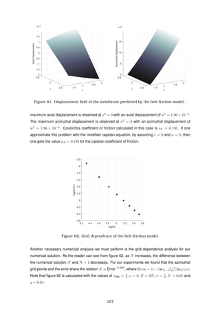
![1.2 1.3 1.4 1.5 1.6 1.7 1.8
δτ
0.05
0.1
0.15
0.2
0.25
0.3
CoefficientofFriction
Capstan
Coulombs
Figure 63: Coefficient of friction relative to δτ = τmax/τ0.
Figure 63 is calculated with the values δτ ∈ {0, 1
20 , 2
20 , 3
20 , 4
20 , 5
20 , 6
20 , 7
20 , 8
20 , 9
20 }, c = 0, E = 103
,
ν = 1
4 , V = 0.01 and = 0.01. It shows that as the tension ratio increases, the coefficient of friction
also increases. This is intuitive as the maximum applied-tension increases, the coefficient of friction
must increases to maintain a constant speed, and thus, a strong correlation between the tension
ratio, and both capstan and Coulomb’s coefficient of friction.
0 0.05 0.1 0.15 0.2 0.25
c
0.175
0.18
0.185
0.19
0.195
0.2
0.205
0.21
0.215
CoefficientofFriction
Capstan (max)
Capstan (min)
Coulombs
Figure 64: Coefficient of friction relative to c.
Now, let us examine what effect varying Gaussian curvature, K = F 1
[II]1F 2
[II]2, has on the coefficient
of friction. Note that K is a function of x1
, and thus, it varies across the contact surface. Let x1
≈ 0
or x1
≈ 1, then, if c ≈ 0, then K ≈ 0 and, if c ≈ 1, then K ≈ (1 − c)−1
. This implies that there exists
a positive correlation between c and K, i.e. as c increases so does K. Thus, we investigate how c
related to νF . Figure 64 is calculated with the values δτ = 3
2 , c ∈ {0, 1
40 , 2
40 , 3
40 , 4
40 , 5
40 , 6
40 , 7
40 , 8
40 , 9
40 },
E = 103
, ν = 1
4 , V = 0.01 and = 0.01. Figures 64 shows that as c increases (i.e. Gaussian cur-
vature increases) coefficient of friction decreases and there exists an optimum value of c where the
158](https://image.slidesharecdn.com/a24f3df3-5be8-40a0-a0ff-910a71f94372-170108131508/85/PhDKJayawardana-164-320.jpg)
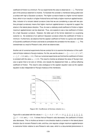
![the literature [96]. Thus, one expects to see coefficient of friction to decrease as Poisson’s ratio
increases. Furthermore, the figure also shows that when Poisson’s ratio is zero, the capstan coeffi-
cient of friction it is an underestimate of Coulomb’s coefficient of friction.
0 0.02 0.04 0.06 0.08 0.1
v
0.1951
0.19512
0.19514
0.19516
0.19518
0.1952
0.19522
0.19524
0.19526
0.19528
CoefficientofFriction
Capstan
Coulombs
Figure 66: Coefficient of friction relative to V .
Figure 66 is calculated with the values δτ = 3
2 , c = 0, E = 103
, ν = 1
4 , V ∈ {0, 1
100 , 2
100 , 3
10 , 4
10 , 5
10 , 6
10 ,
7
10 , 8
10 , 9
10 , 1} and = 0.01. It shows that as the speed in which the membrane is being pulled
increases, the coefficient of friction also increases. This may seems counter intuitive, but consider
following fact: a centripetal force is required to keep a body on a curved path, and higher the
speed of the body is then higher ( higher in magnitude) the centripetal force is required to keep the
body in the given curved orbit. Thus, for our case a higher speed implies a lower normal reaction
force, which in turn implies a lower frictional force. This means that one requires a lower maximum
applied-tension, and this is also a result implied by the modified capstan equation. Thus, as the
speed in which the membrane is being pulled increases, the coefficient of friction also increases.
0 0.01 0.02 0.03 0.04 0.05
ρ
0
0.05
0.1
0.15
0.2
0.25
0.3
CoefficientofFriction
Capstan
Coulombs
Figure 67: Coefficient of friction relative to ρ.
160](https://image.slidesharecdn.com/a24f3df3-5be8-40a0-a0ff-910a71f94372-170108131508/85/PhDKJayawardana-166-320.jpg)
![Figure 67 is calculated with the values of δτ = 3
2 , c = 0, E = 103
, ν = 1
4 , V = 0.01 and ∈ {0, 1
10
2
10 ,
3
10 , 4
10 , 5
10 , 6
10 , 7
10 , 8
10 , 9
10 , 1}. This shows as the mass density (with respect to the volume) of the
membrane increases, both capstan and Coulomb’s coefficient of friction decreases significantly.
Out of all the numerical experiments this has is the most significant result as for a relatively small
decrease in mass density leads to such an enormous increase in the coefficient of friction, for
both capstan and Coulomb’s. Thus, for a given membrane mass density appears to be the most
significant variable that affects the value of the coefficient of friction.
6.4 Experimental Data: June 2015 Trial
In this section we analyse the data obtained from experiments that we conducted on human sub-
jects based on Cottenden et al. [45], Cottenden et al. [46] and Cottenden et al.’s [48] experimental
methodology. We recruit 10 subjects, 5 males and 5 females, all between the ages of 18 to 60, and
we obtained the approval to do so from the UCL Research Ethics Committee: UCL Ethics Project
ID number 5876/001. Experimentee data is found in table 2 if the reader wishes to reproduce any
results, where BMI is the body mass index, Radius is the radius of the mid upper arm and δl is a
measure of how flaccid subject’s tissue is. For more comprehensive set of raw data please consult
Dr N. Ovenden of UCL at n.ovenden@ucl.ac.uk.
Subject Gender Age (Years) BMI Radius (cm) δl
F19 Female 19 21.0 3.98 0.994
F34 Female 34 22.0 4.22 0.991
F40 Female 40 23.4 3.82 1.01
F53 Female 53 27.3 4.54 1.02
F60 Female 60 22.5 4.46 1.02
M18 Male 18 17.5 3.50 0.98
M23 Male 23 24.7 4.77 1.04
M25 Male 25 22.6 4.22 1.01
M26 Male 26 22.8 4.50 0.988
M54 Male 54 26.2 5.09 1.00
Table 2: Experimentee data 2015.
Our experimental configuration is as follows. We first record subject’s gender, age, height, weight
and the dimension of their upper arm. Then, we place their upper arm horizontally, bicep facing
upwards, on an armrest that is designed for subject’s comfortability during the experiments. The
armrest acts also as a restraint to limit subject’s movement, and thus, to reduce the chance of
skewed data. Then, we place a fabric (a nonwoven fabric) over their bicep and attach one end to
the tensometer (Dia-Stron MTT170 provided by Dr S. Falloon of UCL). The dimensions of the fab-
ric is 4cm×50cm, and from our measurements, the fabric has an approximate thickness of 0.5mm
and an approximate mass of 0.6g. It is given to us that the fabric is 95% polypropylene and 5%
161](https://image.slidesharecdn.com/a24f3df3-5be8-40a0-a0ff-910a71f94372-170108131508/85/PhDKJayawardana-167-320.jpg)
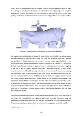
![One of the biggest problems we faced with these experiments is the difficulty in obtaining accurate
data. The contributing factors that reduce the reliability of data are: (i) The markers that we use must
to be large enough so that there are visible in the .stl files, which are generated by the 3D scanner,
but this inherently introduces a very large error in the region of 2mm×4mm×4mm, as every time
we select a marker, we cannot guarantee on the exact location on the marker that we are selecting.
This margin of error is relatively high as most marker displacements from the unstrained position is
less than 4mm; (ii) Due to the obscure angle of the 3D scanner some of the markers cannot be iden-
tified on the .stl files. Very often the unidentifiable markers are A1 to A3; (iii) The tensometer uses
Windows 98 operating system to function, and thus, it is often prone to crashes, leading to much
data loss; (iv) Subjects’ inability remain stationary during the course of the experiment have skewed
the data significantly. Note that duration of each experimental run is approximately 3 minutes. Even
with constant breaks no subject is capable of staying perfectly stationary for 3 minutes at a time for
at least 12 times; (v) Stick and slip behaviour. The error introduced by selecting marker positions
can be minimised if we use much larger masses, but with larger masses we often observe stick and
slip behaviour (see section 13.2 of Kikuchi and Oden [102] for more on stick and slip behaviour)
with an approximate frequency of 1Hz. This is huge problem and it is mostly observed in younger
subjects, especially in F19, M18 and M23. In fact, for F19 this phenomenon is observed for the
lowest of masses. The reason why stick and slip phenomenon is a problem is that the 3D scanner
takes an instant scan, i.e. a snapshot like an ordinary camera, and thus, if the snapshot is taken
in the stick period, then the scanner can record the true deformation, but, if the snap shot is taken
during the slip period, then the scanner cannot record the true deformation as the skin of the subject
is relaxed and it is now in between a state of full and zero deformation; (vi) The perspiration of the
subject during the experiment. In the literature, hydration of the skin shown to significantly increase
the coefficient of friction between skin and fabrics [55, 170]. During the course of the experiment
the level of a subject’s perspiration may change and this may significantly skew the data. In our
experiments heavy perspiration is observed in the subjects M23 and M26; (vii) We cannot measure
the physical and elastic properties (Young’s modulus, Poisson’s ratio, internal biological structure
and dimensions) of subject’ upper arm. Thus, we are deprived of vital data that are required for a
three-dimensional numerical model.
Table 3 shows the tension ratio, δτ = Tmax/T0, for each subject with respect to each applied mass,
where Tmax are the tensometer readings, T0 = Mass × g are the weight of the applied mass and
g = 9.81 is the acceleration due to gravity. Note that the tensometer data of F34 for 60g, M25 for
140g and M54 for 40g are corrupted.
Cottenden et al. [45], Cottenden et al. [46] and Cottenden et al.’s [48] experimental methodology
implies that belt-friction modes, capstan equation in particular, can be used to accurately calculate
the coefficient of friction between in-vivo skin and fabrics. However, belt-friction models assume that
the foundation is rigid, and thus, it is now unsuitable to apply a belt-friction model to calculate the
coefficient friction as now the foundation is not rigid, i.e. as subjects’ tissue is elastic. If belt-friction
models are applicable to model coefficient of friction as the authors assert, then we expect to see a
163](https://image.slidesharecdn.com/a24f3df3-5be8-40a0-a0ff-910a71f94372-170108131508/85/PhDKJayawardana-169-320.jpg)
![Subject
δτ
40g 60g 80g 100g 120g 140g
F19 2.19 1.70 1.52 1.92 1.88 1.86
F34 2.08 · · · 1.93 1.89 1.83 1.83
F40 1.99 1.96 1.92 1.89 1.88 1.79
F53 2.13 2.31 2.23 2.15 1.84 1.70
F60 2.29 2.20 2.06 1.99 1.96 1.95
M18 1.99 1.90 1.88 1.84 1.68 1.76
M23 2.46 2.28 2.24 2.19 2.33 1.99
M25 2.14 1.98 1.81 1.80 1.98 · · ·
M26 2.41 2.31 2.26 2.18 2.31 1.99
M54 · · · 2.12 2.03 1.77 1.91 1.96
Table 3: Experimental data 2015.
40 60 80 100 120 140
Mass (g)
1.5
1.6
1.7
1.8
1.9
2
2.1
2.2
2.3
2.4
2.5
δτ
Mean
40 60 80 100 120 140
Mass (g)
1.85
1.9
1.95
2
2.05
2.1
2.15
δτ
Linear Regression (R2
=0.899)
Figure 69: Tension ratio against applied mass (in grams).
constant relationship between tension ratios and the applied masses. But, if one consult figure 69,
one can see the how the tension ratio vary with the applied mass. In fact, if one calculates the mean
coefficients friction between the fabric and subjects’ skin, a non-constant relationship between the
coefficients of friction and the applied mass is evident (see figure 70). This offers clear evidence
that belt-friction models are not suitable for measuring the coefficient of friction when the foundation
is no longer rigid. Note that the mean values of Coulomb’s coefficient of friction is calculated with
the belt-friction model for E = 103
, ν = 1
4 and a terminating error of 10−8
. Also, mean values cap-
stan coefficient of friction is calculated with the extended capstan equation (82) with Matlab fsolve
function.
Cottenden et al. [45], Cottenden et al. [47] and Karavokyros [100] do acknowledge this problem
and assert that the there exists a c0 such that Tmax = c0 + T0 exp(µF θ0), where c0 is the inter-
164](https://image.slidesharecdn.com/a24f3df3-5be8-40a0-a0ff-910a71f94372-170108131508/85/PhDKJayawardana-170-320.jpg)
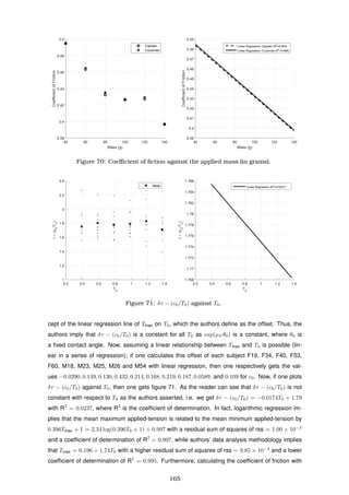
![authors’ linear regression method leads to a positive correlation between the coefficient of friction
and the radius of subjects’ upper arm, which is not a desirable result and we explain why this is
so in later analysis. Now, this is direct evidence that one must not use linear regression models to
model friction between fabrics and in-vivo skin. Note that all regression results are calculated with
Regression Tools at Xuru’s Website [214].
The above numerical and regression analysis motivates one to make the following hypothesis:
Hypothesis 4. Consider a rectangular membrane over a rough elastic prism whose un-
strained contact region parameterised by the map (x, f(θ), g(θ))E, where f(·) and g(·) are
C1
([θ0, θmax]) 2π-periodic functions, |x| ≤ ∞, and the contact interval [θ0, θmax] is chosen such
that g f − f g > 0, ∀ x2
∈ [θ0, θmax]. If Tmax is the maximum applied-tension at θmax and T0
is the minimum applied-tension at θ0, then there exists a regression curve Y (·) of the form
εTmax + ξ = Y (εT0 + ξ), such that Y (ξ) is positive and invariant with respect to the quantity
r0 = arctan
g (θ0)
f (θ0)
− arctan
g (θmax)
f (θmax)
−1 θmax
θ0
(f )2
+ (g )2
1
2
dθ ,
where the normalising constant ε is chosen such that ε ≤ 1/max(Tmax) and the translating
constant ξ is chosen such that Y (ξ) is not singular. Furthermore, given such a regression
curve Y (·), the coefficient of friction µF has the following relation,
µF = arctan
g (θ0)
f (θ0)
− arctan
g (θmax)
f (θmax)
−1
log (Y (ξ)) ,
and, in particular, µF is independent of r0.
Given a rectangular membrane with a zero-Poisson’s ratio over a rigid cylinder, in our experimental
configuration the solution for the tension across the membrane takes the form described by equation
(82) (see Section 6.3 for more detail). Thus, the regression curve of Tmax on T0 can be expressed
as Tmax = c0 + c1T0, where
c0 = lh
V 2
r0
1 − exp
1
2
πµF + lhg
1 − µ2
F
1 + µ2
F
+
2µF
1 + µ2
F
exp
1
2
πµF ,
c1 = exp
1
2
πµF ,
and where l is the width and h is the thickness of the membrane, and thus, µF = 2π−1
log(c1).
However, if one consider a membrane of nonzero Poisson’s ratio or an elastic prism, then this lin-
ear regression line of Tmax on T0 will no longer hold. Thus, hypothesis 4 is a simple extension of
this observation with the use of theorem 1. Note that Doonmez and Marmarali [59] used multiple
regression analysis to study the coefficient of friction, and thus, further justifying the necessity for
hypothesis 4.
Due to the finite deformation of both the membrane and the foundation under stress we predict that
the regression curve has the form Y (εT0 + 1) = a + b(εT0 + 1) + c log(εT0 + 1), where a, b and c are
constants to be determined by a given experiment and the log(·) term is implied by the true strain
(for more on true strain please consult Rees [167]). Thus, in our experimental configuration we
have µF = 2π−1
log(b + c). Unfortunately, our experimental data is not comprehensive enough and
166](https://image.slidesharecdn.com/a24f3df3-5be8-40a0-a0ff-910a71f94372-170108131508/85/PhDKJayawardana-172-320.jpg)
![our understanding in regression analysis is not extensive enough to test this hypothesis or more
generally to test hypothesis 4.
As we cannot calculate the coefficient of friction with a good degree of accuracy, let us use the
tension ratio, δτ, to find some useful information regarding the frictional interaction between in-vivo
skin and fabrics. Note that figure 63 from our numerical analysis implies that there exists a strong
positive correlation between the tension ratio and the coefficient of friction. Thus, the tension ratio
from our experiments maybe used to infer the nature of the coefficient of friction between subjects’
skin and the fabric.
10 20 30 40 50 60
Age (years)
1.8
1.85
1.9
1.95
2
2.05
2.1
2.15
2.2
2.25
δτ
Mean
Regression (R2
=0.0512)
Figure 72: Coefficient of fiction against the age (in years).
Figure 72 shows the tension ratio against subjects’ age, where the linear regression line is δτ =
0.00117 × Age + 1.96 and the age is in years (R2
= 0.0512). As the reader can see there is no ob-
vious relationship between the age of the subject and the tension ratio. In fact, the highest tension
ratios are observed in M23 and M26 (two of the youngest subjects) who were excessively perspiring
during the course of the experiments.
Figure 73 shows the tension ratio against the body mass index (BMI), where the linear regression
line is δτ = 0.0169 × BMI + 1.61 (R2
= 0.0961). Note that the BMI is calculated with the use of the
NHS BMI calculator [199]. As the reader can see that there is a vague positive correlation between
the BMI and the tension ratio. However, this does neither imply nor does not imply that those who
are with a higher BMI have a greater risk of skin abrasion, i.e correlation does not imply causation
[6]. The reason we observe this correlation is because that those who have a higher BMI tend to
have a greater fat content, i.e. higher volume of flaccid tissue. Thus, during the experiments a
higher tension needs to be applied to the fabric as the as a portion of the tension is expended on
deforming the flaccid tissue of the subject. If this higher tension is fed in to a belt-friction model, then
what one gets in return is a higher coefficient of friction. This is a perfect example of garbage in,
garbage out [177], where a logical numerical model outputting nonsensical gibberish due to flawed
167](https://image.slidesharecdn.com/a24f3df3-5be8-40a0-a0ff-910a71f94372-170108131508/85/PhDKJayawardana-173-320.jpg)
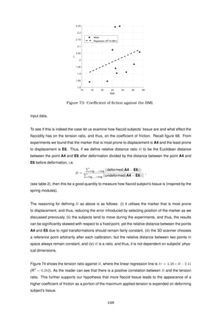
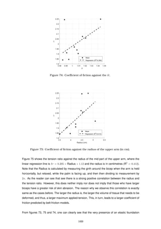
![leads to a nonlinear relationship between T0 and Tmax, which in turn can significantly skew ones
experimental results if one uses a belt-friction model to calculate the coefficient of friction.
6.4.1 Remark
A possible technique that maybe used to measure the coefficient of friction of human skin is by a
method proposed by Asserin et al. [9]. The authors construct a device that is capable of mea-
suring the coefficient of friction between a reference material and in-vivo human skin. They state
that the device is accurate enough to discern the arithmetic mean of roughness between the values
0.4µm–50µm, where µm is the units for micrometers. The in-vivo experiments are conducted on
three human subjects. They is all female with each having the ages 20, 42 and 50. The authors
calculate the coefficient of friction of the 42 year old female’s lower arm which is 0.7, but the coeffi-
cient of friction with respect to what reference material is not specified. With their device the authors
hope to investigate the change in texture of the skin due to the application of cosmetic products.
6.5 Shell-Membranes Supported by Elastic Foundations with Static
Friction
In this section we derive a shell-membrane model to describe the behaviour of overlying membranes
on elastic foundations subjected to static friction. Recall our shell model with friction from chapter4,
but now assume that the thickness of the shell is so thin and the bending moments are so small
that the overlying body can further be approximated by a shell-membrane. Thus, we obtain:
Corollary 5. Let Ω ⊂ R3
be a connected open bounded domain that satisfies the segment
condition with a uniform-C1
(R3
; R2
) boundary ∂Ω such that ω, ∂Ω0 ⊂ ∂Ω, where ¯ω ∩ ¯∂Ω0 = Ø
with meas(∂Ω0; R2
) > 0, and let ω ⊂ R2
be a connected open bounded plane that satisfies
the segment condition with a uniform-C1
(R2
; R) boundary ∂ω. Let ¯X ∈ C1
(¯Ω; E3
) be a diffeo-
morphism and be σ ∈ C2
(¯ω; E3
) be injective an immersion. Let f ∈ L2
(Ω), f0 ∈ L2
(ω) and
τ0 ∈ L2
(∂ω). Then there exists a unique field u ∈ VM (ω, Ω) such that u is the solution to the
minimisation problem
J(u) = min
v∈VM (ω,Ω)
J(v) ,
where
VM (ω, Ω) = {v ∈ H1
(Ω) | v|ω ∈ H1
(ω)×H1
(ω)×L2
(ω), v|∂Ω0
= 0, 2νF v3
+ (vαvα
)
1
2 |ω ≤ 0 a.e.} ,
J(u) =
Ω
1
2
Aijkl
Eij(u)Ekl(u) − fi
ui dΩ
+ h
ω
1
2
Bαβγδ
αβ(u) γδ(u) − fi
0ui dω − h
∂ω
τα
0 uα d(∂ω) ,
h is the thickness of the shell-membrane and νF is the coefficient of friction between the
foundation and the shell-membrane.
Proof. Follows from theorem 4 for the h2
ργ
α(u)ρα
γ (u) γ
α(u) α
γ (u) case and the results on
shell-membranes from chapters 4 and 5 of Ciarlet [38].
170](https://image.slidesharecdn.com/a24f3df3-5be8-40a0-a0ff-910a71f94372-170108131508/85/PhDKJayawardana-176-320.jpg)
![6.6 Numerical Analysis
To conduct numerical experiments assume a shell-membrane with a thickness h, supported by
an elastic foundation, where the unstrained configuration of the foundation is an annular cylin-
drical which is characterised by the diffeomorphism ¯X(x, θ, r) = (x, r sin(θ), r cos(θ))E, where
(x1
, x2
, x3
) = (x, θ, r), x ∈ (−L, L), θ ∈ (−π, π] and r ∈ (a0, a), and assume that the contact
region is defined by x ∈ (− , ), θ ∈ (−1
2 π, 0), where 0 < < L. Let the sufficiently smooth
field u = (u1
(x, θ, r), u2
(x, θ, r), u3
(x, θ, r)) be the displacement field of the foundation. With some
calculations one finds that the metric tensor is g = diag(1, r2
, 1) and the covariant derivatives are
¯1u1
= ∂1u1
, ¯1u2
= ∂1u2
, ¯1u3
= ∂1u3
,
¯2u1
= ∂2u1
, ¯2u2
= ∂2u2
+ r−1
u3
, ¯2u3
= ∂2u3
− ru2
,
¯3u1
= ∂3u1
, ¯3u2
= ∂3u2
+ r−1
u2
, ¯3u3
= ∂3u3
.
With further calculations, one can express the governing equations of the foundation as
(¯λ + ¯µ)∂1
( ¯iui
) + ¯µ ¯∆u1
= 0 ,
(¯λ + ¯µ)∂2
( ¯iui
) + ¯µ ¯∆u2
= 0 ,
(¯λ + ¯µ)∂3
( ¯iui
) + ¯µ ¯∆u3
= 0 .
The boundary of the foundation can be decomposed into sub-boundaries as
∂Ω = ¯ω ∪ ∂Ω0 ∪ ∂Ωf ,
ω = {a} × (−
1
2
π, 0) × (− , ) ,
∂Ω0 = {{a0} × (−π, π] × [−L, L]} ∪ {(a0, a] × (−π, π] × {{−L} ∪ {L}}} ,
∂Ωf = {{a} × (−π, π] × (−L, L)} ¯ω .
Thus, one can express the boundary conditions of the foundation as
u|∂Ω0
= 0 (zero-Dirichlet) ,
∂3u1
+ ∂1u3
|∂Ωf
= 0 (zero-Robin) ,
r2
∂3u2
+ ∂2u3
|∂Ωf
= 0 (zero-Robin) ,
¯λ(∂1u1
+ ∂2u2
+ r−1
u3
) + (¯λ + 2¯µ)∂3u3
|∂Ωf
= 0 (zero-Robin) .
Let u|ω = (u1
(x, θ, a), u2
(x, θ, a), u3
(x, θ, a)) be the displacement field of the shell-membrane. With
some calculations, one finds that the first fundamental form tensor is F[I] = diag(1, a2
) and the
covariant derivatives are
1u1
= ∂1u1
, 1u2
= ∂1u2
,
2u1
= ∂2u1
, 2u2
= ∂2u2
.
With further calculations (see Section 4.3.3 and considering the case h2
ργ
α(u)ρα
γ (u) γ
α(u) α
γ (u)),
one can express the governing equations of the shell-membrane as:
171](https://image.slidesharecdn.com/a24f3df3-5be8-40a0-a0ff-910a71f94372-170108131508/85/PhDKJayawardana-177-320.jpg)
![If [2νF u3
+ (u1
u1
+ r2
u2
u2
)
1
2 ]|ω < 0, then
(Λ − µ)∂1
( αuα
) + µ∆u1
+
1
a
(Λ − 2µ)∂1
u3
−
1
h
Tr(T1
3 (u)) = 0 ,
(Λ − µ)∂2
( αuα
) + µ∆u2
+
1
a
Λ∂2
u3
−
1
h
Tr(T2
3 (u)) = 0 ,
(Λ − 2µ)∂1u1
+ Λ ∂2u2
+
1
a
u3
+
a
h
Tr(T3
3 (u)) = 0 ,
where Λ = 2λµ(λ + 2µ)−1
;
If [2νF u3
+ (u1
u1
+ r2
u2
u2
)
1
2 ]|ω = 0, then
(Λ − µ)∂1
( αuα
) + µ∆u1
−
(Λ − 2µ)
2aνF
∂1
(u1
u1
+a2
u2
u2
)
1
2 −
1
h
Tr(T1
3 (u)) −
(Λ − µ)
4aν2
F
u1
−
(¯λ + ¯µ)
4hν2
F
u1
+
1
2νF
u1
(u1u1 +a2u2u2)
1
2
(Λ − 2µ)∂1u1
+ Λ∂2u2
+
a
h
¯λ(∂1u1
+ ∂2u2
) + (¯λ + 2¯µ)∂3u3
= 0 ,
(Λ − µ)∂2
( αuα
) + µ∆u2
−
Λ
2aνF
∂2
(u1
u1
+a2
u2
u2
)
1
2 −
1
h
Tr(T2
3 (u)) −
(Λ − µ)
4aν2
F
u2
−
(¯λ + ¯µ)
4hν2
F
u2
+
1
2νF
u2
(u1u1 +a2u2u2)
1
2
(Λ − 2µ)∂1u1
+ Λ∂2u2
+
a
h
¯λ(∂1u1
+ ∂2u2
) + (¯λ + 2¯µ)∂3u3
= 0 .
The boundary of the shell-membrane can be decomposed into sub-boundaries as
∂ω = ∂ωT0
∪ ∂ωTmax
∪ ∂ωf ,
∂ωT0
= [− , ] × {−
1
2
π} ,
∂ωTmax
= [− , ] × {0} ,
∂ωf = {{− } ∪ { }} ∪ (−
1
2
π, 0) .
Thus, one can express the boundary conditions of the shell-membranes as
(Λ − 2µ)∂1u1
+ Λ(∂2u2
+ a−1
u3
) |∂ωT0
= τ0 (traction) ,
(Λ − 2µ)∂1u1
+ Λ(∂2u2
+ a−1
u3
) |∂ωTmax
= τmax (traction) ,
Λ∂1u1
+ (Λ − 2µ)(∂2u2
+ a−1
u3
) |∂ωf
= 0 (zero-Robin) ,
∂2u1
+ a2
∂1u2
|∂ωf
= 0 (zero-Robin) .
To conduct numerical experiments we employ the second-order-accurate finite-difference method in
conjunction with Newton’s method for nonlinear systems as in Section 2.6. Another issue we must
tackle is the discretisation of the domain. As we are dealing with curvilinear coordinates, there is
a inherit grid dependence. To be precise, it is approximately r∆x2
≤ ∆x1
and r∆x2
≤ ∆x2
, for all
a0 ≤ r ≤ a, where ∆xj
is a small increment in xj
direction. For our purposes we use ∆x2
= 1
N−1
and r = a, where N = 250. Finally, we must define a terminating condition. For this we choose to
terminate our iterating process given that the condition |1 − ||um||−1
2 ||um+1|| 2 | < 10−10
is satisfied.
We model a stiff shell-membrane on a relatively flaccid foundation with a large coefficient of friction.
To do so, we keep the values νF = 1, h = 0.001, a = 1, = 1
4 , L = 1
2 , E = 103
, ν = 1
4 , ¯ν = 0, τ0 = 1
and τmax = 2 fixed for all experiments.
172](https://image.slidesharecdn.com/a24f3df3-5be8-40a0-a0ff-910a71f94372-170108131508/85/PhDKJayawardana-178-320.jpg)
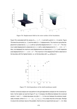
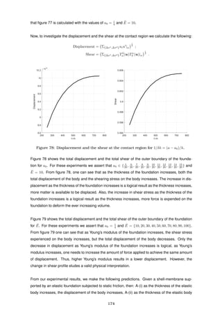

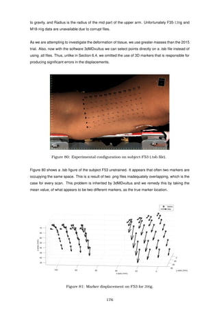
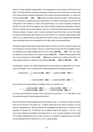
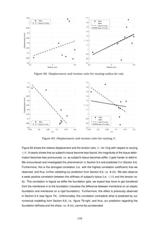
![6.7.1 Remark
A possible technique that maybe used to measure the elastic properties of subject’s tissue, to be
use in our numerical models, is the shearwave dispersion ultrasound vibrometry (SDUV). This is
an ultrasound based method that is used in measuring the shear elasticity and viscosity in various
types of soft tissues with the use of dispersion of shear wave velocities, which arise from the inherent
viscoelastic nature of soft tissue. Urban et al. [202] use SDUV in both ex-vivo (exorcised muscle
samples of porcine and bovine) and in-vivo (a liver and a heart of a porcine) tissues. The authors
state that SDUV gave high temporal and spatial resolution material property measurements of soft
tissue that can be integrated with B-mode imaging (medical ultrasound that displays the acoustic
impedance of a two-dimensional cross-section of tissue) to provide a new tool for clinicians to use
for diagnosis and monitoring of therapies.
6.8 Conclusions
In this chapter we investigated aspects of mathematically modelling skin damage due to friction. In
Section 6.2 we derived a belt-friction model, for a true-membrane over a non-hyperbolic rigid obsta-
cle with a positive mean-curvature, with the use of Kikuchi and Oden’s [102] model for Coulombs
law of static friction for the slip case. This belt-friction model is derived with a very hypothetical
approach. Thus, we are unable to conduct finer analysis, including the existence of solutions, due
to the fact that it is not possible to express the governing equations in a variational form. Therefore,
we remind the reader that what we derived is not a mathematical theory. By conducting numerical
experiments, in Section 6.3, we found that (given that we keep all other variables fixed): (i) there
exists a strong positive correlation between the maximum applied-tension and the coefficient of
friction, (ii) there exists an initial negative correlation between the Gaussian curvature of the rigid
foundation and the coefficient of friction, and there exists an optimum Gaussian curvature where the
coefficient of friction is a minimum, (iii) there exists a negative correlation between Poisson’s ratio
of the membrane and the coefficient of friction, (iv) there exists a negative correlation between the
speed in which the membrane is being pulled and the coefficient of friction, (v) there exists a posi-
tive correlation between the mass density of the membrane and the coefficient of friction, where the
mass density of the membrane is responsible for significantly increasing the coefficient of friction
relative to other variables, and (vi) the coefficient of friction is not affected by Young’s modulus of the
membrane, which coincide with the capstan equation as it is also independent of Young’s modulus
of the membrane, given that Young’s modulus is neither zero nor infinite. All the results we found
are intuitive, but the existence of an optimum Gaussian curvature where the coefficient of friction is
a minimum is a surprising result.
In Section 6.4, with experiments conducted on human subjects and with elementary regression
analysis, we show that it is unwise to use belt-friction models to calculate the friction between
in-vivo skin and fabrics as the existence of an elastic foundation can significantly influence one’s
experimental results. We found that, if one uses a belt-friction model to calculate the coefficient of
friction between in-vivo skin and fabrics, then there exists a weak, but a positive correlation between
179](https://image.slidesharecdn.com/a24f3df3-5be8-40a0-a0ff-910a71f94372-170108131508/85/PhDKJayawardana-185-320.jpg)
![7 Conclusions
In this thesis we presented a general theory for static linearly elastic isotropic shells supported by
static linearly elastic isotropic foundations, for both the bonded and frictionally coupled cases in
curvilinear coordinates.
We began in chapter 1 where we introduced the critical definitions, the fundamental theorems and
the most notable applications relating to the study of shell and membrane theory, and contact con-
ditions governing elastic bodies, in particular, friction. There, we critically analysed the existing liter-
ature on the study of thin objects such as films, plates, membranes and shells, and we highlighted
their limitations, flaws and given correct formulations when possible. In particular, we meticulously
documented the erroneous mathematical work of Howell et al. [84] (see Section 1.4), Cottenden
et al. [48] (see Section 1.8), Efrati et al. [60] (see Section 1.9) and Baldelli and Bourdin [16] (see
Section 1.10). The flaws of the given authors’ work are revealed by a combination of correct mathe-
matical proofs and or counterexamples. Furthermore, we offered corrections to their work whenever
possible, again with meticulous detail.
In chapter 2 we examined the behaviour of membranes of zero-Poisson’s ratio (or strings) supported
by rigid foundations of positive mean-curvature and zero-Gaussian curvature, where the contact re-
gion is governed by the common friction-law. To be more precise, we extended the capstan equation
to general geometries and gave closed-form solutions for all the cases.
Then, in Section 2.6, we extended Kikuchi and Oden’s [102] model for Coulomb’s law of static
friction to curvilinear coordinates. There, we conducted numerical experiments to see how close
the modified Kikuchi and Oden’s model resembles the modified capstan equation. Our numerical
results imply that the capstan coefficient of friction is an underestimate of Coulomb’s coefficient of
friction, i.e. µF ≤ νF . Also, for a fixed coefficient of friction, as the critical parametric-latitude of the
contact region increases, as the thickness of the body decreases or as Poisson’s ratio of the body
increases, one requires a larger force to debond the body. In addition, Young’s modulus of the body
does not affect the governing equation at the contact region.
The work presented in chapter 2 has real life applications in cable drive devices, particularly in the
field of robotics. Please consult Section 1.6 for more detail.
In chapter 3 we begin the study of shells that are supported by elastic foundations. To begin, we
considered the case where the shell is bonded to the foundation. We derived the equations for the
overlying shell with the mathematical techniques for Koiter’s linear shell theory and linear elasticity
theory in curvilinear coordinates put forward by Ciarlet [38], and a technique that is used in the
derivation of surface Cauchy-Bourne model [89]. Then, we treated the overlying bonded shell as
a boundary form of the elastic foundation, which is analogous to the work of Necas et al. [144],
and we used the mathematical techniques put forward by Ciarlet [38], and Badiale and Serra [13]
181](https://image.slidesharecdn.com/a24f3df3-5be8-40a0-a0ff-910a71f94372-170108131508/85/PhDKJayawardana-187-320.jpg)
![to mathematically, and thus, conclusively, prove the existence and the uniqueness of solutions for
the proposed model. Thus, concluding that what we derived is a mathematical theory.
To check the physical validity of our work we extended Baldelli and Bourdin’s [16] model for stiff
films on elastic foundations to curvilinear coordinates via asymptotic analysis. Then, in Section
3.5, we numerically modelled the displacement field at the contact region with a bonded two-body
elastic problem and compared the solution against our bonded shell model and extend Baldelli and
Bourdin’s model, for a set of variable which Baldelli and Bourdin’s [16] model is mostly accurate for.
Numerical results show that the error between the bonded two-body solution and extend Baldelli
and Bourdin’s model is always several magnitudes greater than the error between the bonded two-
body solution and our bonded shell solution, and this is the case for all the input variables. This
implies that our shell model is far superior model in comparison when approximating contact region
of thin bodies that are bonded to elastic foundations.
To conclude our numerical analysis for the bonded case, in Section 3.7, we modelled the displace-
ment field of the foundation of the bonded two-body elastic problem and compared the solutions
against our bonded shell solutions. Our analysis showed that our bonded shell on an elastic foun-
dation model can approximate two-body elastic model’s foundation with a significant degree of
accuracy given that Young’s modulus of the shell is significantly higher than Young’s modulus of the
foundation. Now, this result coincides with what is documented in the literature [4]. We also observe
other factors can equally affect the accuracy of our bonded shell model, such as Poisson’s ratio and
the thickness of the shell, and the critical parametric-latitude of the contact region. However, one
cannot arbitrarily increase or decrease elastic and geometrical properties (e.g. cannot arbitrarily in-
crease Young’s modulus of the shell in the hope of gaining accuracy), as we often observe optimal
values for elastic and geometric properties where the error is a minimum.
Chapter 3 is the strongest chapter of the thesis as we have a definitive model (classical three-
dimensional elasticity equations) and a relatively pre-existing model (extended Baldelli and Bour-
din’s model) to compare our bonded shell model against to determined the validity of our work.
Also, these types of models have a wide range of applications, particularly in the field of flexible and
stretchable electronics (see Section 1.7), and they may possibly be applied to model gyrification
(see Section 3.8.1).
In chapter 4 we concluded our study on shells that are supported by elastic foundations by assert-
ing that the contact region is governed by a displacement-based friction condition that is analogous
to Coulomb’s law of static friction. We treated this displacement-based frictional condition as a
constraint, which is analogous to the work of Kinderlehrer and Stampacchia [107], and with the
mathematical techniques put forward by Evans [63], and Kinderlehrer and Stampacchia [107], we
mathematically proved the existence and the uniqueness of solutions, and thus, concluding that
what we derived a mathematical theory.
182](https://image.slidesharecdn.com/a24f3df3-5be8-40a0-a0ff-910a71f94372-170108131508/85/PhDKJayawardana-188-320.jpg)
![References
[1] M. Abramowitz, I. A. Stegun, et al. Handbook of mathematical functions, volume 1046. Dover New York,
1965.
[2] A. Acharya. On compatibility conditions for the left cauchy–green deformation field in three dimensions.
Journal of elasticity, 56(2):95–105, 1999.
[3] R. A. Adams and J. J. F. Fournier. Sobolev spaces, volume 140. Academic press, 2003.
[4] L. Aghalovyan and D. Prikazchikov. Asymptotic theory of anisotropic plates and shells. World Scientific,
2015.
[5] S. Agmon, A. Douglis, and L. Nirenberg. Estimates near the boundary for solutions of elliptic partial
differential equations satisfying general boundary conditions ii. Communications on pure and applied
mathematics, 17(1):35–92, 1964.
[6] J. Aldrich. Correlations genuine and spurious in pearson and yule. Statistical science, pages 364–376,
1995.
[7] H. G. Allen. Analysis and Design of Structural Sandwich Panels: The Commonwealth and International
Library: Structures and Solid Body Mechanics Division. Elsevier, 2013.
[8] G. Angelini, G. A. Vena, and C. L. Meneghini. Shoe contact dermatitis. Contact Dermatitis, 6(4):279–
283, 1980.
[9] J. Asserin, H. Zahouani, P. Humbert, V. Couturaud, and D. Mougin. Measurement of the friction coeffi-
cient of the human skin in vivo: quantification of the cutaneous smoothness. Colloids and surfaces B:
Biointerfaces, 19(1):1–12, 2000.
[10] B. Audoly and A. Boudaoud. Buckling of a stiff film bound to a compliant substrate—part i:: Formulation,
linear stability of cylindrical patterns, secondary bifurcations. Journal of the Mechanics and Physics of
Solids, 56(7):2401–2421, 2008.
[11] B. Audoly and A. Boudaoud. Buckling of a stiff film bound to a compliant substrate—part ii:: A global
scenario for the formation of herringbone pattern. Journal of the Mechanics and Physics of Solids,
56(7):2422–2443, 2008.
[12] B. Audoly and A. Boudaoud. Buckling of a stiff film bound to a compliant substrate—part iii:: Herringbone
solutions at large buckling parameter. Journal of the Mechanics and Physics of Solids, 56(7):2444–2458,
2008.
[13] M. Badiale and E. Serra. Semilinear Elliptic Equations for Beginners: Existence Results via the Varia-
tional Approach. Springer Science & Business Media, 2010.
[14] J. H. Baek, Y. K. Kwak, and S. H. Kim. On the frequency bandwidth change of a servo system with a
gear reducer due to backlash and motor input voltage. Archive of Applied Mechanics, 73(5-6):367–376,
2003.
[15] A. A. L. Baldelli. On Fracture of Thin Films: a Variational Approach. PhD thesis, Citeseer, 2013.
[16] A. A. L. Baldelli and B. Bourdin. On the asymptotic derivation of winkler-type energies from 3d elasticity.
Journal of Elasticity, pages 1–27, 2015.
[17] J. M. Ball. Convexity conditions and existence theorems in nonlinear elasticity. Archive for rational
mechanics and Analysis, 63(4):337–403, 1976.
184](https://image.slidesharecdn.com/a24f3df3-5be8-40a0-a0ff-910a71f94372-170108131508/85/PhDKJayawardana-190-320.jpg)
![[18] S. J. Ball, I. E. Brown, and S. H. Scott. A planar 3dof robotic exoskeleton for rehabilitation and assess-
ment. In Engineering in Medicine and Biology Society, 2007. EMBS 2007. 29th Annual International
Conference of the IEEE, pages 4024–4027. IEEE, 2007.
[19] O. Baser and E. I. Konukseven. Theoretical and experimental determination of capstan drive slip error.
Mechanism and Machine Theory, 45(6):815–827, 2010.
[20] R. Basex A., Salvador and A. Dupre. Pseudo-chromidrose plantaire. Bull Soc Franc Dermatol Syph,
69:489–490, 1962.
[21] S. Behzadipour and A. Khajepour. Cable-based robot manipulators with translational degrees of free-
dom. INTECH Open Access Publisher, 2006.
[22] G. Bennett, C. Dealey, J. Posnett, et al. The cost of pressure ulcers in the uk. Age and ageing, 33(3):230–
235, 2004.
[23] R. W. Berg. Etiologic factors in diaper dermatitis: a model for development of improved diapers. Pedia-
trician, 14:27, 1987.
[24] W. F. Bergfeld and J. S. Taylor. Trauma, sports, and the skin. American journal of industrial medicine,
8(4-5):403–413, 1985.
[25] N. Bergstrom. Treatment of Pressure Ulcers. AHCPR pub. Diane Publishing Company, 1994.
[26] S. R. Bodner, J. Singer, A. Solan, and Z. Hashin. Theoretical and Applied Mechanics 1992. Elsevier
Science, 2012.
[27] E. Bonderover and S. Wagner. A woven inverter circuit for e-textile applications. Electron Device Letters,
IEEE, 25(5):295–297, 2004.
[28] F. P. Bowden and D. Tabor. The friction and lubrication of solids, volume 2. Wiley Online Library, 1964.
[29] A. Brooks, G. Dickins, A. Zelinsky, J. Kieffer, and S. Abdallah. A high-performance camera platform for
real-time active vision. In Field and Service Robotics, pages 527–532. Springer, 1998.
[30] R. Burden, J. Faires, and A. Burden. Numerical analysis. Nelson Education, 2015.
[31] L. T. Campos, J. T. Oden, and N. Kikuchi. A numerical analysis of a class of contact problems with friction
in elastostatics. Computer Methods in Applied Mechanics and Engineering, 34(1):821–845, 1982.
[32] M. C. Carrozza, G. Cappiello, S. Micera, B. B. Edin, L. Beccai, and C. Cipriani. Design of a cybernetic
hand for perception and action. Biological cybernetics, 95(6):629–644, 2006.
[33] M. C. Choi, Y. Kim, and C. S. Ha. Polymers for flexible displays: From material selection to device
applications. Progress in Polymer Science, 33(6):581–630, 2008.
[34] R. Christensen. Log-linear models and logistic regression. Springer Science & Business Media, 2006.
[35] J. U. Chu, D. H. Jeong, I. Youn, K. Choi, and Y. J. Lee. Myoelectric hand prosthesis with novel
adaptive grasping and self-locking. International Journal of Precision Engineering and Manufacturing,
12(6):1095–1103, 2011.
[36] P. G. Ciarlet. Mathematical elasticity. vol. i, volume 20 of studies in mathematics and its applications,
1988.
[37] P. G. Ciarlet. Theory of Plates. Mathematical Elasticity. Elsevier Science, 1997.
[38] P. G. Ciarlet. Theory of Shells. Mathematical Elasticity. Elsevier Science, 2000.
[39] P. G. Ciarlet. An introduction to differential geometry with applications to elasticity. Journal of Elasticity,
78(1-3):1–215, 2005.
185](https://image.slidesharecdn.com/a24f3df3-5be8-40a0-a0ff-910a71f94372-170108131508/85/PhDKJayawardana-191-320.jpg)
![[40] P. G. Ciarlet and C. Mardare. An introduction to shell theory. Differential Geometry: Theory and Appli-
cations, 9:94–184, 2008.
[41] S. K. Clark. Mechanics of pneumatic tires. US Department of Transportation, National Highway Traffic
Safety Administration, 1981.
[42] M. Controzzi, C. Cipriani, and M. C. Carrozza. Miniaturized non-back-drivable mechanism for robotic
applications. Mechanism and Machine Theory, 45(10):1395–1406, 2010.
[43] S. M. Copperman. Two new causes of alopecia. JAMA, 252(24):3367–3367, 1984.
[44] T. A. Cortese, K. Fukuyama, W. Epstein, and M. B. Sulzberger. Treatment of friction blisters: an experi-
mental study. Archives of dermatology, 97(6):717–721, 1968.
[45] A. M. Cottenden, D. J. Cottenden, S. Karavokiros, and W. K. R. Wong. Development and experimental
validation of a mathematical model for friction between fabrics and a volar forearm phantom. Proceed-
ings of the Institution of Mechanical Engineers, Part H: Journal of Engineering in Medicine, 222(7):1097–
1106, 2008.
[46] A. M. Cottenden, W. K. Wong, D. J. Cottenden, and A. Farbrot. Development and validation of a new
method for measuring friction between skin and nonwoven materials. Proceedings of the Institution of
Mechanical Engineers, Part H: Journal of Engineering in Medicine, 222(5):791–803, 2008.
[47] D. J. Cottenden. A multiscale analysis of frictional interaction between human skin and nonwoven fabrics.
PhD thesis, UCL (University College London), 2011.
[48] D. J. Cottenden and A. M. Cottenden. An analytical model of the motion of a conformable sheet over a
general convex surface in the presence of frictional coupling. The Quarterly Journal of Mechanics and
Applied Mathematics, page hbp012, 2009.
[49] P. S. Cowen et al. Juvenile plantar dermatosis in an adult. British Journal of Dermatology, 104(5):599–
599, 1981.
[50] G. Crawford. Flexible flat panel displays. John Wiley & Sons, 2005.
[51] J. Crissey and J. Peachy. Calcaneal petechiae. Arch Dermatol, 83:501, 1961.
[52] S. Cuenot, C. Fr´etigny, S. Demoustier-Champagne, and Be. Nysten. Surface tension effect on the
mechanical properties of nanomaterials measured by atomic force microscopy. Physical Review B,
69(16):165410, 2004.
[53] A. S. Demidov. Generalized functions in mathematical physics: main ideas and concepts, volume 237.
Nova Publishers, 2001.
[54] L. Demkowicz and J. T. Oden. On some existence and uniqueness results in contact problems with
nonlocal friction. Nonlinear Analysis: Theory, Methods & Applications, 6(10):1075–1093, 1982.
[55] S. Derler and L. C. Gerhardt. Tribology of skin: review and analysis of experimental results for the friction
coefficient of human skin. Tribology Letters, 45(1):1–27, 2012.
[56] D. A. Dillard, J. A. Hinkley, W. S. Johnson, and T. L. St. Clair. Spiral tunneling cracks induced by
environmental stress cracking in larcTM
-tpi adhesives. The Journal of Adhesion, 44(1-2):51–67, 1994.
[57] H. Ding, W. Chen, and L. Zhang. Elasticity of transversely isotropic materials, volume 126. Springer
Science & Business Media, 2006.
[58] M. P. do Carmo. Differential Geometry of Curves and Surfaces. Pearson Education Taiwan Limited,
2009.
186](https://image.slidesharecdn.com/a24f3df3-5be8-40a0-a0ff-910a71f94372-170108131508/85/PhDKJayawardana-192-320.jpg)
![[59] S. D¨oonmez and A. Marmarali. A model for predicting a yarn’s knittability. Textile research journal,
74(12):1049–1054, 2004.
[60] E. Efrati, E. Sharon, and R. Kupferman. Elastic theory of unconstrained non-euclidean plates. Journal
of the Mechanics and Physics of Solids, 57(4):762–775, 2009.
[61] P. H. Ely. Balance beam alopecia. Archives of dermatology, 114(6):968, 1978.
[62] E. Epstein. Granuloma fissuratum of the ears. Archives of dermatology, 91(6):621–622, 1965.
[63] L. C. Evans. Partial Differential Equations. Graduate studies in mathematics. American Mathematical
Society, 2010.
[64] M. A. Farage, K. W. Miller, E. Berardesca, and H. I. Maibach. Incontinence in the aged: contact dermatitis
and other cutaneous consequences. Contact Dermatitis, 57(4):211–217, 2007.
[65] S. R. Forrest. The path to ubiquitous and low-cost organic electronic appliances on plastic. Nature,
428(6986):911–918, 2004.
[66] G. Friesecke, R. D. James, M. G. Mora, and S. M¨uller. Derivation of nonlinear bending theory for shells
from three-dimensional nonlinear elasticity by gamma-convergence. Comptes Rendus Mathematique,
336(8):697–702, 2003.
[67] G. Friesecke, R. D. James, and S. M¨uller. The f¨oppl–von k´arm´an plate theory as a low energy γ-limit of
nonlinear elasticity. Comptes Rendus Mathematique, 335(2):201–206, 2002.
[68] G. Friesecke, R. D. James, and S. M¨uller. A hierarchy of plate models derived from nonlinear elasticity
by gamma-convergence. Archive for rational mechanics and analysis, 180(2):183–236, 2006.
[69] G. Friesecke, R. D. James, S. M¨uller, et al. A theorem on geometric rigidity and the derivation of nonlinear
plate theory from three dimensional elasticity. 2002.
[70] D. Y. Gao. Duality theory in nonlinear buckling analysis for von k´am´an equations. Studies in applied
mathematics, 94(4):423–444, 1995.
[71] D. Y. Gao. Nonlinear elastic beam theory with application in contact problems and variational ap-
proaches. Mechanics Research Communications, 23(1):11–17, 1996.
[72] D. Y. Gao. Finite deformation beam models and triality theory in dynamical post-buckling analysis.
International journal of non-linear mechanics, 35(1):103–131, 2000.
[73] I. Gelfand. Shilov, generalized functions, vol. 2. Spaces of fundamental and generalized functions, Acad.
Press, London, 1968.
[74] A. N. Gent and P. B. Lindley. The compression of bonded rubber blocks. Proceedings of the Institution
of Mechanical Engineers, 173(1):111–122, 1959.
[75] G. Geymonat. Sui problemi ai limiti per i sistemi lineari ellittici. Annali di Matematica Pura ed Applicata,
69(1):207–284, 1965.
[76] R. C. Gibbs and M. C. Boxer. Abnormal biomechanics of feet and their cause of hyperkeratoses. Journal
of the American Academy of Dermatology, 6(6):1061–1069, 1982.
[77] J. B. Griffiths and J. Podolsk`y. Exact Space-Times in Einstein’s General Relativity. Cambridge Mono-
graphs on Mathematical Physics. Cambridge University Press, 2009.
[78] P. Grosberg and D. E. A. Plate. 19—capstan friction for polymer monofilaments with rigidity. Journal of
the Textile Institute, 60(7):268–283, 1969.
[79] K. M. Herring and D. H. Richie Jr. Friction blisters and sock fiber composition. a double-blind study.
Journal of the American podiatric medical association, 80(2):63–71, 1990.
187](https://image.slidesharecdn.com/a24f3df3-5be8-40a0-a0ff-910a71f94372-170108131508/85/PhDKJayawardana-193-320.jpg)
![[80] M. Het´enyi. Beams on elastic foundation: theory with applications in the fields of civil and mechanical
engineering. University of Michigan, 1971.
[81] D. H. Hodges, R. A. Ormiston, and D. A. Peters. On the nonlinear deformation geometry of euler-
bernoulli beams. Technical report, DTIC Document, 1980.
[82] H. G. Howell. 24—the general case of friction of a string round a cylinder. Journal of the Textile Institute
Transactions, 44(8-9):T359–T362, 1953.
[83] H. G. Howell. 35—the friction of a fibre round a cylinder and its dependence upon cylinder radius.
Journal of the Textile Institute Transactions, 45(8):T575–T579, 1954.
[84] P. Howell, G. Kozyreff, and J. Ockendon. Applied solid mechanics. Number 43. Cambridge University
Press, 2009.
[85] J. Howse. Disorders of the great toe in dancers. Clinics in sports medicine, 2(3):499–505, 1983.
[86] H. In, K. J. Cho, K. Kim, and B. Lee. Jointless structure and under-actuation mechanism for compact
hand exoskeleton. In Rehabilitation Robotics (ICORR), 2011 IEEE International Conference on, pages
1–6. IEEE, 2011.
[87] H. In, S. Kang, and K. J. Cho. Capstan brake: Passive brake for tendon-driven mechanism. In Intelligent
Robots and Systems (IROS), 2012 IEEE/RSJ International Conference on, pages 2301–2306. IEEE,
2012.
[88] A. K. Izumi. Pigmented palmar petechiae (black palm). Archives of dermatology, 109(2):261–261, 1974.
[89] K. Jayawardana, C. Mordacq, C. Ortner, and H. S. Park. An analysis of the boundary layer in the 1d
surface cauchy–born model. ESAIM: Mathematical Modelling and Numerical Analysis, 47(01):109–123,
2013.
[90] D. U. Jin, J. S. Lee, T. W. Kim, S. G. An, D. Straykhilev, Y. S. Pyo, H. S. Kim, D. B. Lee, Y. G. Mo, H. D.
Kim, et al. 65.2: Distinguished paper: World-largest (6.5”) flexible full color top emission amoled display
on plastic film and its bending properties. In SID Symposium Digest of Technical Papers, volume 40,
pages 983–985. Wiley Online Library, 2009.
[91] J. Johnson. Free space laser communications advanced technology demonstration. In AIAA, Space
Programs and Technologies Conference, Huntsville, AL, 1993.
[92] K. L. Johnson and K. L. Johnson. Contact mechanics. Cambridge university press, 1987.
[93] B. S. Jovanovi´c and E. S¨uli. Analysis of finite difference schemes: for linear partial differential equations
with generalized solutions, volume 46. Springer Science & Business Media, 2013.
[94] L. Juhlin and B. Ponten. Plantar pseudochromohidrosis simulating malignant melanoma. Acta dermato-
venereologica, 47(4):255, 1967.
[95] J. H. Jung, T. J. Kang, and J. R. Youn. Effect of bending rigidity on the capstan equation. Textile research
journal, 74(12):1085–1096, 2004.
[96] J. H. Jung, N. Pan, and T. J. K. Generalized capstan problem: Bending rigidity, nonlinear friction, and
extensibility effect. Tribology International, 41(6):524–534, 2008.
[97] J. H. Jung, N. Pan, and T. J.in Kang. Capstan equation including bending rigidity and non-linear frictional
behavior. Mechanism and Machine Theory, 43(6):661–675, 2008.
[98] D. Kalman. Uncommon Mathematical Excursions: Polynomia and Related Realms. Number 35. MAA,
2009.
188](https://image.slidesharecdn.com/a24f3df3-5be8-40a0-a0ff-910a71f94372-170108131508/85/PhDKJayawardana-194-320.jpg)
![[99] S. Kang, H. In, and K. J. Cho. Design of a passive brake mechanism for tendon driven devices. Interna-
tional Journal of Precision Engineering and Manufacturing, 13(8):1487–1490, 2012.
[100] S. E. S. Karavokyros. Skin friction - validating a mathematical model with a simple laboratory model.
Project report for msc bemi, University College London, Department of Medical Physics and Bioengi-
neering, 2006.
[101] D. Kay. Schaum’s Outline of Tensor Calculus. McGraw Hill Professional, 1988.
[102] N. Kikuchi and J.T. Oden. Contact Problems in Elasticity: A Study of Variational Inequalities and Finite
Element Methods. Studies in Applied Mathematics. Society for Industrial and Applied Mathematics,
1988.
[103] E. H. Kim, S. W. Lee, and Y. K. Lee. A dexterous robot hand with a bio-mimetic mechanism. International
Journal of Precision Engineering and Manufacturing, 12(2):227–235, 2011.
[104] S. H. Kim. Portable display device having an expandable screen, July 17 2001. US Patent 6,262,785.
[105] Y. S. Kim, M. K. Jain, and D. R. Metzger. A finite element study of capstan friction test. In AIP Conference
Proceedings, volume 712, pages 2264–2269. IOP INSTITUTE OF PHYSICS PUBLISHING LTD, 2004.
[106] Y. S. Kim and J. S. Park. Folder-type portable communication device having flexible display unit, July 24
2012. US Patent 8,229,522.
[107] D. Kinderlehrer and G. Stampacchia. An introduction to variational inequalities and their applications,
volume 31. Siam, 1980.
[108] H. C. Ko, G. Shin, S. Wang, M. P. Stoykovich, J. W. Lee, D. H. Kim, J. S. Ha, Y. Huang, K. C. Hwang, and
J. A. Rogers. Curvilinear electronics formed using silicon membrane circuits and elastomeric transfer
elements. Small, 5(23):2703–2709, 2009.
[109] W. T. Koiter. On the nonlinear theory of thin elastic shells. i- introductory sections. ii- basic shell equa-
tions. iii- simplified shell equations(nonlinear theory of thin elastic shells, discussing surface geometry
and deformation, equations of equilibrium and boundary conditions and stress functions). Koninklijke
Nederlandse Akademie van Wetenschappen, Proceedings, Series B, 69(1):1–54, 1966.
[110] W. T. Koiter. Comment on: The linear and non-linear equilibrium equations for thin elastic shells accord-
ing to the kirchhoff-love hypotheses: Lj hart-smith, int. j. mech. sci. 12, 1 (1970). International Journal of
Mechanical Sciences, 12(7):663, 1970.
[111] A. N. Kolmogorov, S. V. Fomin, N. A. Brunswick, and A. Jeffrey. Measure, Lebesgue integrals and Hilbert
space, volume 2. Academic Press New York, 1961.
[112] P. J. Kyberd, M. Evans, and S. Te Winkel. An intelligent anthropomorphic hand, with automatic grasp.
Robotica, 16(05):531–536, 1998.
[113] L. D. Landau and E. M. Lifshitz. Course of Theoretical Physics Vol 7: Theory and Elasticity. Pergamon
Press, 1959.
[114] H. Le Dret and A. Raoult. The membrane shell model in nonlinear elasticity: a variational asymptotic
derivation. Journal of Nonlinear Science, 6(1):59–84, 1996.
[115] A. W. Leissa. Vibration of shells. Acoustical Society of America New York, 1993.
[116] F. Levit. Jogger’s nipples. The New England journal of medicine, 297(20):1127, 1977.
[117] J. Lewis. Material challenge for flexible organic devices. Materials today, 9(4):38–45, 2006.
[118] T. Li, Z. Huang, Z. Suo, St´ephanie P. Lacour, and S. Wagner. Stretchability of thin metal films on
elastomer substrates. Applied Physics Letters, 85(16):3435–3437, 2004.
189](https://image.slidesharecdn.com/a24f3df3-5be8-40a0-a0ff-910a71f94372-170108131508/85/PhDKJayawardana-195-320.jpg)
![[119] T. Li, Z. Y. Huang, Z. C. Xi, S. P. Lacour, S. Wagner, and Z. Suo. Delocalizing strain in a thin metal film
on a polymer substrate. Mechanics of Materials, 37(2):261–273, 2005.
[120] W. Liang, M. Zhou, and F. Ke. Shape memory effect in cu nanowires. Nano Letters, 5(10):2039–2043,
2005.
[121] A. Libai and J. G. Simmonds. The nonlinear theory of elastic shells. Cambridge university press, 2005.
[122] C. M. Light and P. H. Chappell. Development of a lightweight and adaptable multiple-axis hand prosthe-
sis. Medical engineering & physics, 22(10):679–684, 2000.
[123] J. L. Lions. Quelques m´ethodes de r´esolution des problemes aux limites non lin´eaires, volume 31.
Dunod Paris, 1969.
[124] M. M. Lipschutz. Schaum’s Outline of Theory and Problems of Differential Geometry. Schaum’s outline
series : theory and problem. McGraw-Hill, 1969.
[125] S. Logothetidis. Handbook of Flexible Organic Electronics: Materials, Manufacturing and Applications.
Woodhead Publishing Series in Electronic and Optical Materials. Elsevier Science, 2014.
[126] A. E. H. Love. The small free vibrations and deformation of a thin elastic shell. Philosophical Transactions
of the Royal Society of London. A, pages 491–546, 1888.
[127] N. Lu, Z. Suo, and J. J. Vlassak. The effect of film thickness on the failure strain of polymer-supported
metal films. Acta Materialia, 58(5):1679–1687, 2010.
[128] N. Lu, X. Wang, Z. Suo, and J. Vlassak. Metal films on polymer substrates stretched beyond 50%.
Applied Physics Letters, 91(22):221909, 2007.
[129] N. Lu, X. Wang, Z. Suo, and J. Vlassak. Failure by simultaneous grain growth, strain localization, and
interface debonding in metal films on polymer substrates. Journal of Materials Research, 24(02):379–
385, 2009.
[130] Y. Lu and D. Fan. Transmission backlash of precise cable drive system. Proceedings of the Institution of
Mechanical Engineers, Part C: Journal of Mechanical Engineering Science, 227(10):2256–2267, 2013.
[131] E. Magenes and G. Stampacchia. I problemi al contorno per le equazioni differenziali di tipo ellittico.
Annali della Scuola Normale Superiore di Pisa-Classe di Scienze, 12(3):247–358, 1958.
[132] J. Maklebust and M. Sieggreen. Pressure ulcers: Guidelines for prevention and management. Lippincott
Williams & Wilkins, 2001.
[133] P. R. Manger, M. Prowse, M. Haagensen, and J. Hemingway. Quantitative analysis of neocortical gyren-
cephaly in african elephants (loxodonta africana) and six species of cetaceans: comparison with other
mammals. Journal of Comparative Neurology, 520(11):2430–2439, 2012.
[134] A. J. P. Martin and R. Mittelmann. 18—some measurements of the friction of wool and mohair. Journal
of the Textile Institute Transactions, 37(12):T269–T280, 1946.
[135] R. Merzouki, J. A. Davila, L. Fridman, and J. C. Cadiou. Backlash phenomenon observation and identi-
fication in electromechanical system. Control Engineering Practice, 15(4):447–457, 2007.
[136] B. E. Meserve and R. E. Pingry. Some notes on the prismoidal formula. The Mathematics Teacher,
45(4):257–263, 1952.
[137] R. D. Mindlin. Influence of rotary inertia and shear on flexural motions of isotropic elastic plates. 1951.
[138] P. Moon and D. E. Spencer. Field theory handbook: including coordinate systems, differential equations
and their solutions. Springer, 2012.
190](https://image.slidesharecdn.com/a24f3df3-5be8-40a0-a0ff-910a71f94372-170108131508/85/PhDKJayawardana-196-320.jpg)
![[139] A. Morassi and R. Paroni. Classical and Advanced Theories of Thin Structures: Mechanical and Math-
ematical Aspects. CISM International Centre for Mechanical Sciences. Springer Vienna, 2009.
[140] P. M. Morse. Diatomic molecules according to the wave mechanics. ii. vibrational levels. Physical Review,
34(1):57, 1929.
[141] S. A. Muller. Dermatologic disorders in athletes. The Journal of the Kentucky Medical Association,
74(5):225, 1976.
[142] L. D. Murray, N. Magazinovic, M. C. Stacey, et al. Clinical practice guidelines for the prediction and
prevention of pressure ulcers. 2001.
[143] S. K. Mustafa, G. Yang, S. H. Yeo, and W. Lin. Kinematic calibration of a 7-dof self-calibrated modular
cable-driven robotic arm. In Robotics and Automation, 2008. ICRA 2008. IEEE International Conference
on, pages 1288–1293. IEEE, 2008.
[144] J. Necas, C. G. Simader, ˇS. Necasov´a, G. Tronel, and A. Kufner. Direct Methods in the Theory of Elliptic
Equations. Springer Monographs in Mathematics. Springer Berlin Heidelberg, 2011.
[145] P. Osborne. The Mercator Projections. doi:10.5281/zenodo.35392, 2013.
[146] R. M. Overney. Introduction to tribology – friction. http://depts.washington.edu/nanolab/ChemE554
/Summaries%20ChemE%20554/Introduction%20Tribology.htm, 2007.
[147] M. Pagliaro, R. Ciriminna, and G. Palmisano. Flexible solar cells. ChemSusChem, 1(11):880–891, 2008.
[148] I. P. D. Panagiotopoulos. A nonlinear programming approach to the unilateral contact-, and friction-
boundary value problem in the theory of elasticity. Ingenieur-Archiv, 44(6):421–432, 1975.
[149] P. D. Panagiotopoulos. Ungleichungsprobleme und differentialinklusionen in der analytischen mechanik.
Annual Public. School of Technology, pages 100–139, 1982.
[150] H. S. Park. Quantifying the size-dependent effect of the residual surface stress on the resonant
frequencies of silicon nanowires if finite deformation kinematics are considered. Nanotechnology,
20(11):115701, 2009.
[151] H. S. Park, W. Cai, H. D. Espinosa, and H. Huang. Mechanics of crystalline nanowires. MRS bulletin,
34(03):178–183, 2009.
[152] H. S. Park, M. Devel, and Z. Wang. A new multiscale formulation for the electromechanical behavior of
nanomaterials. Computer methods in applied mechanics and Engineering, 200(29):2447–2457, 2011.
[153] H. S. Park and P. A. Klein. Surface cauchy-born analysis of surface stress effects on metallic nanowires.
Physical Review B, 75(8):085408, 2007.
[154] H. S. Park and P. A. Klein. A surface cauchy-born model for silicon nanostructures. Computer methods
in applied mechanics and engineering, 197(41):3249–3260, 2008.
[155] H. S. Park, P. A. Klein, and G. J. Wagner. A surface cauchy–born model for nanoscale materials.
International Journal for Numerical Methods in Engineering, 68(10):1072–1095, 2006.
[156] J. C. Perry and J. Rosen. Design of a 7 degree-of-freedom upper-limb powered exoskeleton. In Biomed-
ical Robotics and Biomechatronics, 2006. BioRob 2006. The First IEEE/RAS-EMBS International Con-
ference on, pages 805–810. IEEE, 2006.
[157] J. L. Pons, E. Rocon, R. Ceres, D. Reynaerts, B. Saro, S. Levin, and W. Van Moorleghem. The manus-
hand dextrous robotics upper limb prosthesis: mechanical and manipulation aspects. Autonomous
Robots, 16(2):143–163, 2004.
[158] B. Powell. Bicyclist’s nipples. JAMA, 249(18):2457–2457, 1983.
191](https://image.slidesharecdn.com/a24f3df3-5be8-40a0-a0ff-910a71f94372-170108131508/85/PhDKJayawardana-197-320.jpg)
![[159] A. N. Pressley. Elementary differential geometry. Springer Science & Business Media, 2010.
[160] S. Qiao and N. Lu. Analytical solutions for bonded elastically compressible layers. International Journal
of Solids and Structures, 58:353–365, 2015.
[161] D. Quadling. Mechanics 1. Cambridge Advanced Level Mathematics. Cambridge University Press, 2004.
[162] C. L. Rao, J. Lakshinarashiman, R. Sethuraman, and S. M. Sivakumar. Engineering Mechanics: Statics
and Dynamics. PHI Learning Pvt. Ltd., 2003.
[163] J. N. Reddy. Theory and analysis of elastic plates and shells. CRC press, 2006.
[164] J. N. Reddy. An Introduction to Nonlinear Finite Element Analysis: with applications to heat transfer, fluid
mechanics, and solid mechanics. OUP Oxford, 2014.
[165] J. N. Reddy and C. M. Wang. Deflection relationships between classical and third-order plate theories.
Acta Mechanica, 130(3-4):199–208, 1998.
[166] J. N. Reddy and C. M. Wang. On shear deformation plate solutions: Relationship to the classical
solutions. In Advances in the Mechanics of Plates and Shells, pages 259–276. Springer, 2002.
[167] D. Rees. Basic engineering plasticity: an introduction with engineering and manufacturing applications.
Butterworth-heinemann, 2012.
[168] F. Ronchese. Occupational marks and other physical signs: a guide to personal identification. Grune &
Stratton, 1948.
[169] P. Rosakis. Continuum surface energy from a lattice model. NETWORKS AND HETEROGENEOUS
MEDIA, 9(3):453–476, 2014.
[170] G. M. Rotaru, D. Pille, F. K. Lehmeier, R. St¨ampfli, A. Scheel-Sailer, R. M. Rossi, and S. Derler. Friction
between human skin and medical textiles for decubitus prevention. Tribology International, 65:91–96,
2013.
[171] T. Rufli. [hyperkeratosis haemorrhagica]. Der Hautarzt; Zeitschrift fur Dermatologie, Venerologie, und
verwandte Gebiete, 31(11):606–609, 1980.
[172] P. K. Saha and W. R. D. Wilson. Influence of plastic strain on friction in sheet metal forming. Wear,
172(2):167–173, 1994.
[173] R. K. Scher. Jogger’s toe. International journal of dermatology, 17(9):719–720, 1978.
[174] R. J. Scheuplein and I. H. Blank. Permeability of the skin. Physiol Rev, 51(4):702–747, 1971.
[175] R. L. Schilling. Measures, integrals and martingales, volume 13. Cambridge University Press, 2005.
[176] A. B. Shank. The aetiology of juvenile plantar dermatosis. British Journal of Dermatology, 100(6):641–
648, 1979.
[177] G. B. Shelly and M. E. Vermaat. Discovering Computers 2011: Brief. Cengage Learning, 2010.
[178] A. Signorini. Sopra alcune questioni di statica dei sistemi continui. Annali della Scuola Normale Superi-
ore di Pisa-Classe di Scienze, 2(2):231–251, 1933.
[179] A. Signorini. Questioni di elasticit`a non linearizzata. Edizioni Cremonese, 1960.
[180] C. Siyu, T. Jinyuan, L. Caiwang, and W. Qibo. Nonlinear dynamic characteristics of geared rotor bearing
systems with dynamic backlash and friction. Mechanism and Machine Theory, 46(4):466–478, 2011.
[181] W. Soedel. Vibrations of shells and plates. CRC Press, 2004.
[182] A. Sokal. Functional analysis mathematics 3103. http://www.ucl.ac.uk/ ucahad0/, 2013. University
College London.
192](https://image.slidesharecdn.com/a24f3df3-5be8-40a0-a0ff-910a71f94372-170108131508/85/PhDKJayawardana-198-320.jpg)
![[183] M. B. Song. Electronic paper display device, manufacturing method and driving method thereof, July 6
2010. US Patent 7,751,115.
[184] M. Spivak. Calculus on manifolds, volume 1. WA Benjamin New York, 1965.
[185] G.i Stellin, G. Cappiello, S. Roccella, M. C. Carrozza, P. Dario, G. Metta, G. Sandini, and F. Becchi. Pre-
liminary design of an anthropomorphic dexterous hand for a 2-years-old humanoid: towards cognition.
Hand, 20:9, 2006.
[186] H. Stephani, D. Kramer, M. MacCallum, C. Hoenselaers, and E. Herlt. Exact Solutions of Einstein’s Field
Equations. Cambridge Monographs on Mathematical Physics. Cambridge University Press, 2003.
[187] I. M. Stuart. Capstan equation for strings with rigidity. British Journal of Applied Physics, 12(10):559,
1961.
[188] Y. Sumi. Mathematical and Computational Analyses of Cracking Formation: Fracture Morphology and
Its Evolution in Engineering Materials and Structures, volume 2. Springer, 2014.
[189] O. Sutherland, S. Rougeaux, S. Abdallah, and A. Zelinsky. Tracking with hybrid-drive active vision. 2000.
[190] H. W. Swift. Plastic instability under plane stress. Journal of the Mechanics and Physics of Solids,
1(1):1–18, 1952.
[191] T. Tallinen, J. Y. Chung, J. S. Biggins, and L. Mahadevan. Gyrification from constrained cortical expan-
sion. Proceedings of the National Academy of Sciences, 111(35):12667–12672, 2014.
[192] T. Tallinen, J. Y. Chung, F. Rousseau, N. Girard, J. Lef`evre, and L. Mahadevan. On the growth and form
of cortical convolutions. Nature Physics, 2016.
[193] J. S. Thomson and R. G. Brooks. The economics of preventing and treating pressure ulcers: a pilot
study. Journal of Wound Care, 8(6):312–316, 1999.
[194] S. P. Timoshenko. X. on the transverse vibrations of bars of uniform cross-section. The London, Edin-
burgh, and Dublin Philosophical Magazine and Journal of Science, 43(253):125–131, 1922.
[195] S. P. Timoshenko. History of strength of materialsmcgraw-hill. New York, 1953.
[196] B. E. Tlougan, A. J. Mancini, J. A. Mandell, D. E. Cohen, and M. R. Sanchez. Skin conditions in figure
skaters, ice-hockey players and speed skaters. Sports medicine, 41(11):967–984, 2011.
[197] R. Touche. The cost of pressure sores. Reports to the Department of Health. Department of Health,
London, UK, 1993.
[198] Unknown. http://www.brainmuseum.org.
[199] Unknown. Bmi healthy weight calculator. http://www.nhs.uk/Tools/Pages/Healthyweightcalculator.aspx,
10 2013.
[200] Unknown. Urinary incontinence, nhs direct online health encyclopaedia. http://www.nhsdirect.wales.
nhs.uk/encyclopaedia/i/article/incontinence,urinary, 12 2014.
[201] Unknown. Matlab. https://uk.mathworks.com/help/matlab/ref/norm.html, 2016. 2-Norm of Matrix.
[202] M. W. Urban, S. Chen, and M. Fatemi. A review of shearwave dispersion ultrasound vibrometry (sduv)
and its applications. Current medical imaging reviews, 8(1):27, 2012.
[203] S. Wagner, St´ephanie P. Lacour, J. Jones, I. H. Pai-hui, J. C. Sturm, and Z. Li, T.and Suo. Electronic skin:
architecture and components. Physica E: Low-dimensional Systems and Nanostructures, 25(2):326–
334, 2004.
[204] R. M. Wald. General Relativity. University of Chicago Press, 2010.
193](https://image.slidesharecdn.com/a24f3df3-5be8-40a0-a0ff-910a71f94372-170108131508/85/PhDKJayawardana-199-320.jpg)
![[205] C. M. Wang and W. A. M. Alwis. Simply supported polygonal mindlin plate deflections using kirchhoff
plates. Journal of engineering mechanics, 121(12):1383–1385, 1995.
[206] K. Washizu. Variational methods in elasticity and plasticity. Pergamon press, 1975.
[207] M. Wei and R. Chen. An improved capstan equation for nonflexible fibers and yarns. Textile research
journal, 68(7):487–492, 1998.
[208] R. P. White. The dermatoses or occiupation7al affections of the skin. Lewis, London, 1934.
[209] D. S. Wilkinson. Dermatitis from repeated trauma to the skin. American journal of industrial medicine,
8(4-5):307–317, 1985.
[210] T. J. Willmore and T. J. Willmore. Riemannian geometry. Oxford University Press, 1996.
[211] Z. C. Xia and J. W. Hutchinson. Crack patterns in thin films. Journal of the Mechanics and Physics of
Solids, 48(6):1107–1131, 2000.
[212] L. M. Xiao. Asymptotic analysis of dynamic problems for linearly elastic shells–justification of equations
for dynamic membrane shells. Asymptotic Analysis, 17(2):121–134, 1998.
[213] X. Xu, H. Subbaraman, S. Chakravarty, A. Hosseini, J. Covey, Y. Yu, D. Kwong, Y. Zhang, W. C.
Lai, Y. Zou, et al. Flexible single-crystal silicon nanomembrane photonic crystal cavity. ACS nano,
8(12):12265–12271, 2014.
[214] Xuru. Xuru’s website. http://www.xuru.org, 03 2016. Regression Tools.
[215] M. S. Yang. Liquid crystal display device and method for manufacturing the same, August 11 1998. US
Patent 5,793,460.
[216] G. Yun and H. S. Park. A multiscale, finite deformation formulation for surface stress effects on the
coupled thermomechanical behavior of nanomaterials. Computer Methods in Applied Mechanics and
Engineering, 197(41):3337–3350, 2008.
[217] G. Yun and H. S. Park. Surface stress effects on the bending properties of fcc metal nanowires. Physical
Review B, 79(19):195421, 2009.
194](https://image.slidesharecdn.com/a24f3df3-5be8-40a0-a0ff-910a71f94372-170108131508/85/PhDKJayawardana-200-320.jpg)


![Sandra_D[1][1]99](https://cdn.slidesharecdn.com/ss_thumbnails/cf6cfa48-5d4e-412e-b67d-8768255248ac-150504181307-conversion-gate02-thumbnail.jpg?width=640&height=640&fit=bounds)


