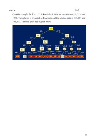
The document discusses backtracking as a general method for solving problems that involve systematically trying possibilities and abandoning partial solutions when they cannot possibly lead to a complete solution. It provides examples of applications of backtracking including the n-queens problem, sum of subsets problem, graph coloring, and finding Hamiltonian cycles in graphs. The general backtracking algorithm and terminology used are described. Specific algorithms for solving the n-queens problem and sum of subsets problem using backtracking are also presented.

![DAA
3
UNIT-4
Algorithm:
Algorithm Backtracking (n)
// Describes the backtracking procedure .All solutions are generated in X[1:n]
{
k=1;
While (k ≠ 0) do
{
if (there remains all untried
X[k] ϵ T (X[1],[2],…..X[k-1]) and Bk (X[1],…..X[k])) is true ) then
{
if(X[1],……X[k] )is the path to the answer node)
Then write(X[1:k]);
k=k+1; //consider the next step.
}
else k=k-1; //consider backtracking to the previous set.
}
}
All solutions are generated in X[1:n]
T(X[1]…..X[k-1]) is all possible values of X[k] gives that X[1],..........X[k-1]
have already been chosen.
Bk(X[1]………X[k]) is a bounding function which determines the elements of
X[k] which satisfies the implicit constraint.](https://image.slidesharecdn.com/daaunit-41-220616050646-9a215e9d/85/DAA-UNIT-4-1-pdf-3-320.jpg)


![DAA
13
UNIT-4
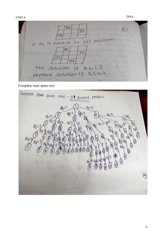
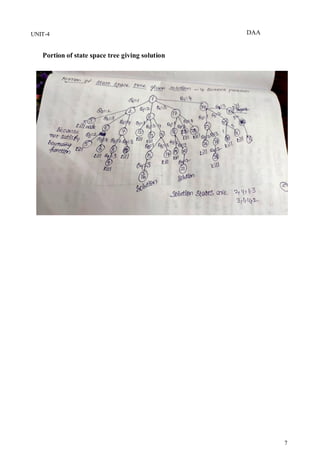
Built the state space tree
- Root represents an initial state
- Bodes reflect the specific choices made for the components of a solution
- Promising and non-promising nodes are present in the tree
Explore the state space tree using depth-first search
Prune non-promising nodes
- DFS stops exploring subtree rooted at nodes leading to no solution and
- backtracks to its parent node.
N-Queen Algorithm:
Algorithm N - Queens (k, n)
{
For i ← 1 to n
do if Place (k, i) then
{
x [k] ← i;
if (k ==n) then
write (x [1 ...n));
else
N - Queens (k + 1, n);
}
}
Place (k, i)
{
For j ← 1 to k - 1
do if (x [j] = i)
or (Abs x [j]) - i) = (Abs (j - k))
then return false;](https://image.slidesharecdn.com/daaunit-41-220616050646-9a215e9d/85/DAA-UNIT-4-1-pdf-13-320.jpg)

![DAA
20
UNIT-4
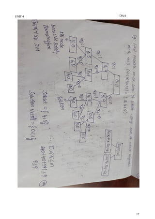
Sum of Subset Algorithm
Algorithm sumofsubset(s,k,r)
// find all subsets of w[1:n] that sum to m.
{
// Generate left child node. Note: s + w[k] ≤ m, since Bk-1 is true
x[k]=1;
if (s+w[k]=m) then write(x[1:k]); // Subset found
else if (s+w[k]+w[k+1] ≤ m)
then sumofsubset(s+w[k], k+1,r- w[k]);
// Generate right child and evaluate Bk
if ((s + r – w[k] ≥ m ) and (s + w[k+1] ≤ m)) then // exceeds m
{
x[k]=0;
sumofsubset(s, k+1, r-w[k]);
}}
Complexity
Time complexity = θ (2n
)
Space complexity = θ (1)](https://image.slidesharecdn.com/daaunit-41-220616050646-9a215e9d/85/DAA-UNIT-4-1-pdf-20-320.jpg)
![DAA
22
UNIT-4
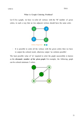
Working principle of graph coloring using backtracking
1. In backtracking approach, we color a single vertex and then move to its
adjacent (connected) vertex to color it with different color.
2. After coloring, we again move to another adjacent vertex that is uncolored
and repeat the process until all vertices of the given graph a re colored.
3. In case, we find a vertex that has all adjacent vertices colored and no color
is left to make it color different, we backtrack and change the color of the
last colored vertices and again proceed further.
4. By backtracking, we come back to the same vertex from where we started
and all colors were tried on it, then it means the given number of colors
(i.e. ‘m’) is insufficient to color the given graph and we require more
colors (i.e. a bigger chromatic number).
For many years it was known that five colors were sufficient to color any map, but
no map that required more than four colors had ever been found. After several hundred
years, this problem was solved by a group of mathematicians with the help of a
computer. They showed that in fact four colors are sufficient for planar graphs.
The function m-coloring will begin by first assigning the graph to its adjacency
matrix, setting the array x [] to zero. The colors are represented by the integers 1, 2, . .
. , m and the solutions are given by the n-tuple (x1, x2, . . ., xn), where xi is the color of
node i.](https://image.slidesharecdn.com/daaunit-41-220616050646-9a215e9d/85/DAA-UNIT-4-1-pdf-22-320.jpg)
![DAA
23
UNIT-4
A recursive backtracking algorithm for graph coloring is carried out by invoking the
statement mcoloring(1);
Algorithm mcoloring (k)
// This algorithm was formed using the recursive backtracking schema.
//The graph is represented by its Boolean adjacency matrix G [1: n, 1: n].
//All assignments of 1,2, ...m to the vertices of the graph such that adjacent vertices are
//assigned. k is the index of the next vertex to color.
{
repeat
{ // Generate all legal assignments for x[k].
NextValue (k); // Assign to x [k] a legal color.
If (x [k] = 0) then return; // No new color possible
If (k = n) then // at most m colors have been used to color the n vertices.
write (x [1: n]);
else mcoloring (k+1);
} until (false);
}
Algorithm NextValue (k)
// x[1],.......... x[k-1]have been assigned integer values in the range[1,m]such that
// adjacent vertices have distinct integers. A value for x [k] is determined in the range
// [0, m].x[k] is assigned the next highest numbered color while maintaining
distinctness
// from the adjacent vertices of vertex k. If no such color exists, then x [k] is 0.
{
repeat
{](https://image.slidesharecdn.com/daaunit-41-220616050646-9a215e9d/85/DAA-UNIT-4-1-pdf-23-320.jpg)
![DAA
24
UNIT-4
x [k]: = (x [k] +1) mod(m+1) // Next highest color.
If (x [k] = 0) then return; // All colors have been used
for j := 1 to n do
{ // check if this color is distinct from adjacent colors
if ((G [k, j] ≠ 0) and (x [k] = x[j]))
// If (k, j) is and edge and if adj. vertices have the same color.
then break;
}
if (j = n+1) then return; // New colorfound
}until(false); // Otherwise try to find anothercolor.
}
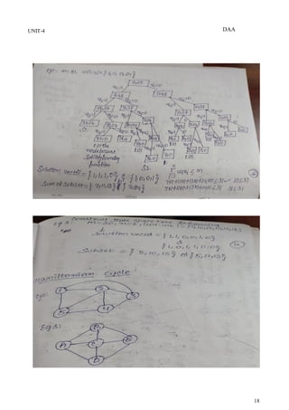
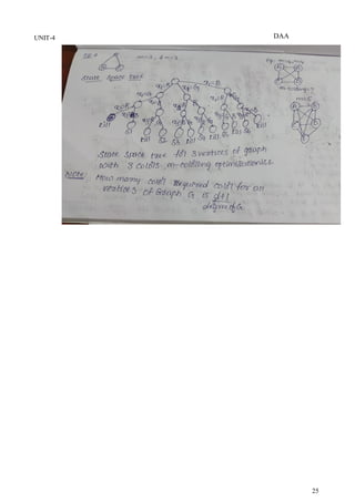
Example:
Color the graph given below with minimum number of colors by backtracking using
state space tree](https://image.slidesharecdn.com/daaunit-41-220616050646-9a215e9d/85/DAA-UNIT-4-1-pdf-24-320.jpg)

![DAA
33
UNIT-4
Again Backtrack
Here we have generated one Hamiltonian circuit, but another Hamiltonian circuit can
also be obtained by considering another vertex.
The backtracking solution vector (x1, . . . . . xn) is defined so that xi represents the ith
visited vertex of the proposed cycle. If k = 1, then x1 can be any of the n vertices. To
avoid printing the same cycle n times, we require that x1 = 1. If 1 < k < n, then xk can
be any vertex v that is distinct from x1,x2,...,xk–1 and v is connected by an edge to
kx-1. The vertex xn can only be one remaining vertex and it must be connected to both
xn-1 and x1.
Using NextValue algorithm we can particularize the recursive backtracking
schema to find all Hamiltonian cycles. This algorithm is started by first initializing the
adjacency matrix G[1: n, 1: n], then setting x[2: n] to zero and x[1] to 1, and then
executing Hamiltonian(2).
The traveling salesperson problem using dynamic programming asked for a tour that
has minimum cost. This tour is a Hamiltonian cycles. For the simple case of a graph all
of whose edge costs are identical, Hamiltonian will find a minimum-cost tour if a tour
exists.](https://image.slidesharecdn.com/daaunit-41-220616050646-9a215e9d/85/DAA-UNIT-4-1-pdf-33-320.jpg)
![DAA
34
UNIT-4
Algorithm NextValue (k)
// x [1: k-1] is a path of k – 1 distinct vertices . If x[k] = 0, then no vertex has as yet been
//assignedtox[k].Afterexecution,x[k]isassignedtothenexthighestnumberedvertex
//which does not already appear in x[1:k–1] and is connected by an edge to x[k–1].
// Otherwise x [k] = 0. If k = n, then in addition x [k] is connected to x [1].
{
repeat
x { [k] := (x [k] +1) mod(n+1); // Next vertex.
If(x[k] = 0) then return;
If (G [x [k – 1], x [k]] ≠ 0) then
{ // Is there an edge?
for j := 1 to k – 1 do
if (x [j] = x [k]) then break;
// check for distinctness.
If (j = k)then // If true, then the vertex is distinct.
If ((k < n) or ((k = n) and G [x [n], x [1]] ≠ 0))
then return;
}
} until (false);
}
Algorithm Hamiltonian (k)
// This algorithm uses the recursive formulation of backtracking to find all the
// Hamiltonian cycles of a graph. The graph is stored as an adjacency
// matrix G [1: n, 1: n]. All cycles begin at node 1.
{](https://image.slidesharecdn.com/daaunit-41-220616050646-9a215e9d/85/DAA-UNIT-4-1-pdf-34-320.jpg)
![DAA
35
UNIT-4
repeat
{
// Generate values for x[k].
NextValue (k); //Assign a legal Next value to x [k].
if (x [k] = 0) then return;
if (k = n) then
write (x [1: n]);
else
Hamiltonian (k + 1)
} until (false)](https://image.slidesharecdn.com/daaunit-41-220616050646-9a215e9d/85/DAA-UNIT-4-1-pdf-35-320.jpg)