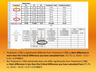
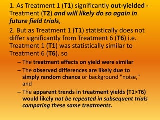
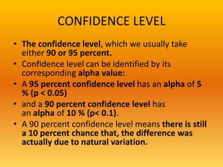
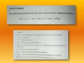
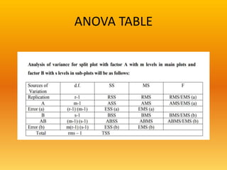
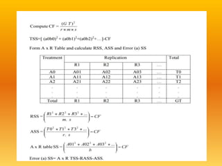
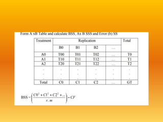
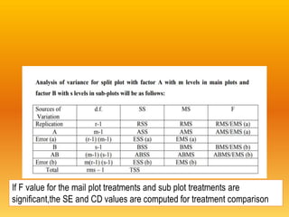
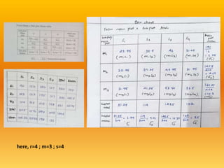
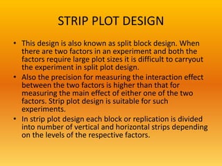
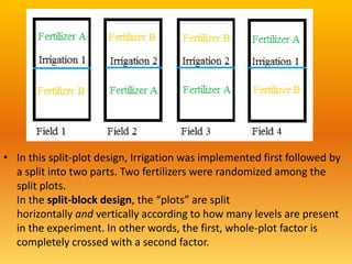
CriticalDifferencesinSplit plotand
Stripplot Design
K.ADITHYA
2022502301
TAMIL NADU AGRICULTURAL UNIVERSITY
STA 502 EXPERIMENTAL DESIGNS (2+1)
SPLIT PLOT DESIGN
• A split-plot design is an experimental design
in which researchers are interested in studying
two factors in which:
One of the factors is ā€œeasyā€ to change or vary.
One of the factors is ā€œhardā€ to change or vary.
• This type of design was developed in 1925 by
mathematician Ronald Fisher for use in
agricultural experiments.
• It occurs in factors which require larger plots than
for others.
• Eg: Experiments on Tillage and Irrigation require
larger plots whereas experiments on Fertilizers
and Herbicides require no larger plots.
• Larger plots are split into smaller plots to
accommodate the other factors; different
treatment where alloted at random to their
respective plots – Split plot design.
(Sub plots)
(Main plots)
CRITICAL DIFFERENCE
• Critical Difference is used to compare means
of different treatments that have an equal
number of replications.
• Treatment 1 (T1) is significantly different from Treatment 2 (T2) as their difference is
more than the Critical Difference you have calculated here. (T1-T2 i.e. 10.62 – 5.21 =
5.41 > 0.978887)
• But Treatment 1 (T1) statistically does not differ significantly from Treatment 6 (T6),
as their difference is less than the Critical Difference you have calculated here (T1-T6
i.e. 10.62 – 10.25 = 0.37 < 0.978887)
1. As Treatment 1 (T1) significantly out-yielded -
Treatment (T2) and will likely do so again in
future field trials,
2. But as Treatment 1 (T1) statistically does not
differ significantly from Treatment 6 (T6) i.e.
Treatment 1 (T1) was statistically similar to
Treatment 6 (T6). so
– The treatment effects on yield were similar
– The observed differences are likely due to
simply random chance or background "noise,"
and
– The apparent trends in treatment yields (T1>T6)
would likely not be repeated in subsequent trials
comparing these same treatments.
CONFIDENCE LEVEL
• The confidence level, which we usually take
either 90 or 95 percent.
• Confidence level can be identified by its
corresponding alpha value:
• A 95 percent confidence level has an alpha of 5
% (p < 0.05)
• and a 90 percent confidence level has
an alpha of 10 % (p< 0.1).
• A 90 percent confidence level means there is still
a 10 percent chance that, the difference was
actually due to natural variation.
ANOVA TABLE
here, r=4 ; m=3 ; s=4
STRIP PLOT DESIGN
• This design is also known as split block design. When
there are two factors in an experiment and both the
factors require large plot sizes it is difficult to carryout
the experiment in split plot design.
• Also the precision for measuring the interaction effect
between the two factors is higher than that for
measuring the main effect of either one of the two
factors. Strip plot design is suitable for such
experiments.
• In strip plot design each block or replication is divided
into number of vertical and horizontal strips depending
on the levels of the respective factors.
• In this split-plot design, Irrigation was implemented first followed by
a split into two parts. Two fertilizers were randomized among the
split plots.
In the split-block design, the ā€œplotsā€ are split
horizontally and vertically according to how many levels are present
in the experiment. In other words, the first, whole-plot factor is
completely crossed with a second factor.
Compute Correction Factor = (GT)²
-------------
a X b X r
TSS = Σyijk ²- CF
Trt SS = ΣYij²/r - CF
Blk SS= ΣY..k²/ ra - CF
1) Vertical Strip Analysis
Form A x R Table and calculate RSS, ASS and
Error(a) SS
2) Horizontal Strip Analysis
• Form B x R Table and calculate RSS, BSS and Error(b)
SS
3) Interaction Analysis
Form A xB Table and calculate BSS, Ax B SSS and Error
(b) SS
ANOVA
R=3
A=3
B=4
THANK YOU

critical differences in split plot and strip plot design.pptx

  • 1.
    CriticalDifferencesinSplit plotand Stripplot Design K.ADITHYA 2022502301 TAMILNADU AGRICULTURAL UNIVERSITY STA 502 EXPERIMENTAL DESIGNS (2+1)
  • 2.
    SPLIT PLOT DESIGN •A split-plot design is an experimental design in which researchers are interested in studying two factors in which: One of the factors is ā€œeasyā€ to change or vary. One of the factors is ā€œhardā€ to change or vary. • This type of design was developed in 1925 by mathematician Ronald Fisher for use in agricultural experiments.
  • 3.
    • It occursin factors which require larger plots than for others. • Eg: Experiments on Tillage and Irrigation require larger plots whereas experiments on Fertilizers and Herbicides require no larger plots. • Larger plots are split into smaller plots to accommodate the other factors; different treatment where alloted at random to their respective plots – Split plot design.
  • 4.
  • 5.
    CRITICAL DIFFERENCE • CriticalDifference is used to compare means of different treatments that have an equal number of replications.
  • 6.
    • Treatment 1(T1) is significantly different from Treatment 2 (T2) as their difference is more than the Critical Difference you have calculated here. (T1-T2 i.e. 10.62 – 5.21 = 5.41 > 0.978887) • But Treatment 1 (T1) statistically does not differ significantly from Treatment 6 (T6), as their difference is less than the Critical Difference you have calculated here (T1-T6 i.e. 10.62 – 10.25 = 0.37 < 0.978887)
  • 7.
    1. As Treatment1 (T1) significantly out-yielded - Treatment (T2) and will likely do so again in future field trials, 2. But as Treatment 1 (T1) statistically does not differ significantly from Treatment 6 (T6) i.e. Treatment 1 (T1) was statistically similar to Treatment 6 (T6). so – The treatment effects on yield were similar – The observed differences are likely due to simply random chance or background "noise," and – The apparent trends in treatment yields (T1>T6) would likely not be repeated in subsequent trials comparing these same treatments.
  • 8.
    CONFIDENCE LEVEL • Theconfidence level, which we usually take either 90 or 95 percent. • Confidence level can be identified by its corresponding alpha value: • A 95 percent confidence level has an alpha of 5 % (p < 0.05) • and a 90 percent confidence level has an alpha of 10 % (p< 0.1). • A 90 percent confidence level means there is still a 10 percent chance that, the difference was actually due to natural variation.
  • 10.
  • 24.
    here, r=4 ;m=3 ; s=4
  • 28.
    STRIP PLOT DESIGN •This design is also known as split block design. When there are two factors in an experiment and both the factors require large plot sizes it is difficult to carryout the experiment in split plot design. • Also the precision for measuring the interaction effect between the two factors is higher than that for measuring the main effect of either one of the two factors. Strip plot design is suitable for such experiments. • In strip plot design each block or replication is divided into number of vertical and horizontal strips depending on the levels of the respective factors.
  • 29.
    • In thissplit-plot design, Irrigation was implemented first followed by a split into two parts. Two fertilizers were randomized among the split plots. In the split-block design, the ā€œplotsā€ are split horizontally and vertically according to how many levels are present in the experiment. In other words, the first, whole-plot factor is completely crossed with a second factor.
  • 30.
    Compute Correction Factor= (GT)² ------------- a X b X r TSS = Σyijk ²- CF Trt SS = ΣYij²/r - CF Blk SS= ΣY..k²/ ra - CF
  • 31.
    1) Vertical StripAnalysis Form A x R Table and calculate RSS, ASS and Error(a) SS
  • 33.
    2) Horizontal StripAnalysis • Form B x R Table and calculate RSS, BSS and Error(b) SS
  • 35.
    3) Interaction Analysis FormA xB Table and calculate BSS, Ax B SSS and Error (b) SS
  • 36.
  • 44.
  • 48.