This PPT provides basic knowledge for those interested in analyzing experimental data.

1. Basic statistical
analysis of
experimental data

2. 1. Basics of experimental design
1.1. Complete blocks
1.2. Incomplete blocks
2. Basic principles of data analysis
2.1. Univariate analysis of single factor experiments
2.2. Univariate analysis of factorial experiments
2.2.1. Normal responses – ANOVA & LMM
2.2.2. Non-normal responses – GLMS, GLMM, NLMM
2.3. Univariate analysis of multi-site multi-year data
2.4. Multivariate analysis (MANOVA)
3. Communicating uncertainty
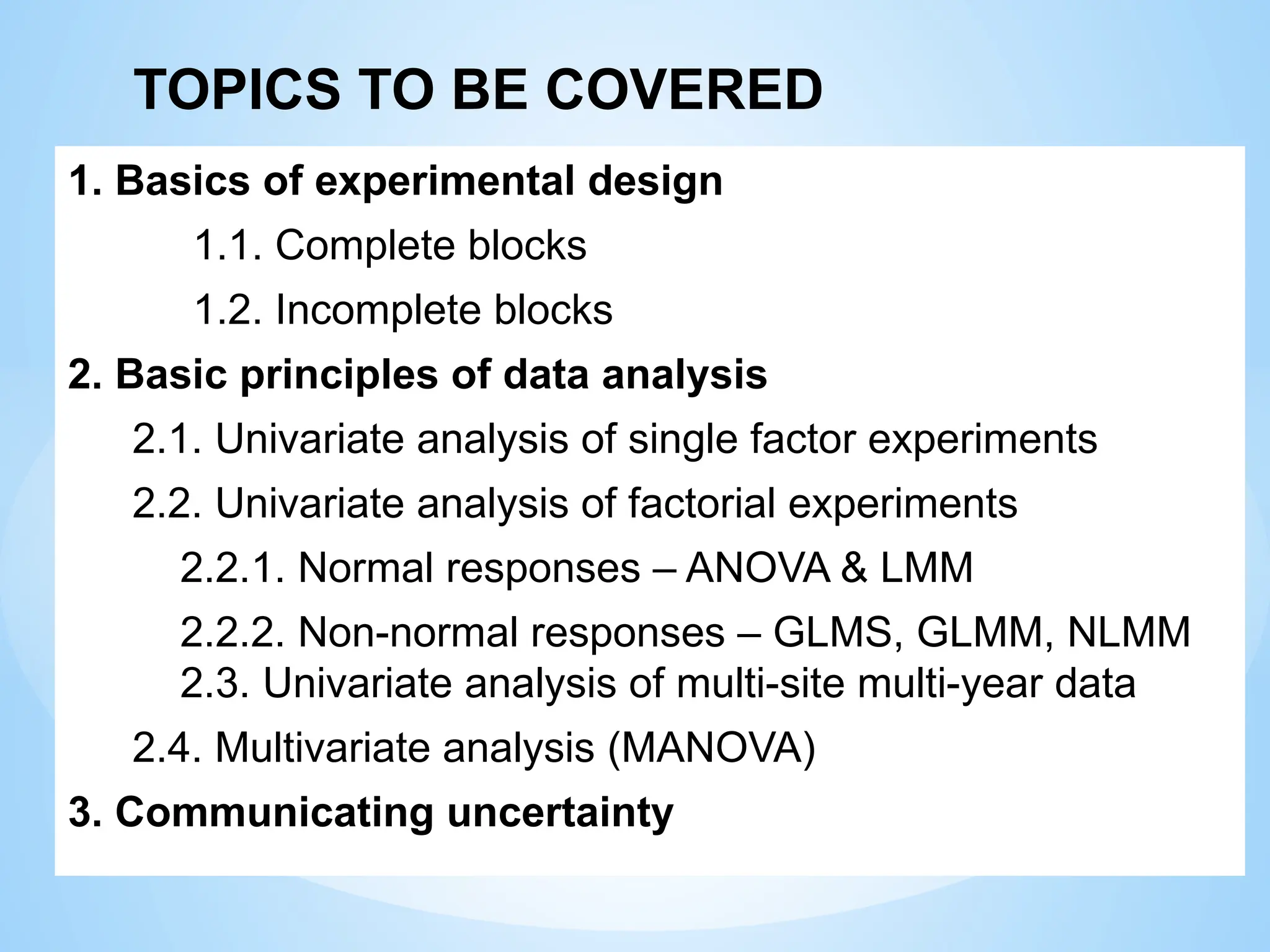
TOPICS TO BE COVERED

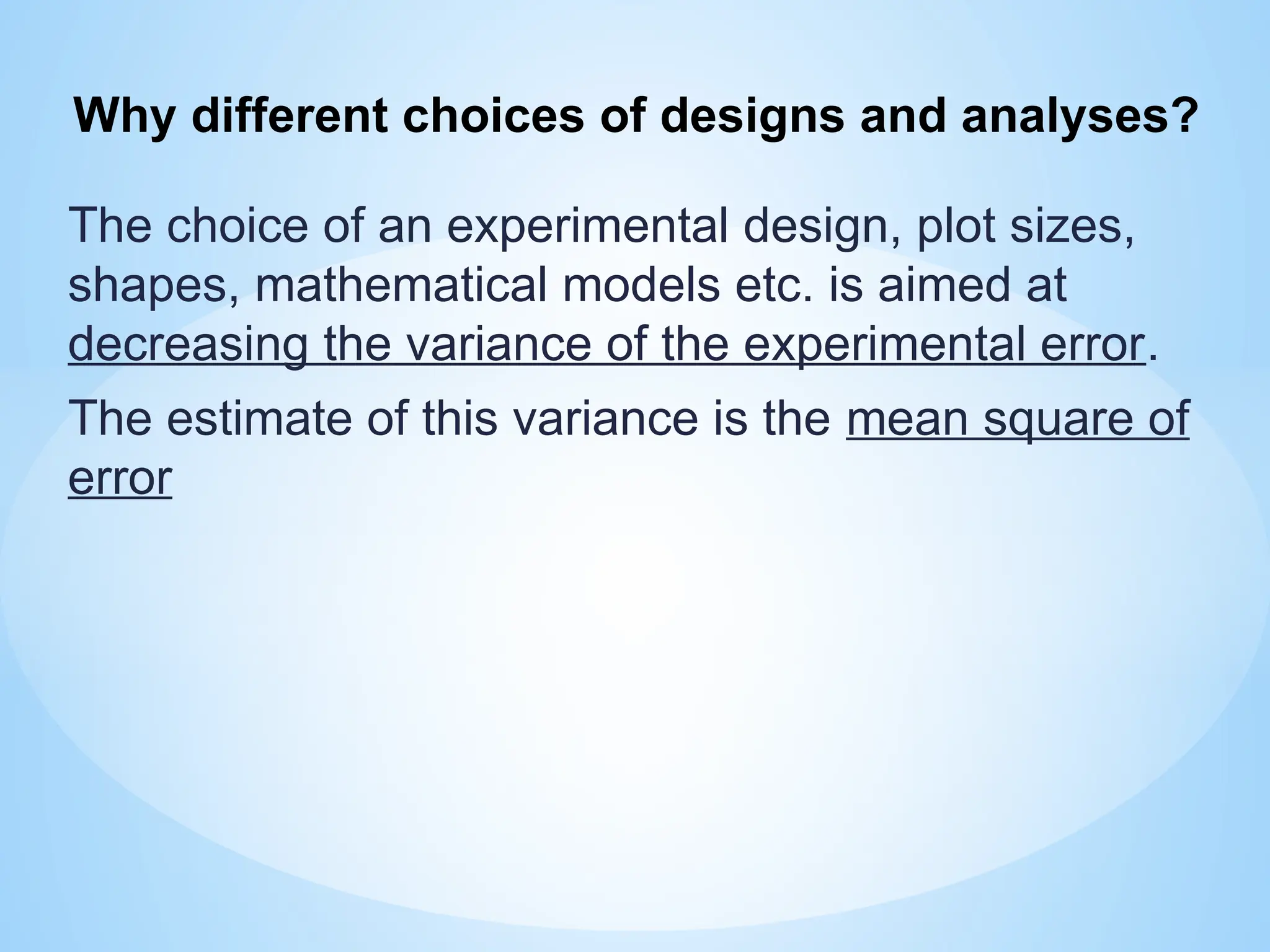
3. The choice of an experimental design, plot sizes,
shapes, mathematical models etc. is aimed at
decreasing the variance of the experimental error.
The estimate of this variance is the mean square of
error
Why different choices of designs and analyses?

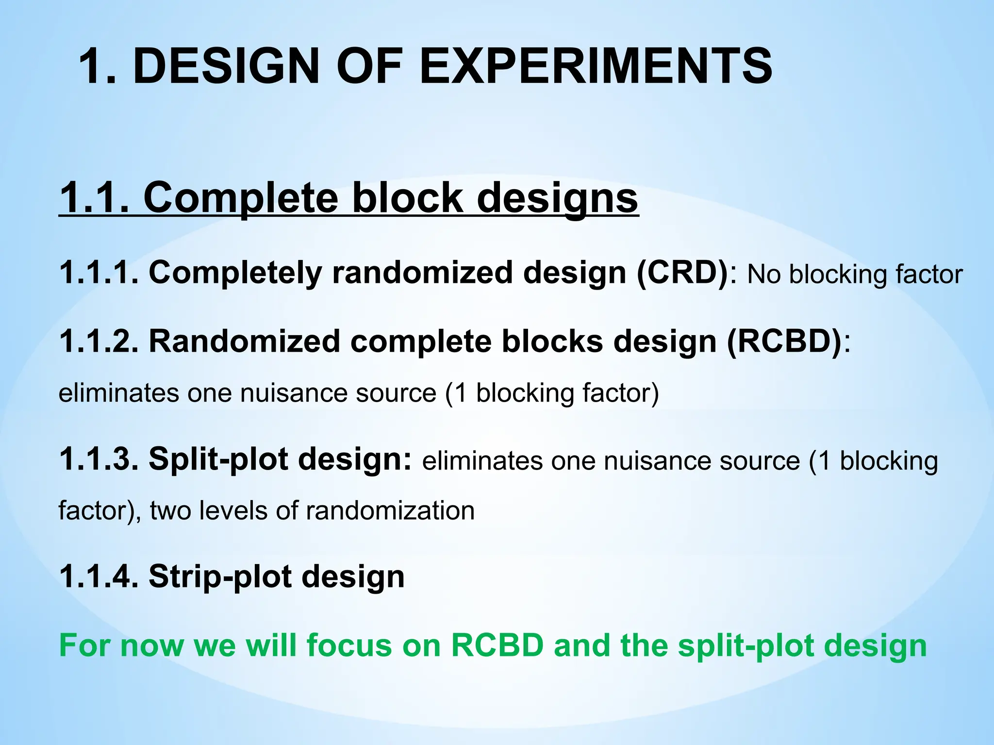
4. 1. DESIGN OF EXPERIMENTS
1.1. Complete block designs
1.1.1. Completely randomized design (CRD): No blocking factor
1.1.2. Randomized complete blocks design (RCBD):
eliminates one nuisance source (1 blocking factor)
1.1.3. Split-plot design: eliminates one nuisance source (1 blocking
factor), two levels of randomization
1.1.4. Strip-plot design
For now we will focus on RCBD and the split-plot design

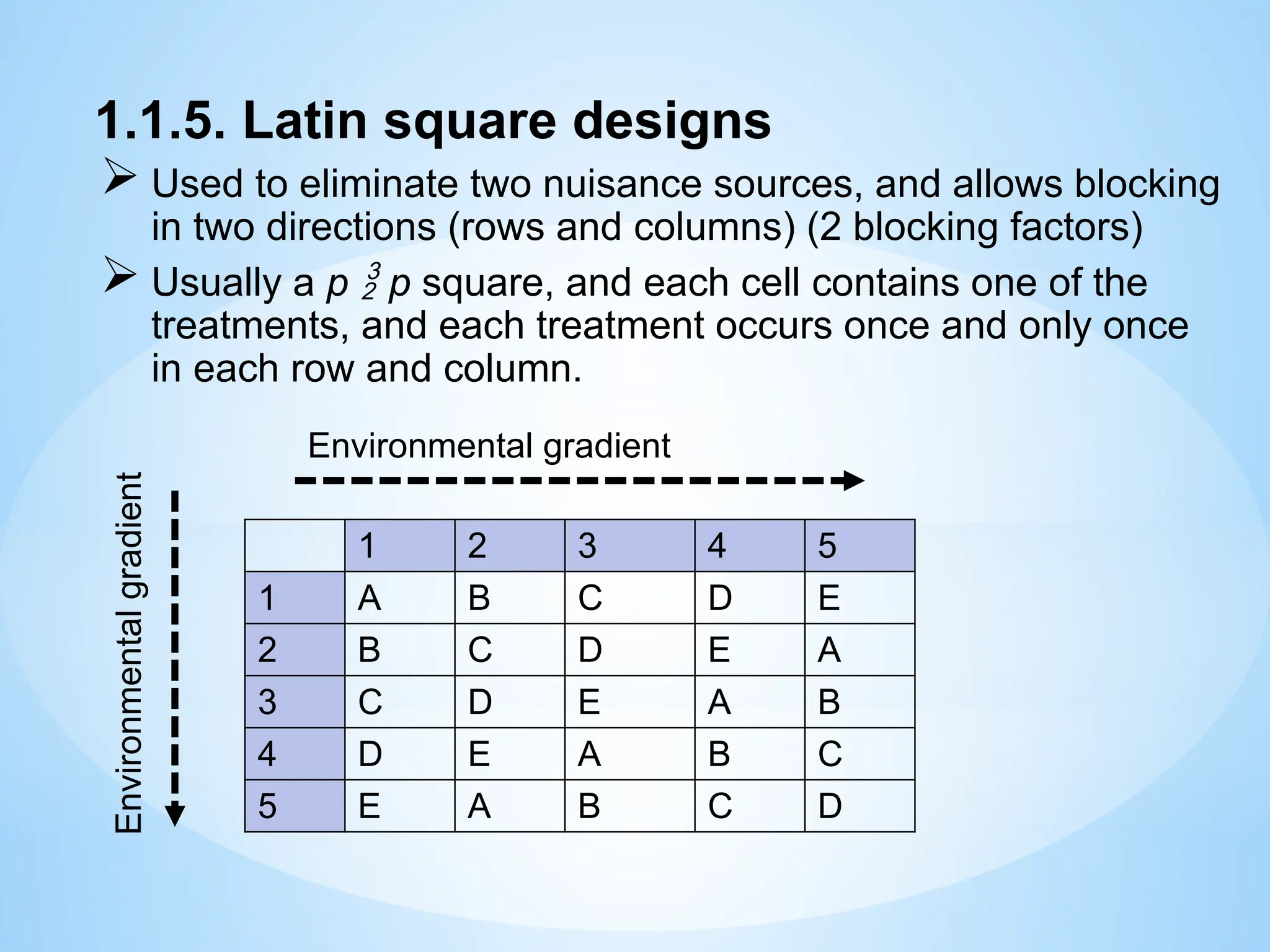
5. 1.1.5. Latin square designs
 Used to eliminate two nuisance sources, and allows blocking
in two directions (rows and columns) (2 blocking factors)
 Usually a p  p square, and each cell contains one of the
treatments, and each treatment occurs once and only once
in each row and column.
1 2 3 4 5
1 A B C D E
2 B C D E A
3 C D E A B
4 D E A B C
5 E A B C D
Environmental gradient
Environmental
gradient

6. 1.2. Incomplete blocks designs
When the number of treatments is large (T>20), e.g. variety
trials, complete block designs become unsuitable because
as the size of the block increases soil heterogeneity
increases.
This increases the experimental error and diminishes the
researcher's ability to observe significance differences
between any two treatments.
In such cases incomplete block designs are more efficient
Every block only contains a fraction of the total number of
treatments and is therefore incomplete. Several incomplete
blocks form one complete replication.
E.g. Lattice design

7. 1.2.1. Lattice designs
Types of lattice design
1.2.1.1. Square Lattices: a quadratic or cubic number of
treatments (e.g. 9, 16, 25, etc). The number of plots per block
(k) has to be the square root of the number of treatments (T),
e.g. 36 treatments in 6 blocks of 6 plots per replicate.
1.2.1.2. Rectangular Lattices: The number of treatments has
to equal k(k+1) with k= number of treatments per block. This
algorithm allows for treatment numbers like 12 or 20.
1.2.1.3. Alpha-designs (generalised lattices): Conditions
The number of plots per block (k) has to be ≤√T
The number of replicates has to be ≤T/k
The number of treatments has to be a multiple of k.

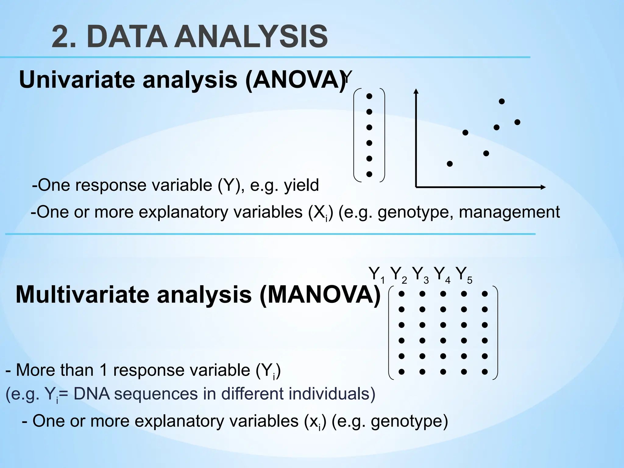
8. -One response variable (Y), e.g. yield
-One or more explanatory variables (Xi) (e.g. genotype, management
- More than 1 response variable (Yi)
(e.g. Yi= DNA sequences in different individuals)
- One or more explanatory variables (xi) (e.g. genotype)
Y
Y1 Y2 Y3 Y4 Y5
Univariate analysis (ANOVA)
Multivariate analysis (MANOVA)
2. DATA ANALYSIS

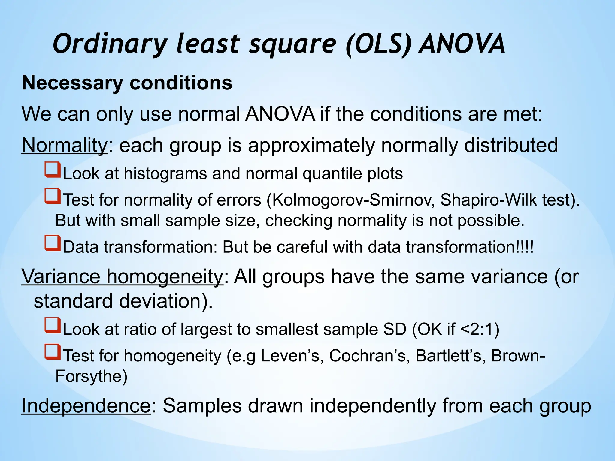
9. Ordinary least square (OLS) ANOVA
Necessary conditions
We can only use normal ANOVA if the conditions are met:
Normality: each group is approximately normally distributed
Look at histograms and normal quantile plots
Test for normality of errors (Kolmogorov-Smirnov, Shapiro-Wilk test).
But with small sample size, checking normality is not possible.
Data transformation: But be careful with data transformation!!!!
Variance homogeneity: All groups have the same variance (or
standard deviation).
Look at ratio of largest to smallest sample SD (OK if <2:1)
Test for homogeneity (e.g Leven’s, Cochran’s, Bartlett’s, Brown-
Forsythe)
Independence: Samples drawn independently from each group

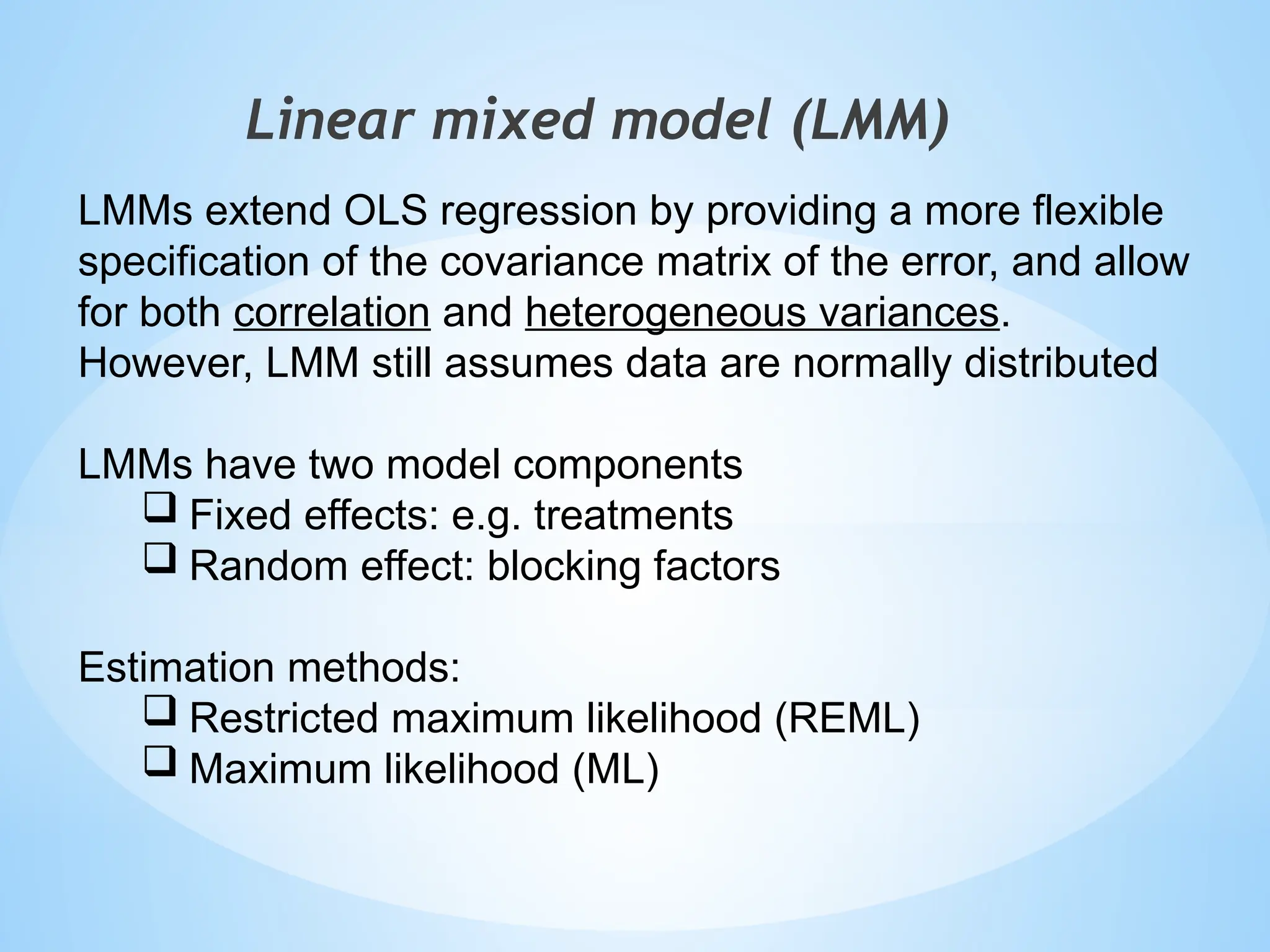
10. Linear mixed model (LMM)
LMMs extend OLS regression by providing a more flexible
specification of the covariance matrix of the error, and allow
for both correlation and heterogeneous variances.
However, LMM still assumes data are normally distributed
LMMs have two model components
 Fixed effects: e.g. treatments
 Random effect: blocking factors
Estimation methods:
 Restricted maximum likelihood (REML)
 Maximum likelihood (ML)

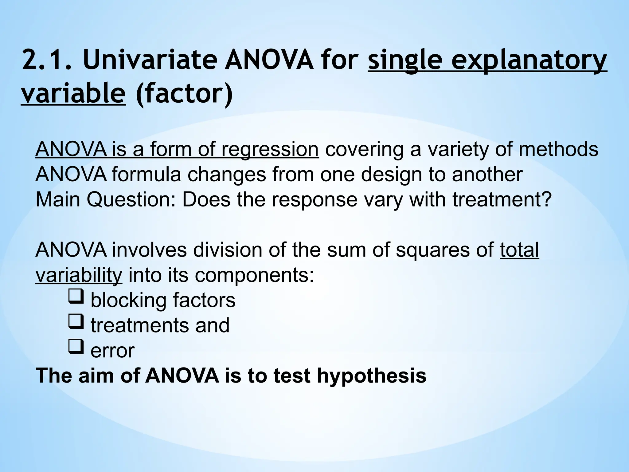
11. 2.1. Univariate ANOVA for single explanatory
variable (factor)
ANOVA is a form of regression covering a variety of methods
ANOVA formula changes from one design to another
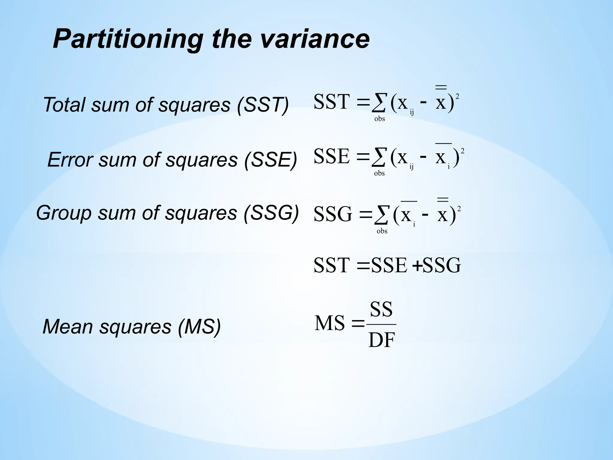
Main Question: Does the response vary with treatment?
ANOVA involves division of the sum of squares of total
variability into its components:
 blocking factors
 treatments and
 error
The aim of ANOVA is to test hypothesis

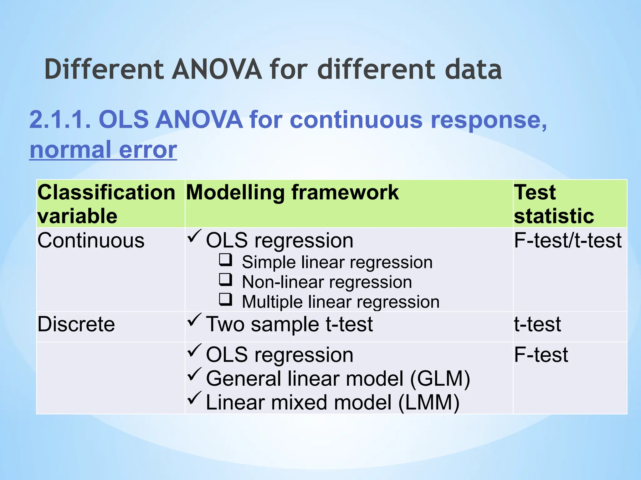
12. Classification
variable
Modelling framework Test
statistic
Continuous OLS regression
 Simple linear regression
 Non-linear regression
 Multiple linear regression
F-test/t-test
Discrete Two sample t-test t-test
OLS regression
General linear model (GLM)
Linear mixed model (LMM)
F-test
Different ANOVA for different data
2.1.1. OLS ANOVA for continuous response,
normal error

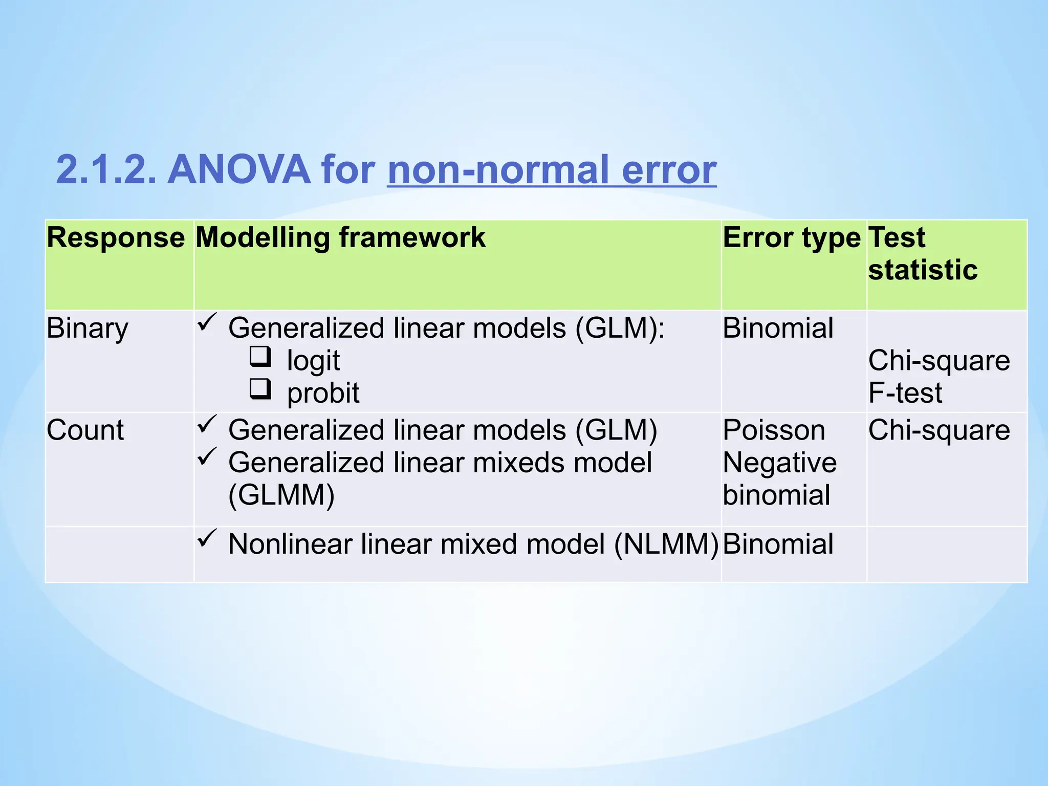
13. Response Modelling framework Error type Test
statistic
Binary  Generalized linear models (GLM):
 logit
 probit
Binomial
Chi-square
F-test
Count  Generalized linear models (GLM)
 Generalized linear mixeds model
(GLMM)
Poisson
Negative
binomial
Chi-square
 Nonlinear linear mixed model (NLMM)Binomial
2.1.2. ANOVA for non-normal error

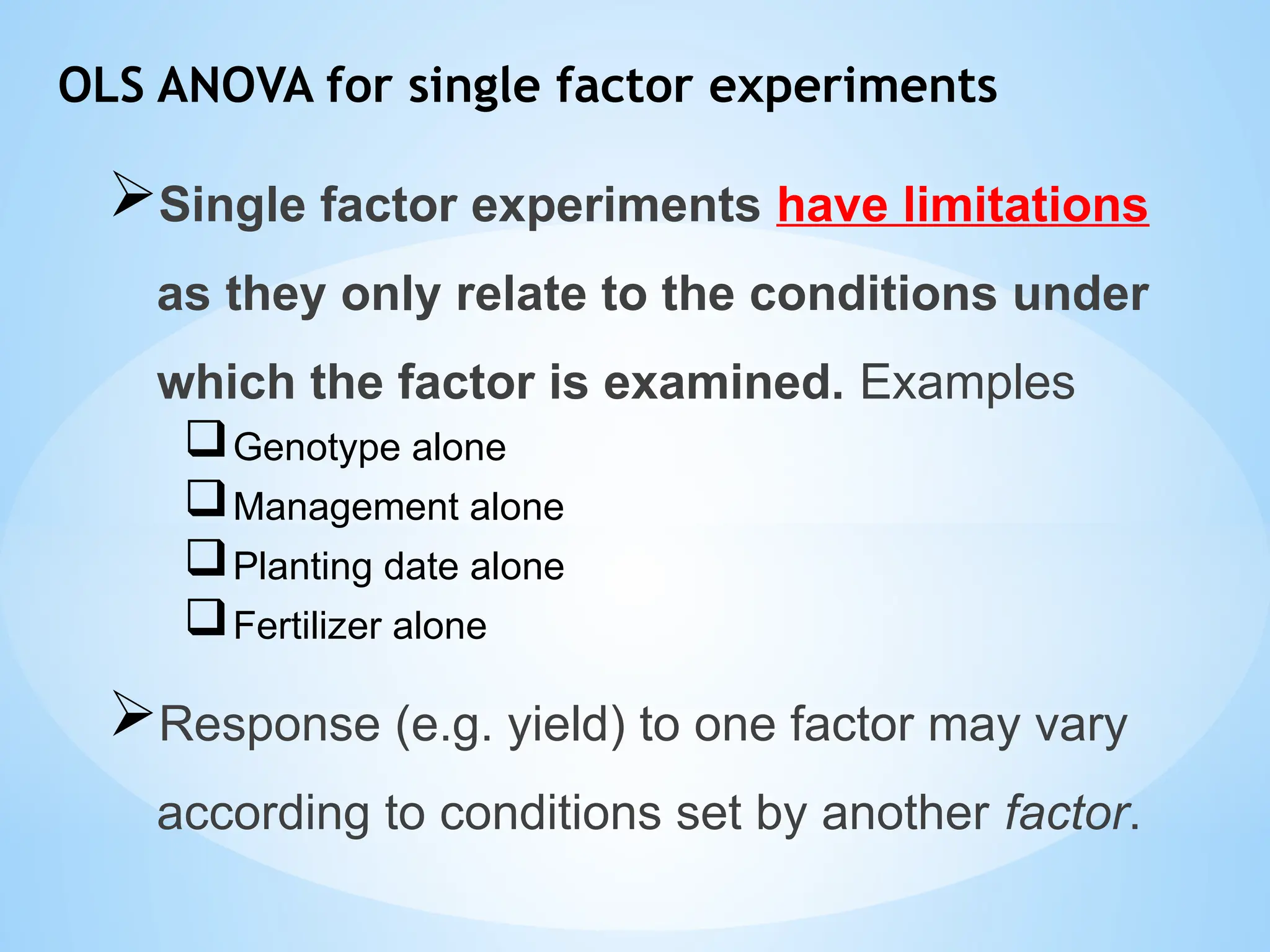
14. OLS ANOVA for single factor experiments
Single factor experiments have limitations
as they only relate to the conditions under
which the factor is examined. Examples
Genotype alone
Management alone
Planting date alone
Fertilizer alone
Response (e.g. yield) to one factor may vary
according to conditions set by another factor.

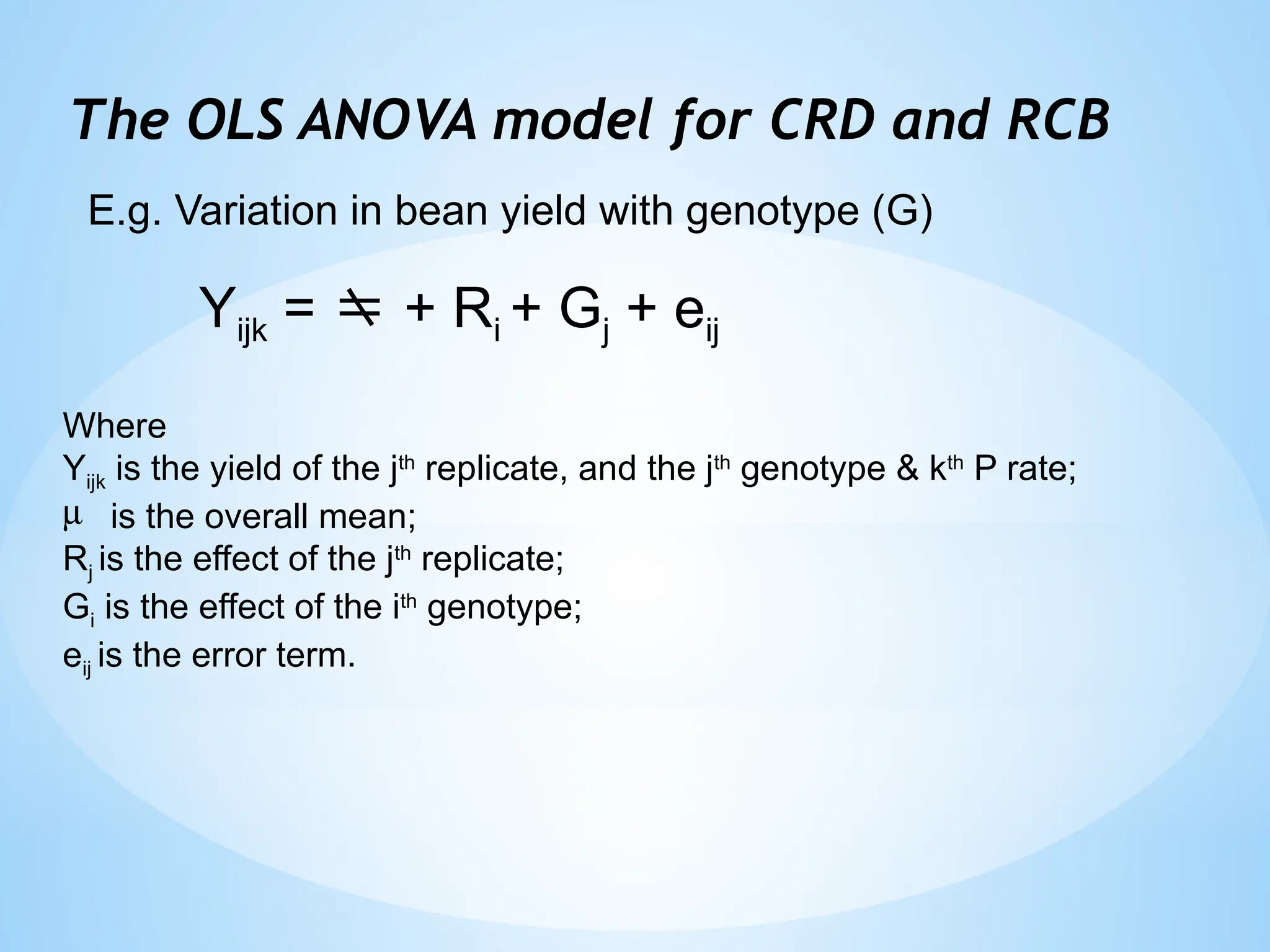
15. The OLS ANOVA model for CRD and RCB
Yijk =  + Ri + Gj + eij
Where
Yijk is the yield of the jth
replicate, and the jth
genotype & kth
P rate;
m is the overall mean;
Rj is the effect of the jth
replicate;
Gi is the effect of the ith
genotype;
eij is the error term.
E.g. Variation in bean yield with genotype (G)

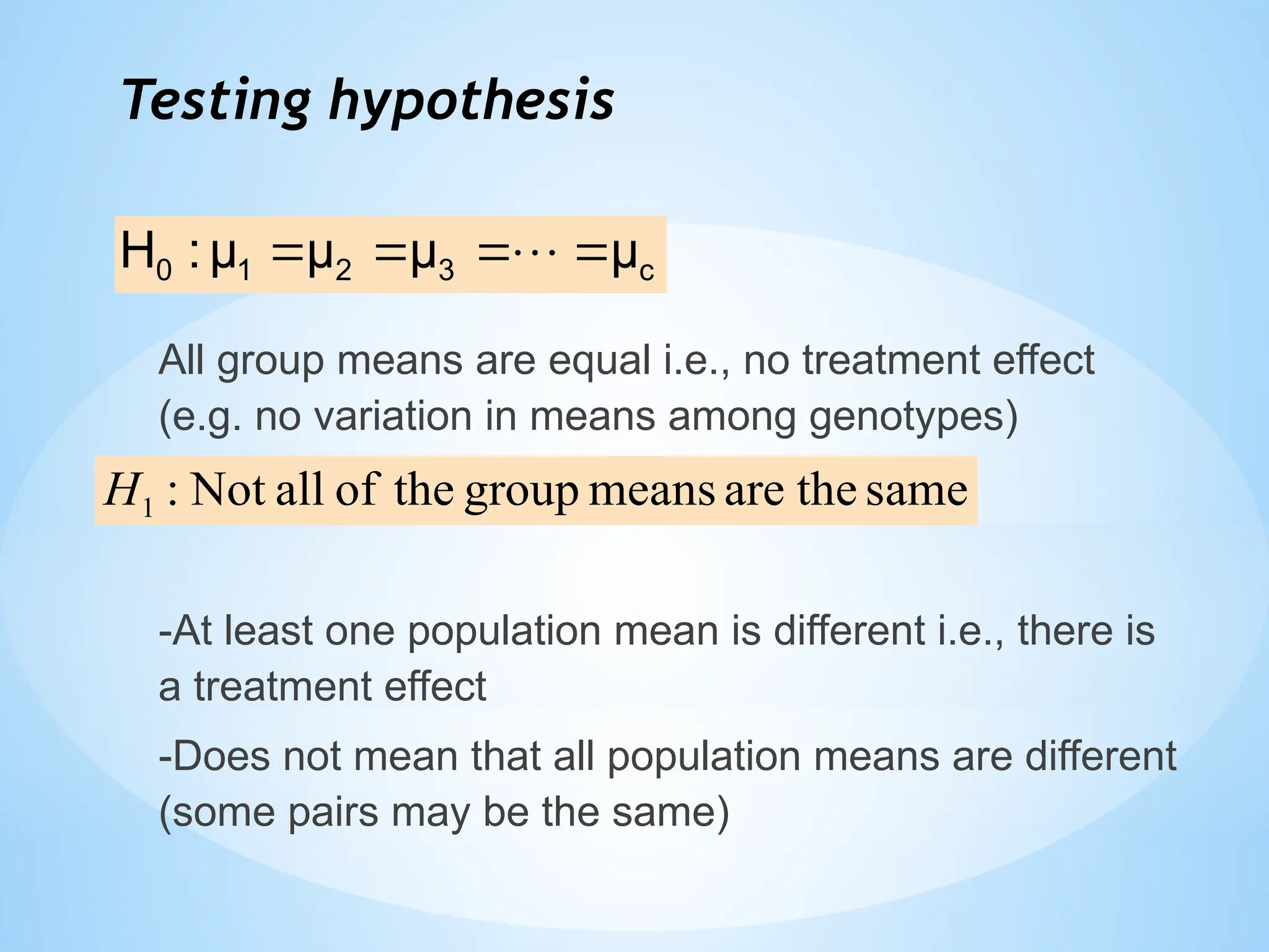
16. Testing hypothesis
All group means are equal i.e., no treatment effect
(e.g. no variation in means among genotypes)
-At least one population mean is different i.e., there is
a treatment effect
-Does not mean that all population means are different
(some pairs may be the same)
c
3
2
1
0 μ
μ
μ
μ
:
H 


 
same
the
are
means
group
the
of
all
Not
:
1
H

17. Partitioning the variance
DF
SS
MS
SSG
SSE
SST
)
x
x
(
SSG
)
x
(x
SSE
)
x
(x
SST
2
obs
i
obs
2
i
ij
2
obs
ij












Total sum of squares (SST)
Error sum of squares (SSE)
Group sum of squares (SSG)
Mean squares (MS)

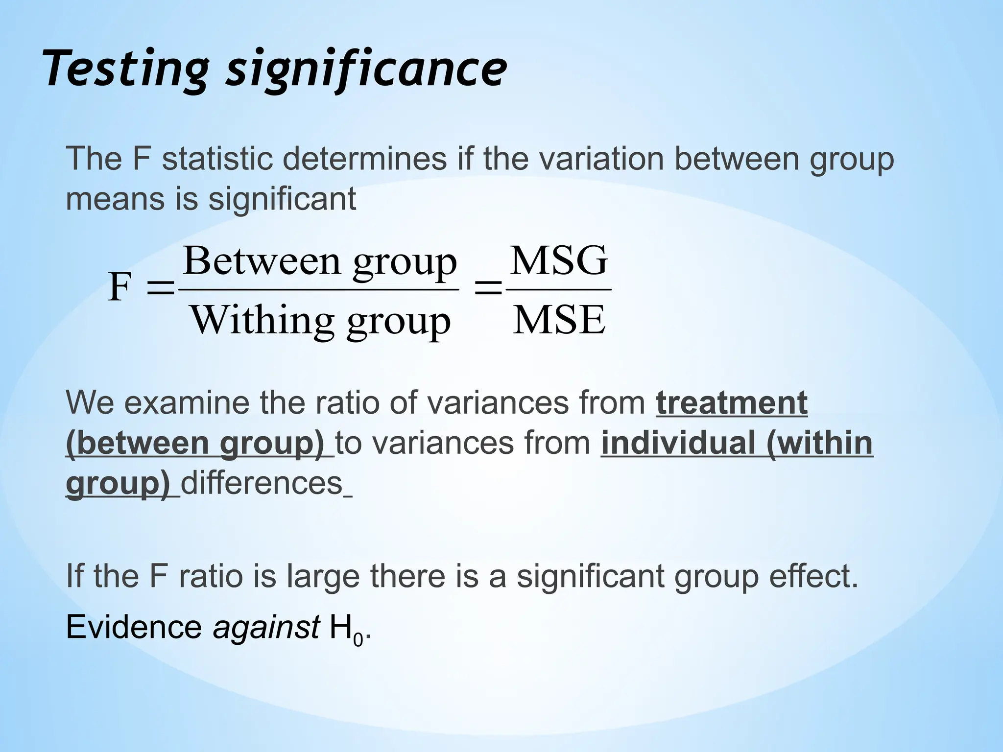
18. Testing significance
The F statistic determines if the variation between group
means is significant
We examine the ratio of variances from treatment
(between group) to variances from individual (within
group) differences
If the F ratio is large there is a significant group effect.
Evidence against H0.
MSE
MSG
group
Withing
group
Between
F 


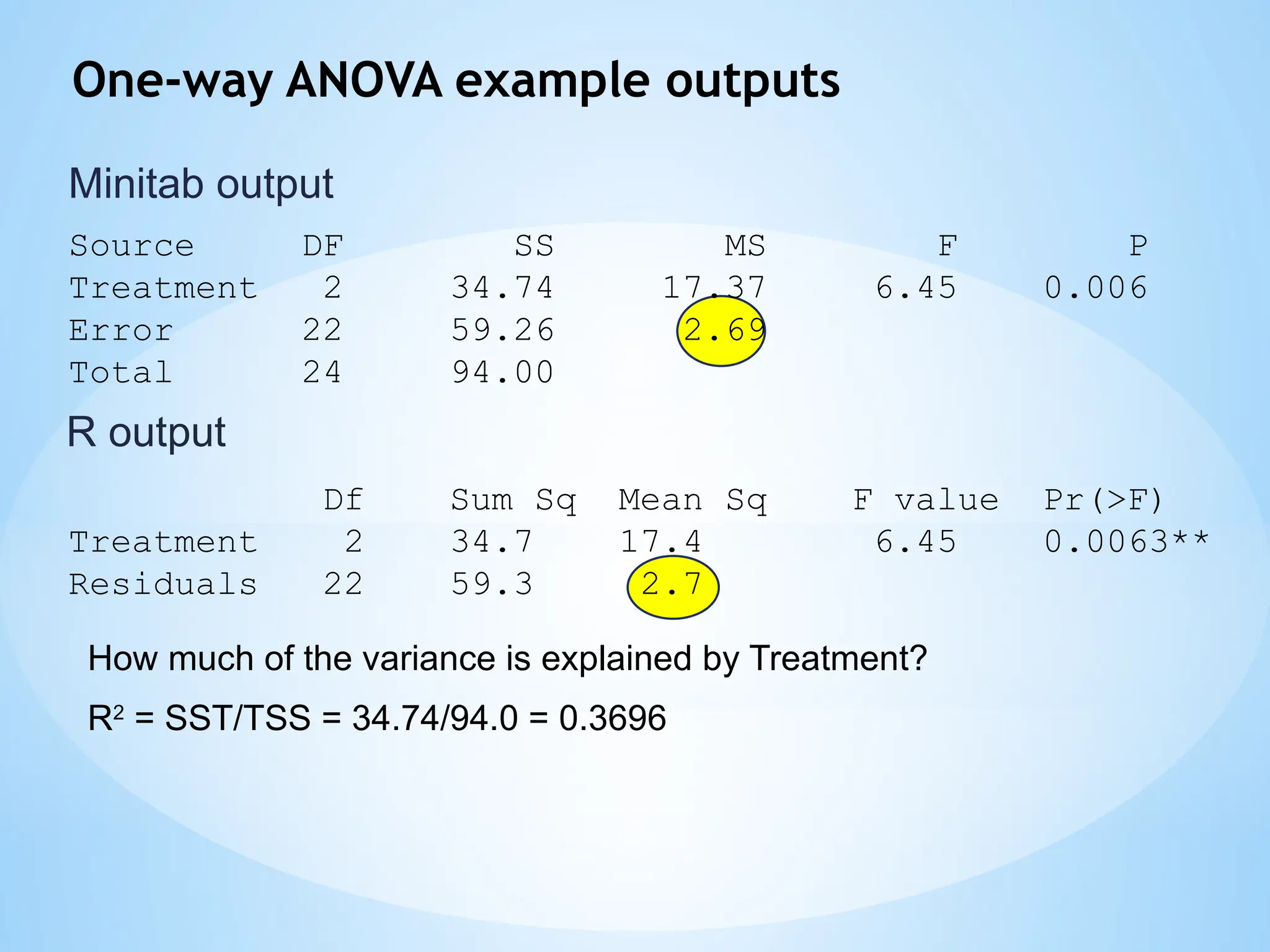
19. One-way ANOVA example outputs
Source DF SS MS F P
Treatment 2 34.74 17.37 6.45 0.006
Error 22 59.26 2.69
Total 24 94.00
Df Sum Sq Mean Sq F value Pr(>F)
Treatment 2 34.7 17.4 6.45 0.0063**
Residuals 22 59.3 2.7
R output
Minitab output
How much of the variance is explained by Treatment?
R2
= SST/TSS = 34.74/94.0 = 0.3696

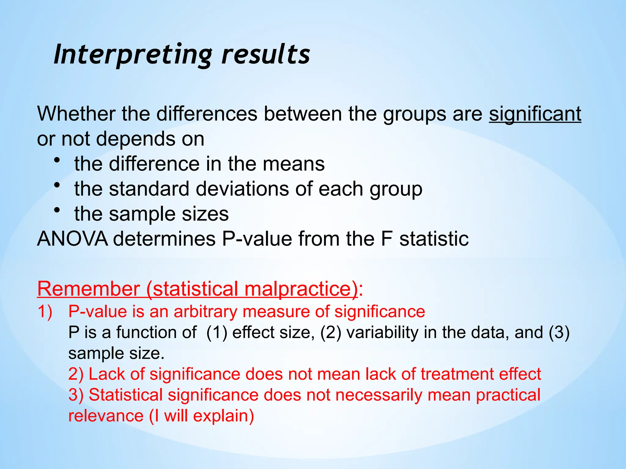
20. Interpreting results
Whether the differences between the groups are significant
or not depends on
• the difference in the means
• the standard deviations of each group
• the sample sizes
ANOVA determines P-value from the F statistic
Remember (statistical malpractice):
1) P-value is an arbitrary measure of significance
P is a function of (1) effect size, (2) variability in the data, and (3)
sample size.
2) Lack of significance does not mean lack of treatment effect
3) Statistical significance does not necessarily mean practical
relevance (I will explain)

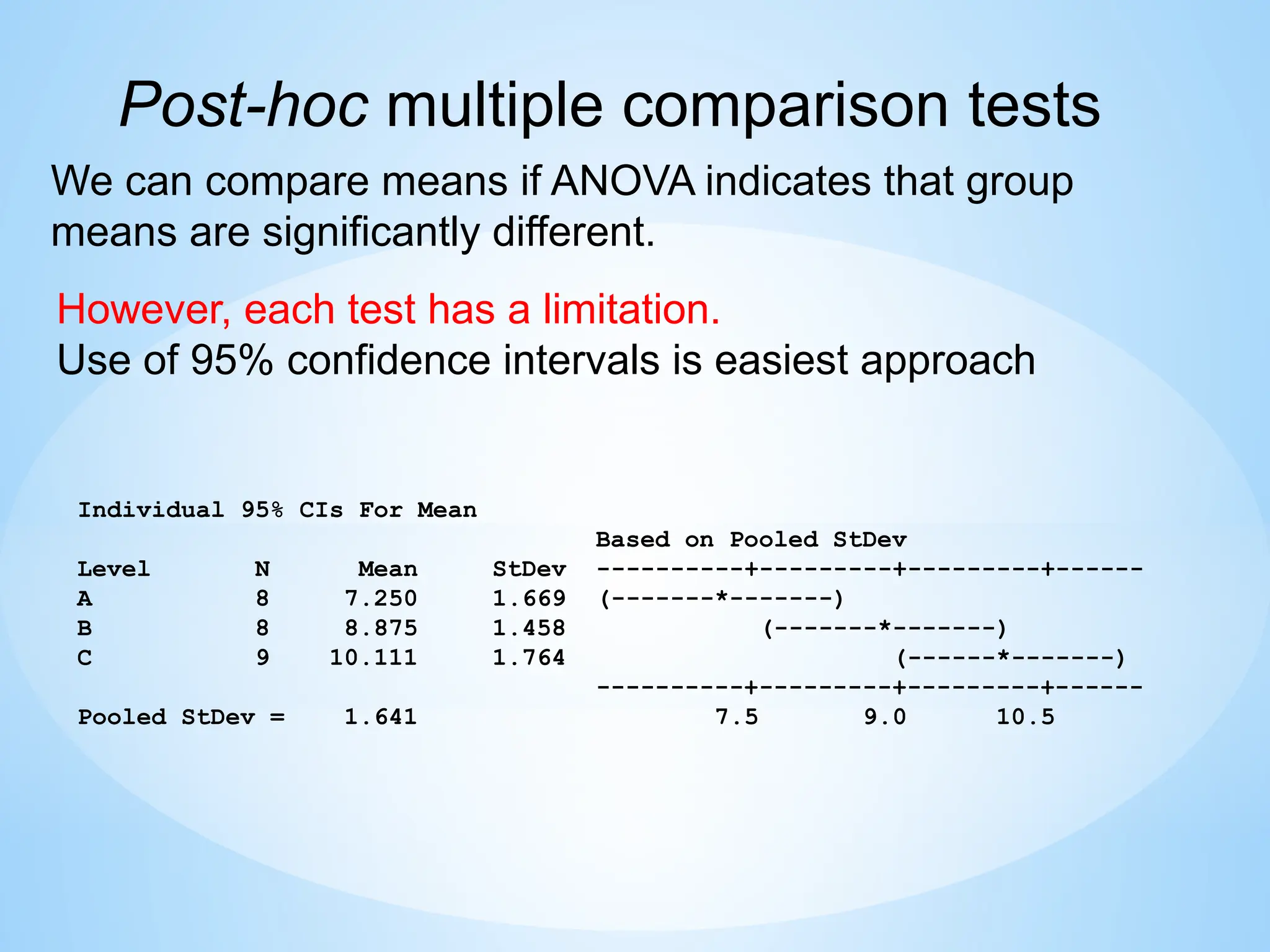
21. Individual 95% CIs For Mean
Based on Pooled StDev
Level N Mean StDev ----------+---------+---------+------
A 8 7.250 1.669 (-------*-------)
B 8 8.875 1.458 (-------*-------)
C 9 10.111 1.764 (------*-------)
----------+---------+---------+------
Pooled StDev = 1.641 7.5 9.0 10.5
We can compare means if ANOVA indicates that group
means are significantly different.
However, each test has a limitation.
Use of 95% confidence intervals is easiest approach
Post-hoc multiple comparison tests

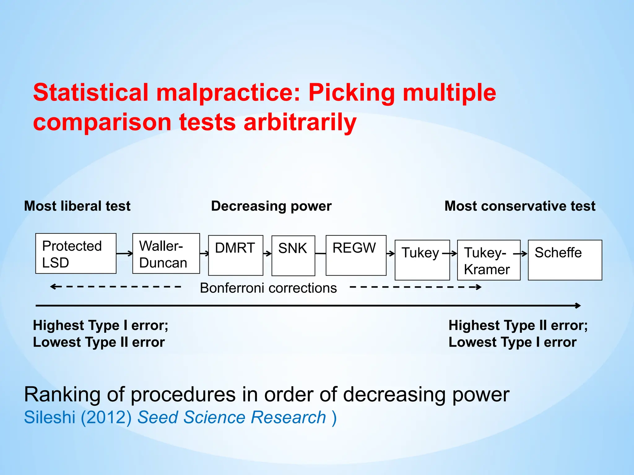
22. Decreasing power
Protected
LSD
SNK
DMRT Tukey-
Kramer
Scheffe
Tukey
Highest Type I error;
Lowest Type II error
Highest Type II error;
Lowest Type I error
Bonferroni corrections
Most liberal test Most conservative test
REGW
Waller-
Duncan
Ranking of procedures in order of decreasing power
Sileshi (2012) Seed Science Research )
Statistical malpractice: Picking multiple
comparison tests arbitrarily

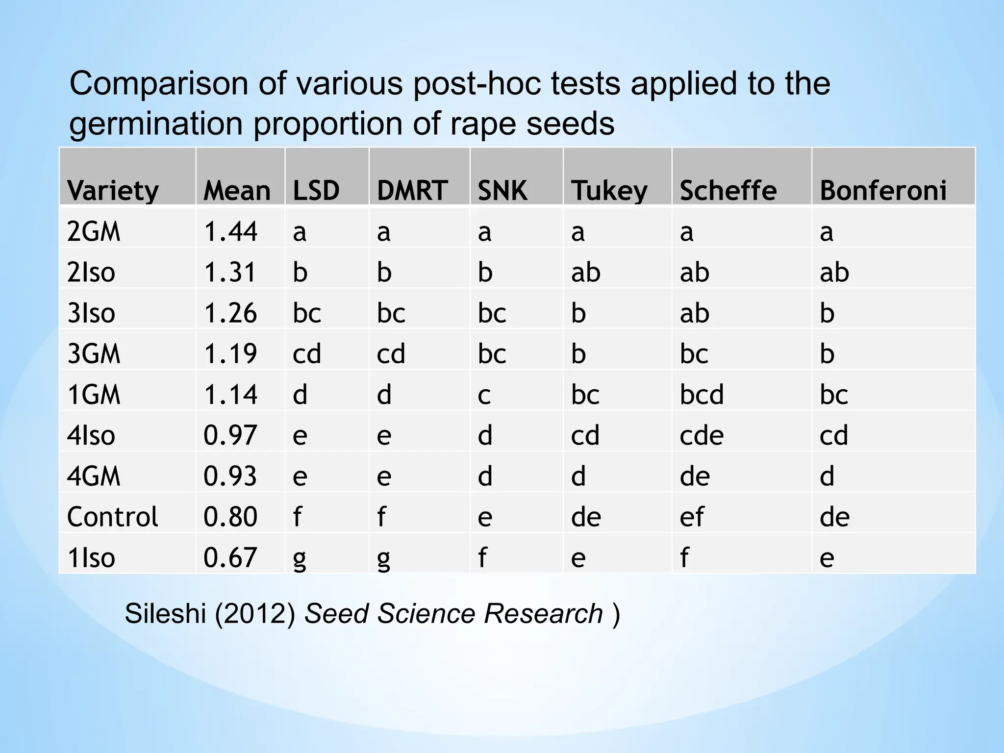
23. Variety Mean LSD DMRT SNK Tukey Scheffe Bonferoni
2GM 1.44 a a a a a a
2Iso 1.31 b b b ab ab ab
3Iso 1.26 bc bc bc b ab b
3GM 1.19 cd cd bc b bc b
1GM 1.14 d d c bc bcd bc
4Iso 0.97 e e d cd cde cd
4GM 0.93 e e d d de d
Control 0.80 f f e de ef de
1Iso 0.67 g g f e f e
Comparison of various post-hoc tests applied to the
germination proportion of rape seeds
Sileshi (2012) Seed Science Research )

24. ANOVA for more than one independent factors: A
design where all possible combinations of two (or more)
factors is called a factorial design
Control for confounders
Test for interactions between predictors
Improve predictions
2.2. Analysis of factorial experiments in detail
 Factorial designs are usually balanced. Unbalanced
designs are possible but not advised.
 Examine the effect of differences between factor A levels.
 Examine the effect of differences between factor B levels.
 Examine the interaction between levels of factor A and B

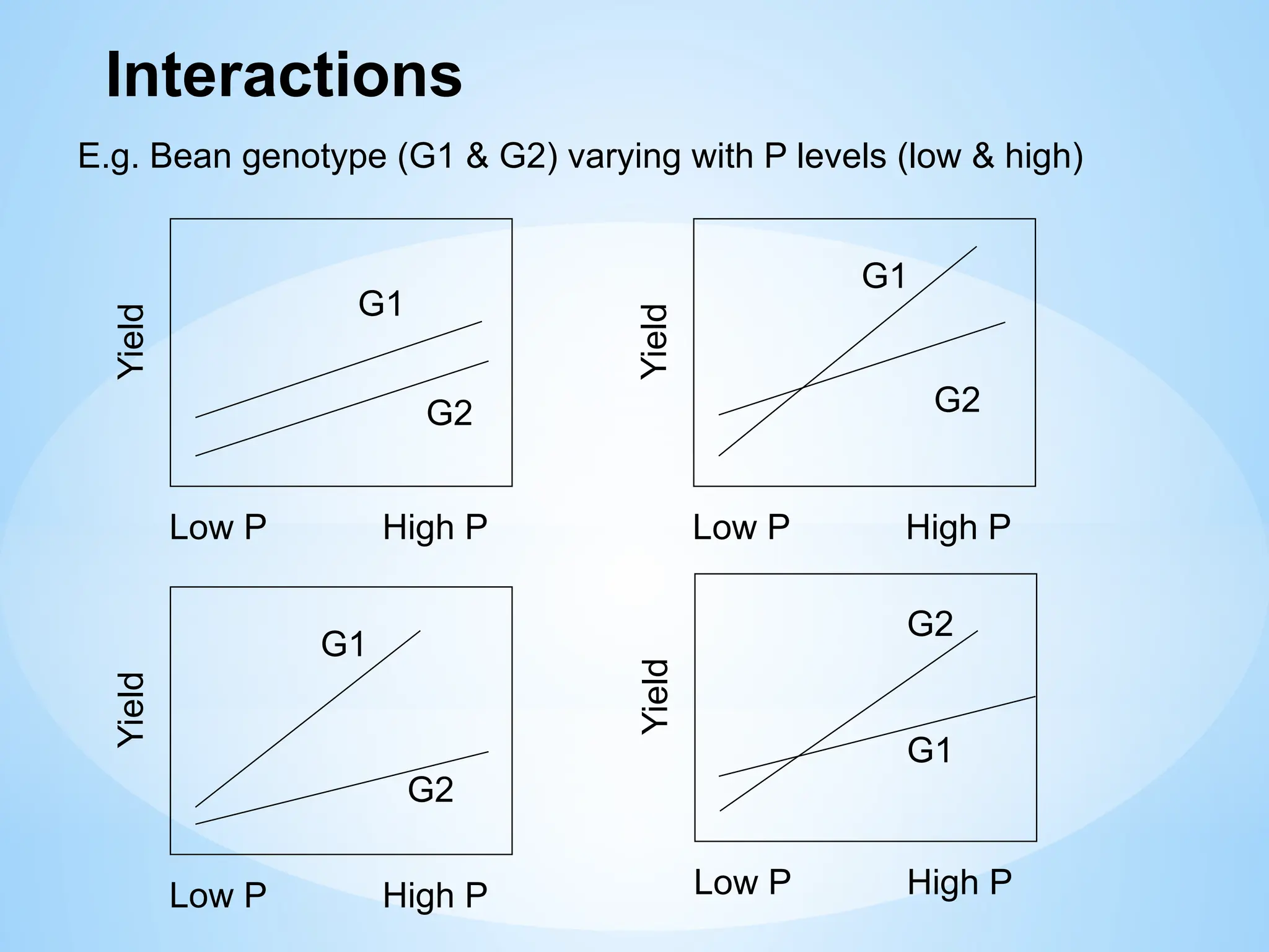
25. Interactions
Low P High P
G1
G2
Yield
Low P High P
G1
G2
Yield
Low P High P
G1
G2
Yield
Low P High P
G1
G2
Yield
E.g. Bean genotype (G1 & G2) varying with P levels (low & high)

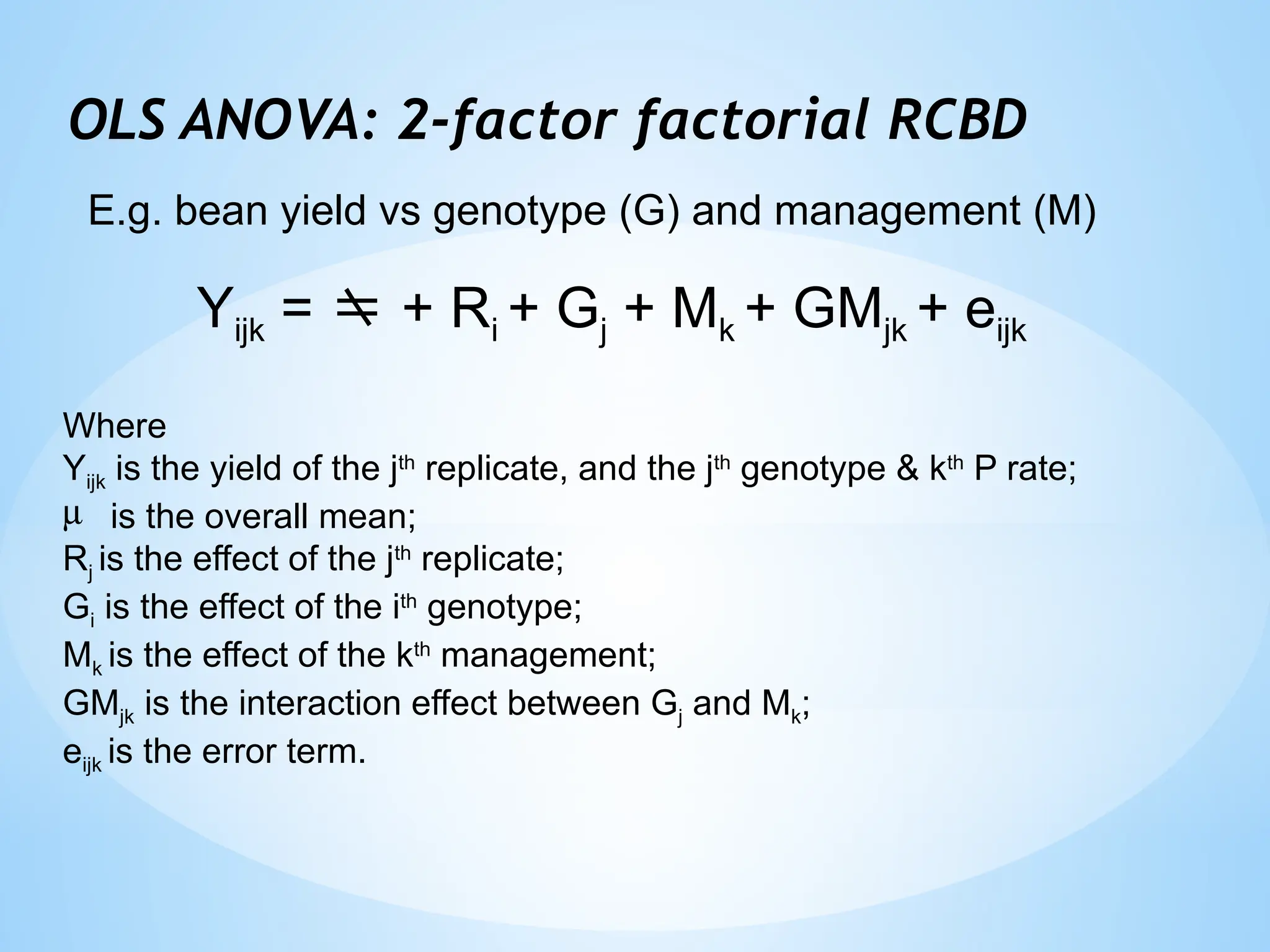
26. OLS ANOVA: 2-factor factorial RCBD
Yijk =  + Ri + Gj + Mk + GMjk + eijk
Where
Yijk is the yield of the jth
replicate, and the jth
genotype & kth
P rate;
m is the overall mean;
Rj is the effect of the jth
replicate;
Gi is the effect of the ith
genotype;
Mk is the effect of the kth
management;
GMjk is the interaction effect between Gj and Mk;
eijk is the error term.
E.g. bean yield vs genotype (G) and management (M)

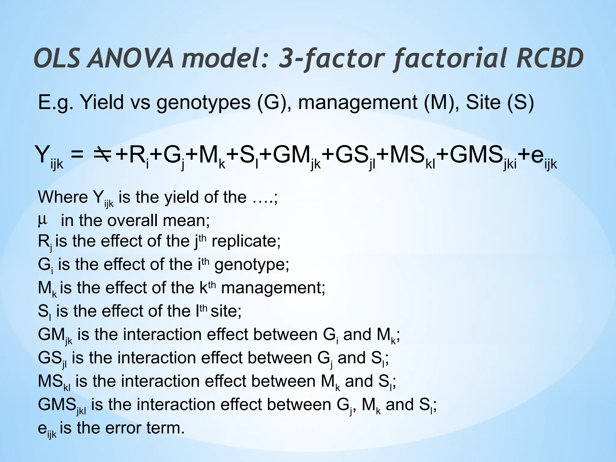
27. Yijk = +Ri+Gj+Mk+Sl+GMjk+GSjl+MSkl+GMSjki+eijk
Where Yijk is the yield of the ….;
m in the overall mean;
Rj is the effect of the jth
replicate;
Gi is the effect of the ith
genotype;
Mk is the effect of the kth
management;
Sl is the effect of the lth
site;
GMjk is the interaction effect between Gi and Mk;
GSjl is the interaction effect between Gj and Sl;
MSkl is the interaction effect between Mk and Sl;
GMSjkl is the interaction effect between Gj, Mk and Sl;
eijk is the error term.
OLS ANOVA model: 3-factor factorial RCBD
E.g. Yield vs genotypes (G), management (M), Site (S)

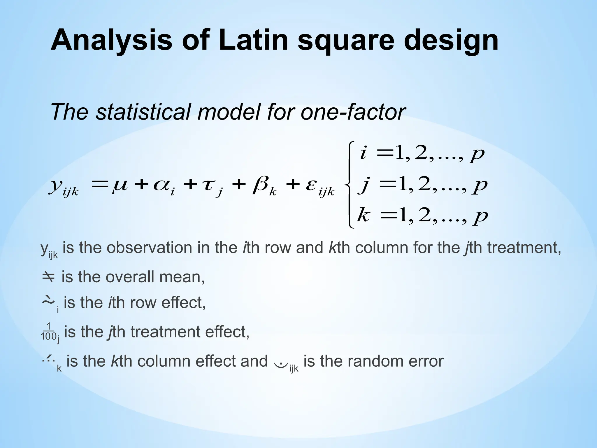
28. yijk
is the observation in the ith row and kth column for the jth treatment,
 is the overall mean,
i
is the ith row effect,
j
is the jth treatment effect,
k
is the kth column effect and ijk
is the random error
1, 2,...,
1, 2,...,
1, 2,...,
ijk i j k ijk
i p
y j p
k p
    



     

 

Analysis of Latin square design
The statistical model for one-factor

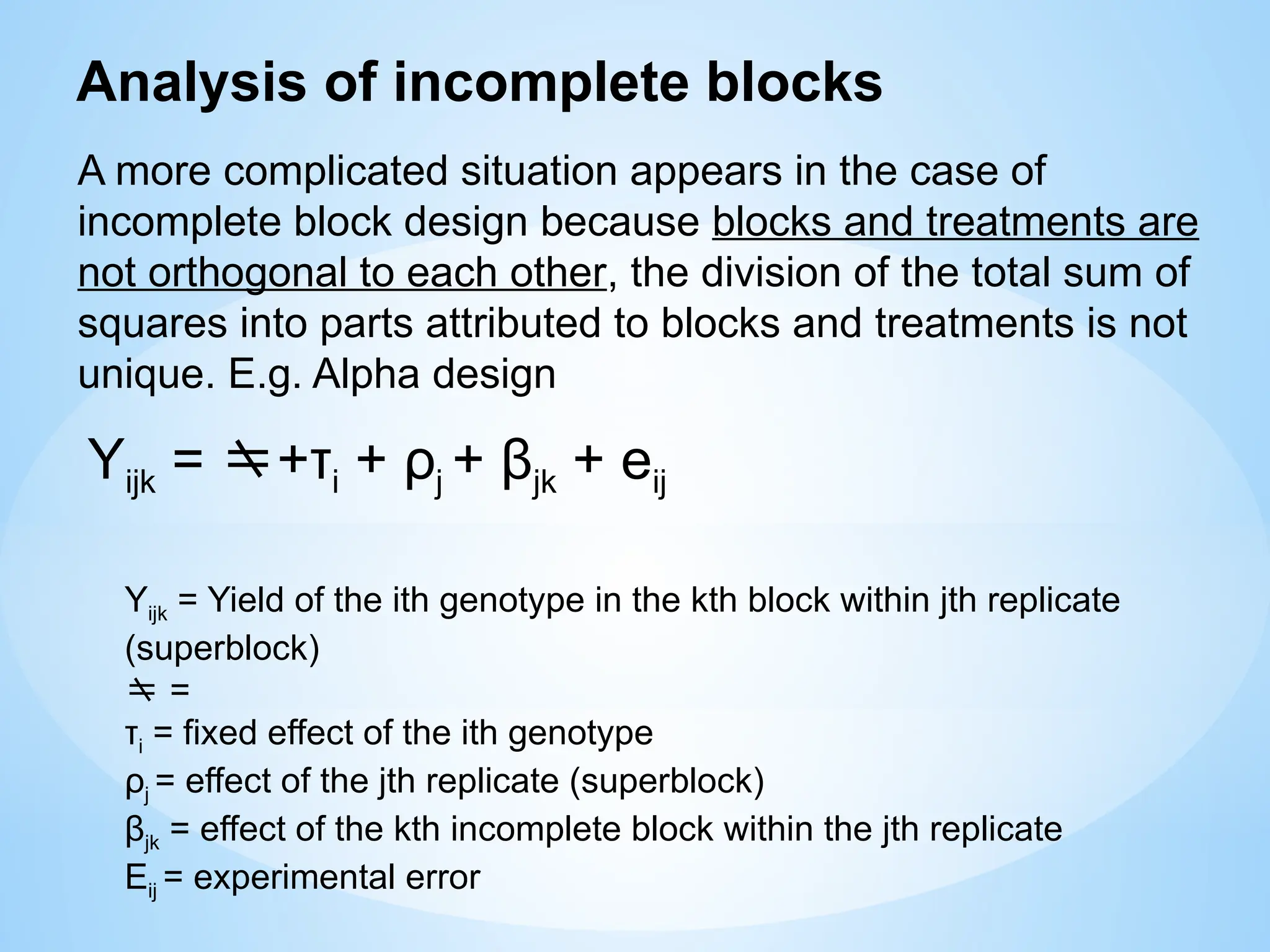
29. A more complicated situation appears in the case of
incomplete block design because blocks and treatments are
not orthogonal to each other, the division of the total sum of
squares into parts attributed to blocks and treatments is not
unique. E.g. Alpha design
Analysis of incomplete blocks
Yijk = +τi + ρj + βjk + eij
Yijk = Yield of the ith genotype in the kth block within jth replicate
(superblock)
 =
τi = fixed effect of the ith genotype
ρj = effect of the jth replicate (superblock)
βjk = effect of the kth incomplete block within the jth replicate
Eij = experimental error

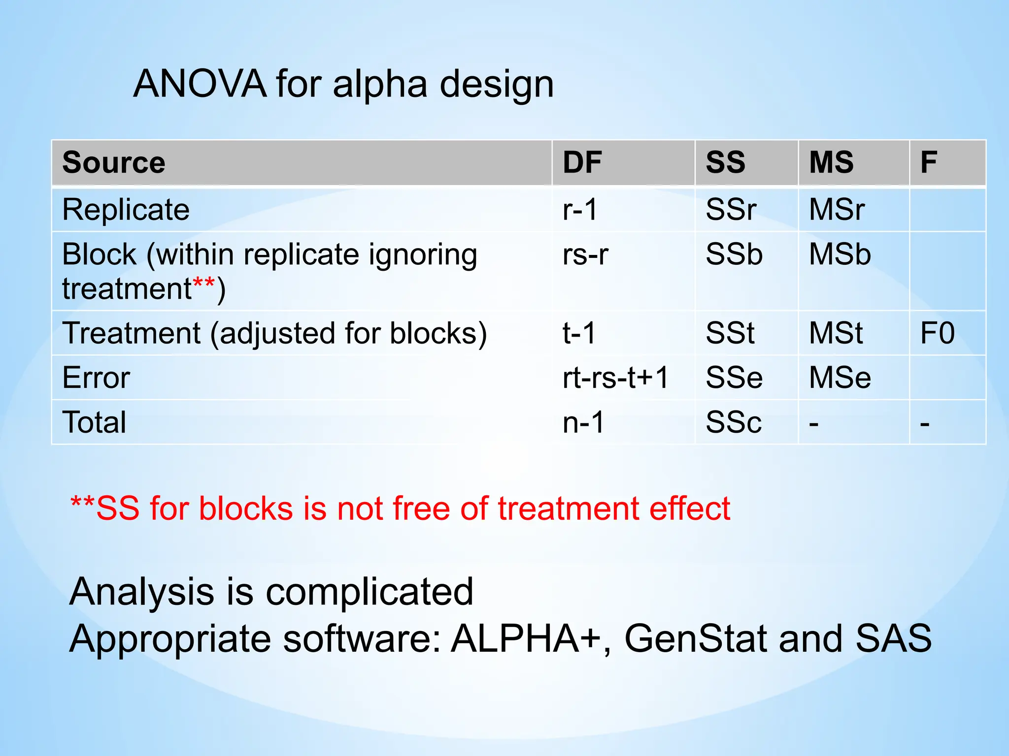
30. Source DF SS MS F
Replicate r-1 SSr MSr
Block (within replicate ignoring
treatment**)
rs-r SSb MSb
Treatment (adjusted for blocks) t-1 SSt MSt F0
Error rt-rs-t+1 SSe MSe
Total n-1 SSc - -
ANOVA for alpha design
Analysis is complicated
Appropriate software: ALPHA+, GenStat and SAS
**SS for blocks is not free of treatment effect

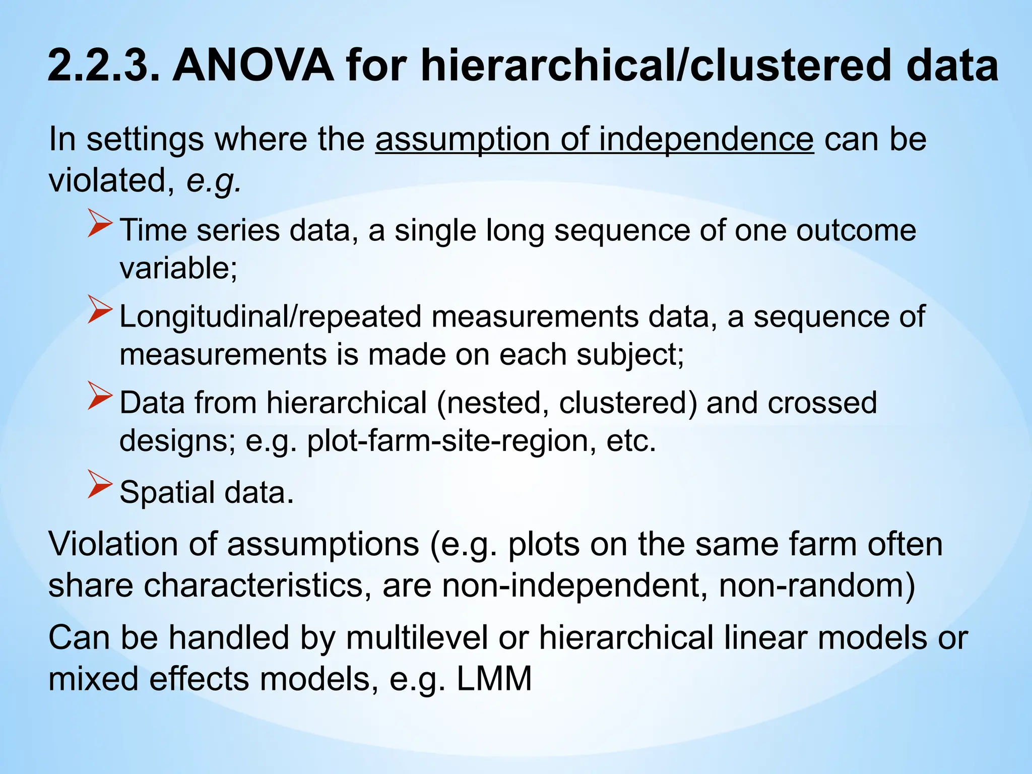
31. 2.2.3. ANOVA for hierarchical/clustered data
In settings where the assumption of independence can be
violated, e.g.
Time series data, a single long sequence of one outcome
variable;
Longitudinal/repeated measurements data, a sequence of
measurements is made on each subject;
Data from hierarchical (nested, clustered) and crossed
designs; e.g. plot-farm-site-region, etc.
Spatial data.
Violation of assumptions (e.g. plots on the same farm often
share characteristics, are non-independent, non-random)
Can be handled by multilevel or hierarchical linear models or
mixed effects models, e.g. LMM

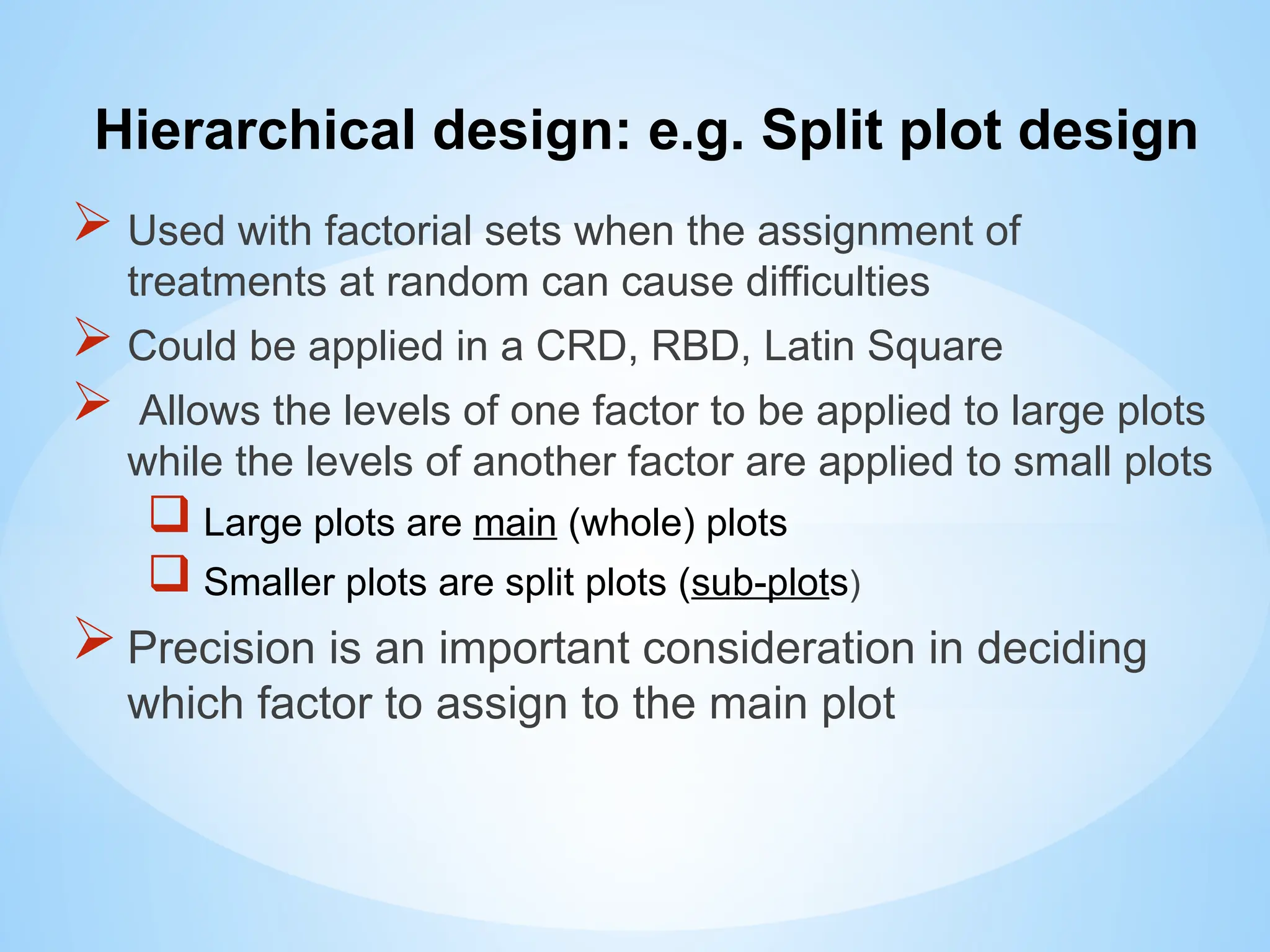
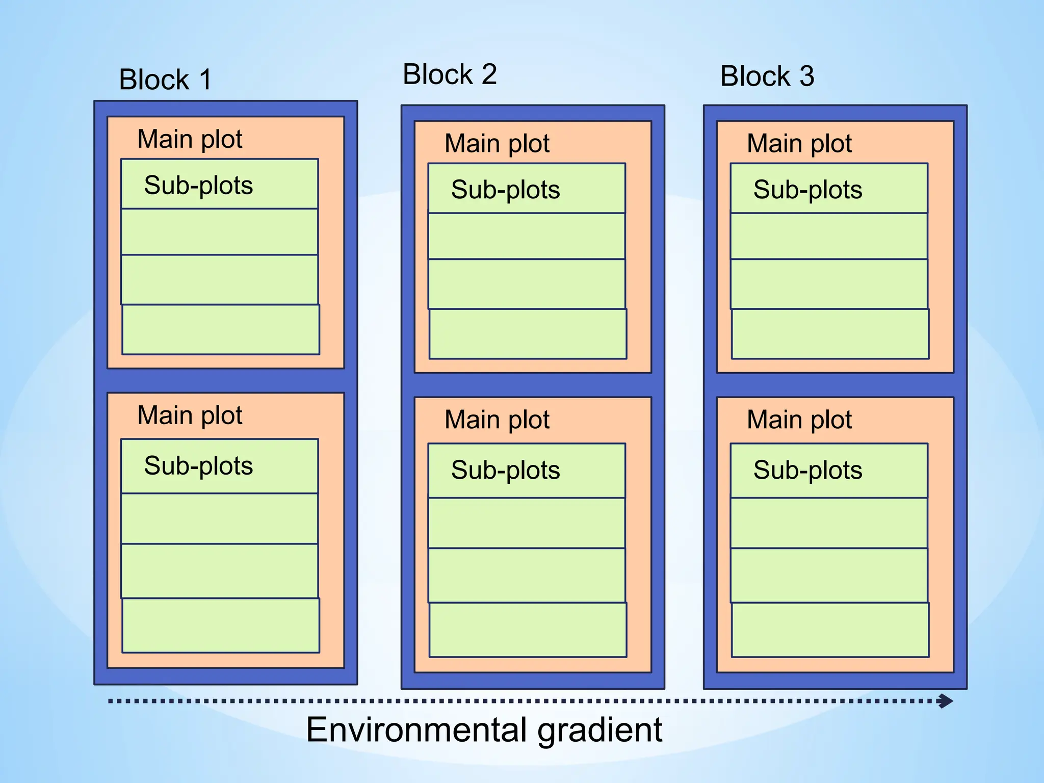
32. Hierarchical design: e.g. Split plot design
 Used with factorial sets when the assignment of
treatments at random can cause difficulties
 Could be applied in a CRD, RBD, Latin Square
 Allows the levels of one factor to be applied to large plots
while the levels of another factor are applied to small plots
 Large plots are main (whole) plots
 Smaller plots are split plots (sub-plots)
Precision is an important consideration in deciding
which factor to assign to the main plot

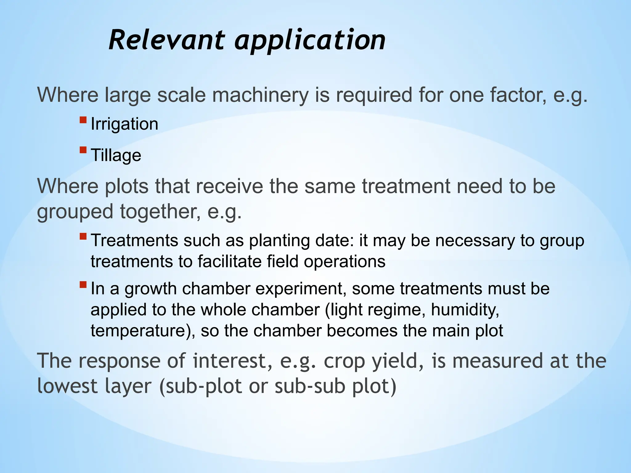
33. Relevant application
Where large scale machinery is required for one factor, e.g.
Irrigation
Tillage
Where plots that receive the same treatment need to be
grouped together, e.g.
Treatments such as planting date: it may be necessary to group
treatments to facilitate field operations
In a growth chamber experiment, some treatments must be
applied to the whole chamber (light regime, humidity,
temperature), so the chamber becomes the main plot
The response of interest, e.g. crop yield, is measured at the
lowest layer (sub-plot or sub-sub plot)

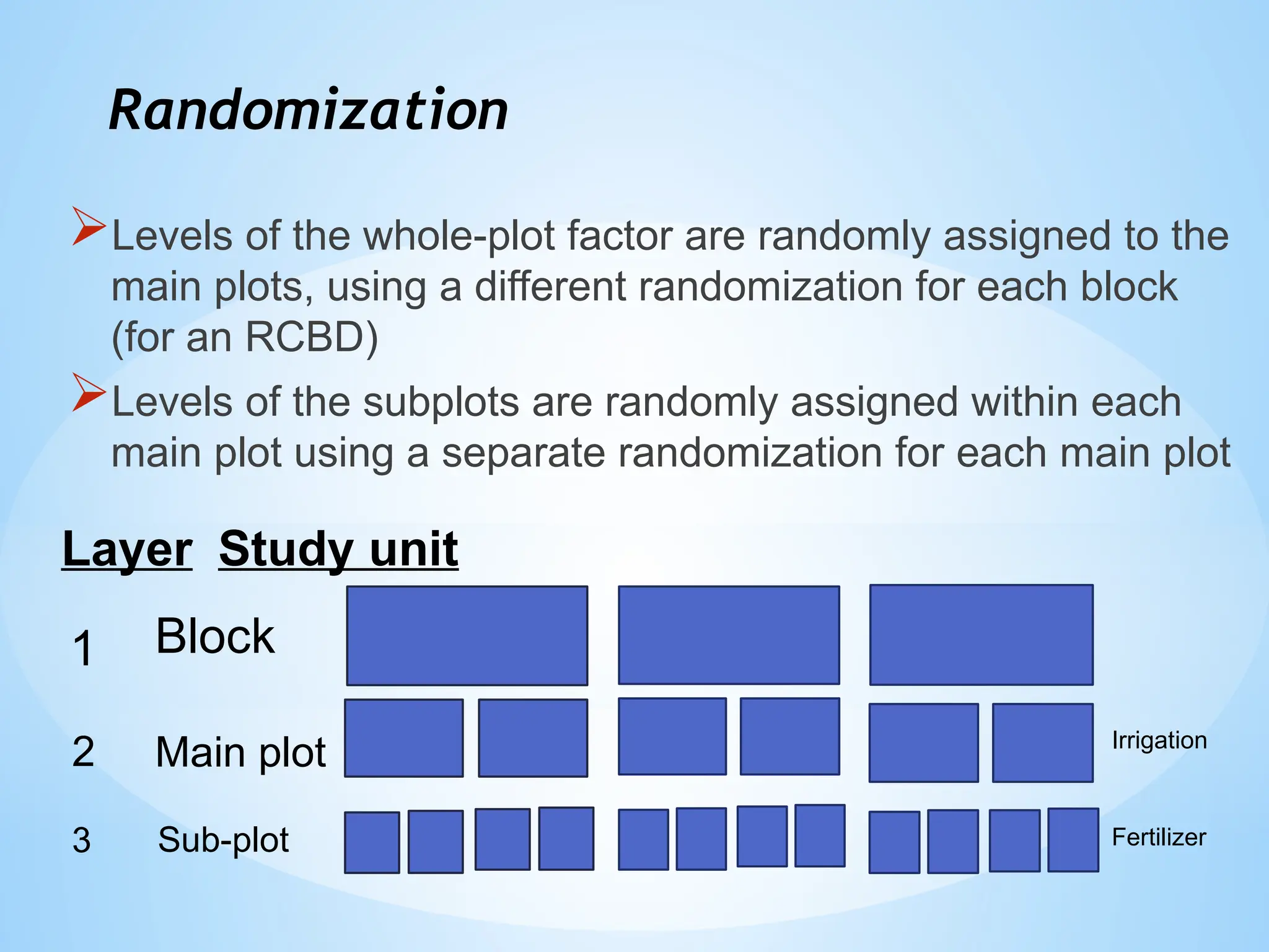
34. Randomization
Levels of the whole-plot factor are randomly assigned to the
main plots, using a different randomization for each block
(for an RCBD)
Levels of the subplots are randomly assigned within each
main plot using a separate randomization for each main plot
Layer
1 Block
2
Study unit
Main plot
Sub-plot
3
Irrigation
Fertilizer

35. Block 1
Sub-plots
Main plot
Sub-plots
Main plot
Sub-plots
Main plot
Sub-plots
Main plot
Block 2 Block 3
Sub-plots
Main plot
Sub-plots
Main plot
Environmental gradient

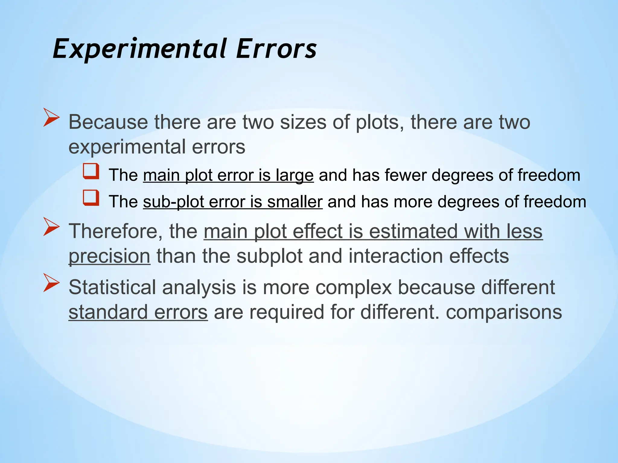
36. Experimental Errors
 Because there are two sizes of plots, there are two
experimental errors
 The main plot error is large and has fewer degrees of freedom
 The sub-plot error is smaller and has more degrees of freedom
 Therefore, the main plot effect is estimated with less
precision than the subplot and interaction effects
 Statistical analysis is more complex because different
standard errors are required for different. comparisons

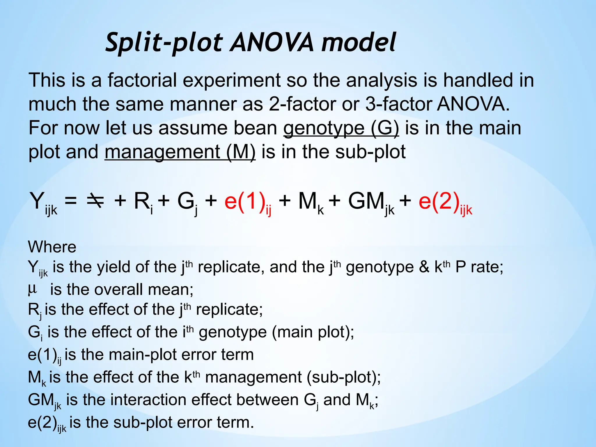
37. Split-plot ANOVA model
Yijk =  + Ri + Gj + e(1)ij + Mk + GMjk + e(2)ijk
Where
Yijk is the yield of the jth
replicate, and the jth
genotype & kth
P rate;
m is the overall mean;
Rj is the effect of the jth
replicate;
Gi is the effect of the ith
genotype (main plot);
e(1)ij is the main-plot error term
Mk is the effect of the kth
management (sub-plot);
GMjk is the interaction effect between Gj and Mk;
e(2)ijk is the sub-plot error term.
This is a factorial experiment so the analysis is handled in
much the same manner as 2-factor or 3-factor ANOVA.
For now let us assume bean genotype (G) is in the main
plot and management (M) is in the sub-plot

38. Source DF SS MS F
Total rgm-1 SST
Block (R) r-1 SSR MSR FR
Genotype g-1 SSG MSG FG
Error(1) (r-1)(g-1) SSE1 MSEA Main plot error
Management m-1 SSM MSM FM
GxM (g-1)(m-1) SSGM MSGM FGM
Error(2) g(r-1)(m-1) SSE2 MSEb Subplot error
Error (1): Block x Genotype
Error (2): Block x Genotype x Management
Split-plot ANOVA table

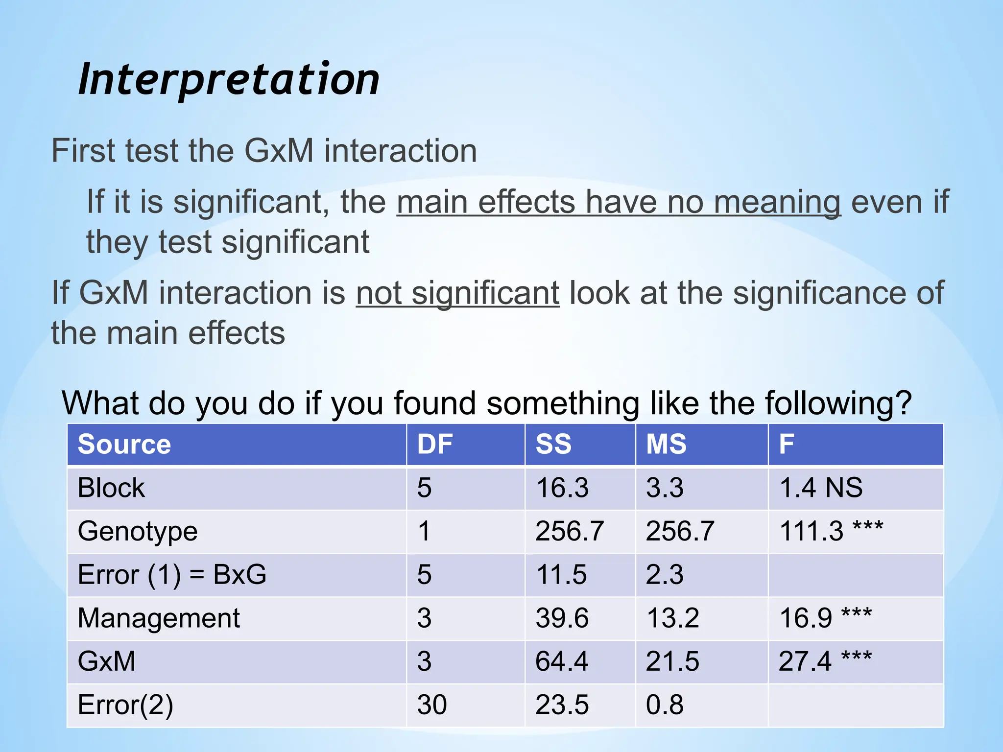
39. Interpretation
First test the GxM interaction
If it is significant, the main effects have no meaning even if
they test significant
If GxM interaction is not significant look at the significance of
the main effects
Source DF SS MS F
Block 5 16.3 3.3 1.4 NS
Genotype 1 256.7 256.7 111.3 ***
Error (1) = BxG 5 11.5 2.3
Management 3 39.6 13.2 16.9 ***
GxM 3 64.4 21.5 27.4 ***
Error(2) 30 23.5 0.8
What do you do if you found something like the following?

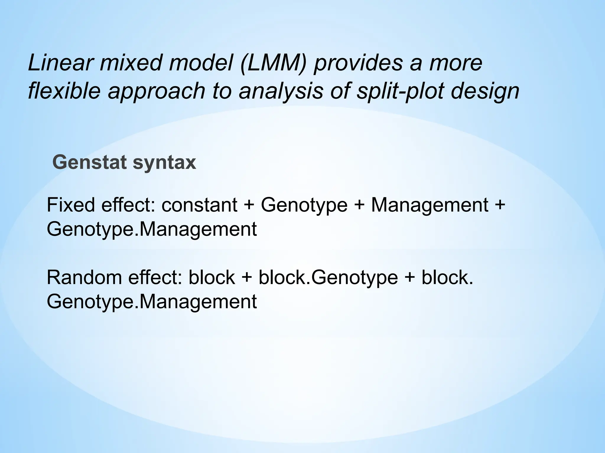
40. Genstat syntax
Fixed effect: constant + Genotype + Management +
Genotype.Management
Random effect: block + block.Genotype + block.
Genotype.Management
Linear mixed model (LMM) provides a more
flexible approach to analysis of split-plot design

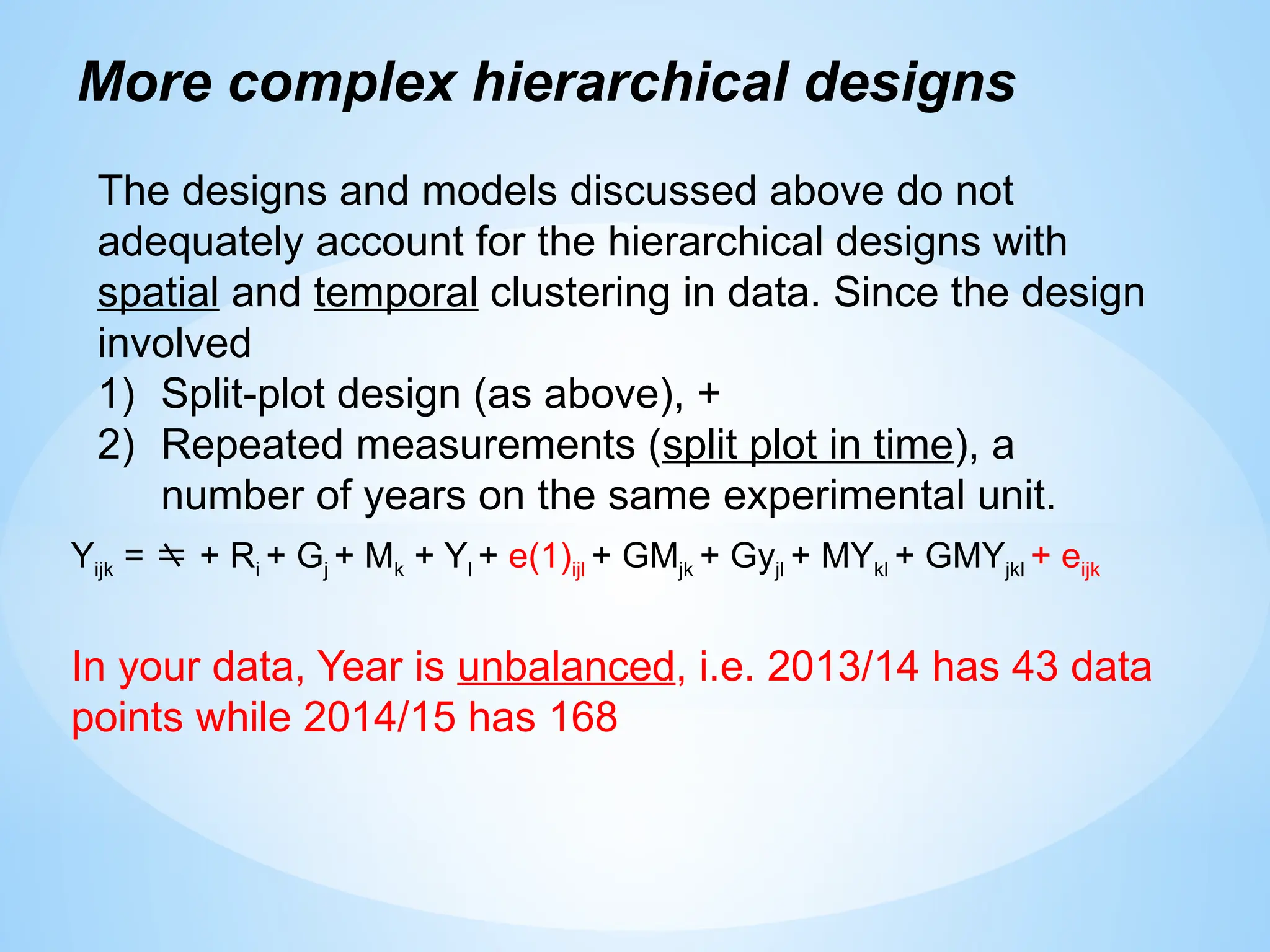
41. More complex hierarchical designs
The designs and models discussed above do not
adequately account for the hierarchical designs with
spatial and temporal clustering in data. Since the design
involved
1) Split-plot design (as above), +
2) Repeated measurements (split plot in time), a
number of years on the same experimental unit.
Yijk =  + Ri + Gj + Mk + Yl + e(1)ijl + GMjk + Gyjl + MYkl + GMYjkl + eijk
In your data, Year is unbalanced, i.e. 2013/14 has 43 data
points while 2014/15 has 168

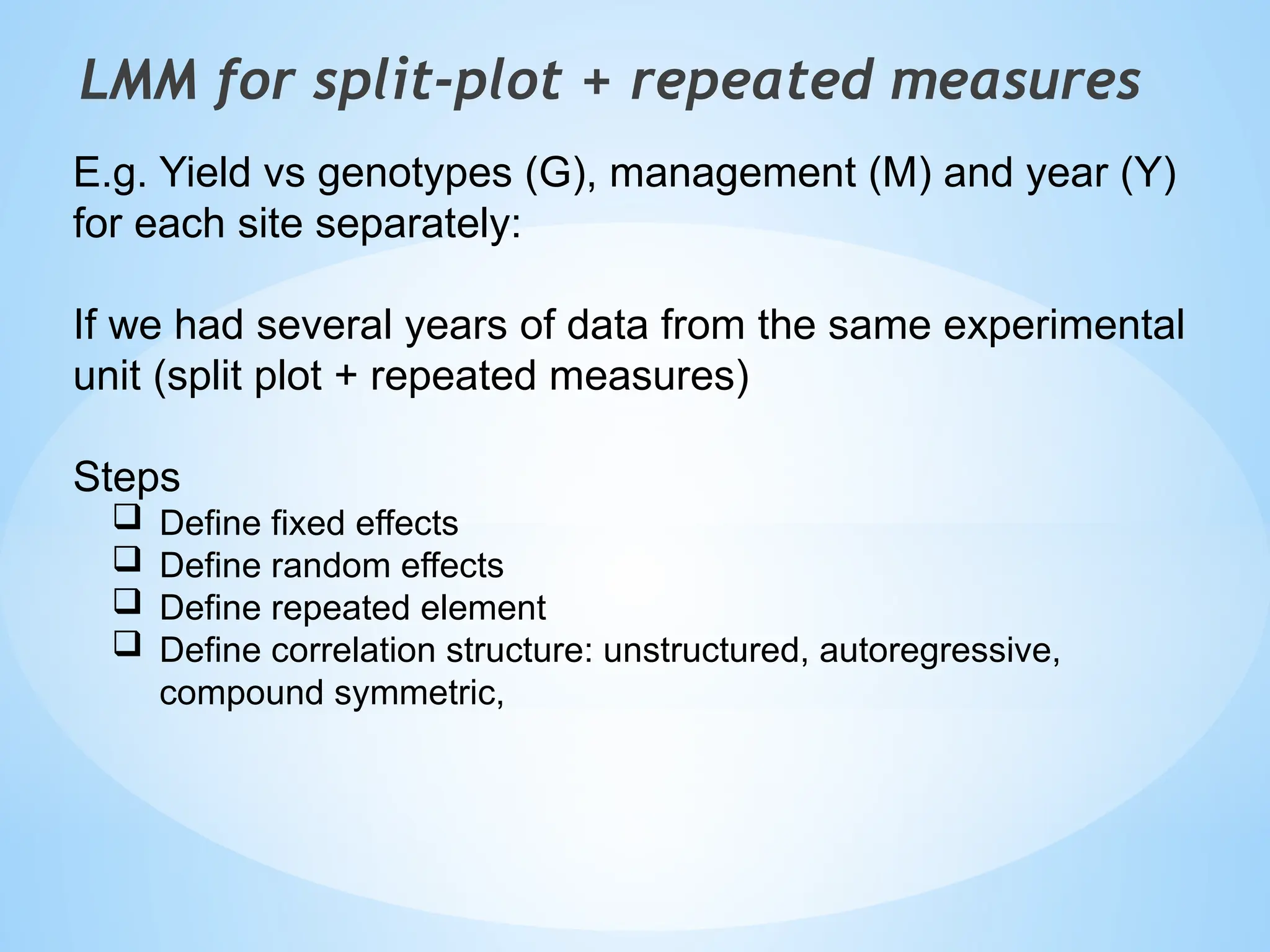
42. LMM for split-plot + repeated measures
E.g. Yield vs genotypes (G), management (M) and year (Y)
for each site separately:
If we had several years of data from the same experimental
unit (split plot + repeated measures)
Steps
 Define fixed effects
 Define random effects
 Define repeated element
 Define correlation structure: unstructured, autoregressive,
compound symmetric,

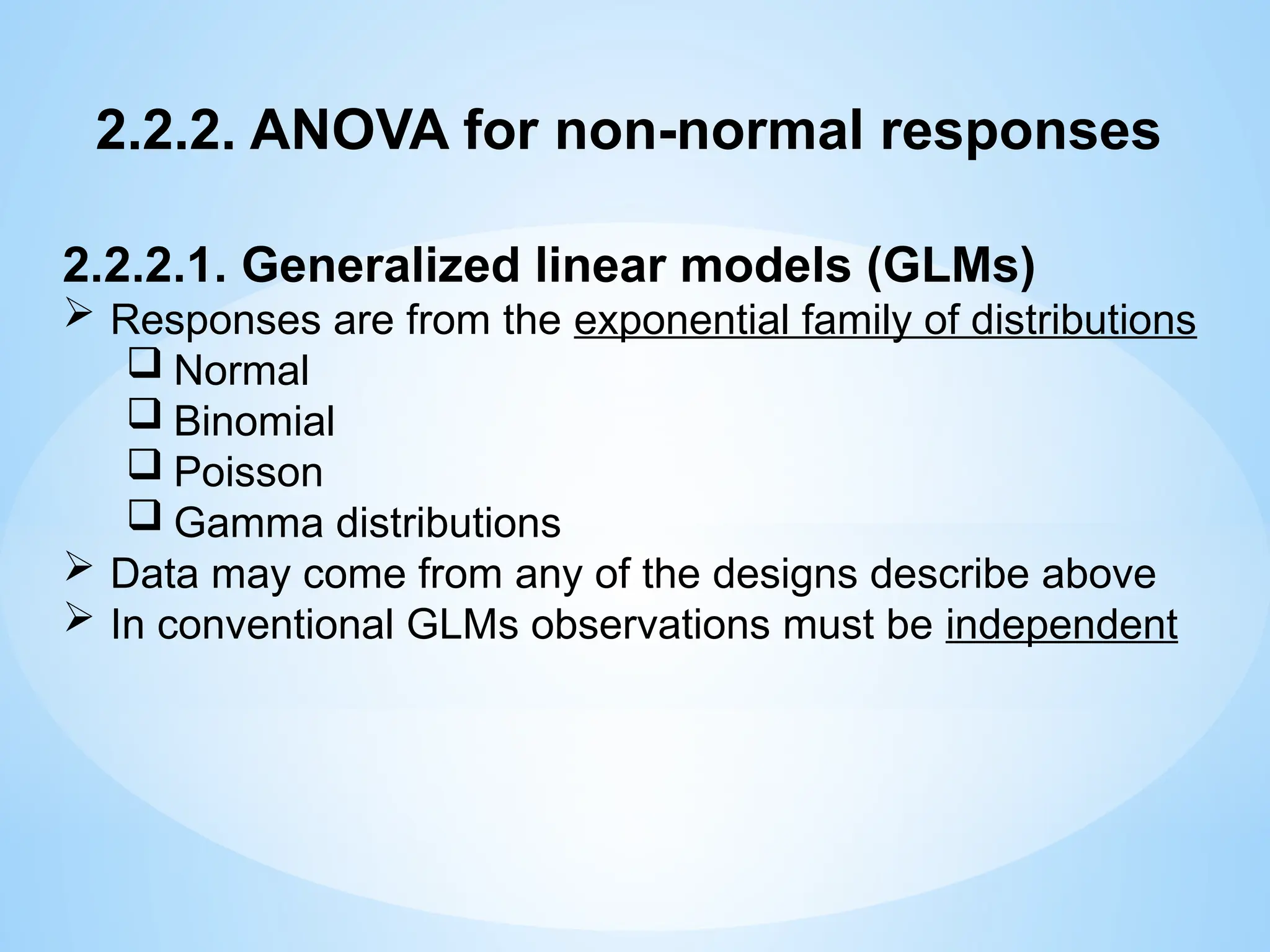
43. 2.2.2. ANOVA for non-normal responses
2.2.2.1. Generalized linear models (GLMs)
 Responses are from the exponential family of distributions
 Normal
 Binomial
 Poisson
 Gamma distributions
 Data may come from any of the designs describe above
 In conventional GLMs observations must be independent

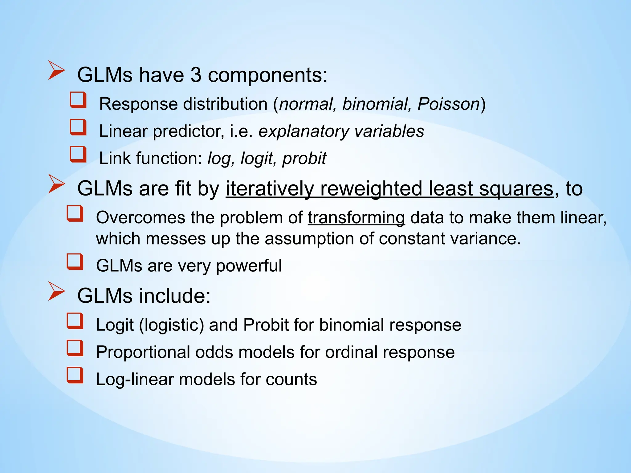
44.  GLMs have 3 components:
 Response distribution (normal, binomial, Poisson)
 Linear predictor, i.e. explanatory variables
 Link function: log, logit, probit
 GLMs are fit by iteratively reweighted least squares, to
 Overcomes the problem of transforming data to make them linear,
which messes up the assumption of constant variance.
 GLMs are very powerful
 GLMs include:
 Logit (logistic) and Probit for binomial response
 Proportional odds models for ordinal response
 Log-linear models for counts

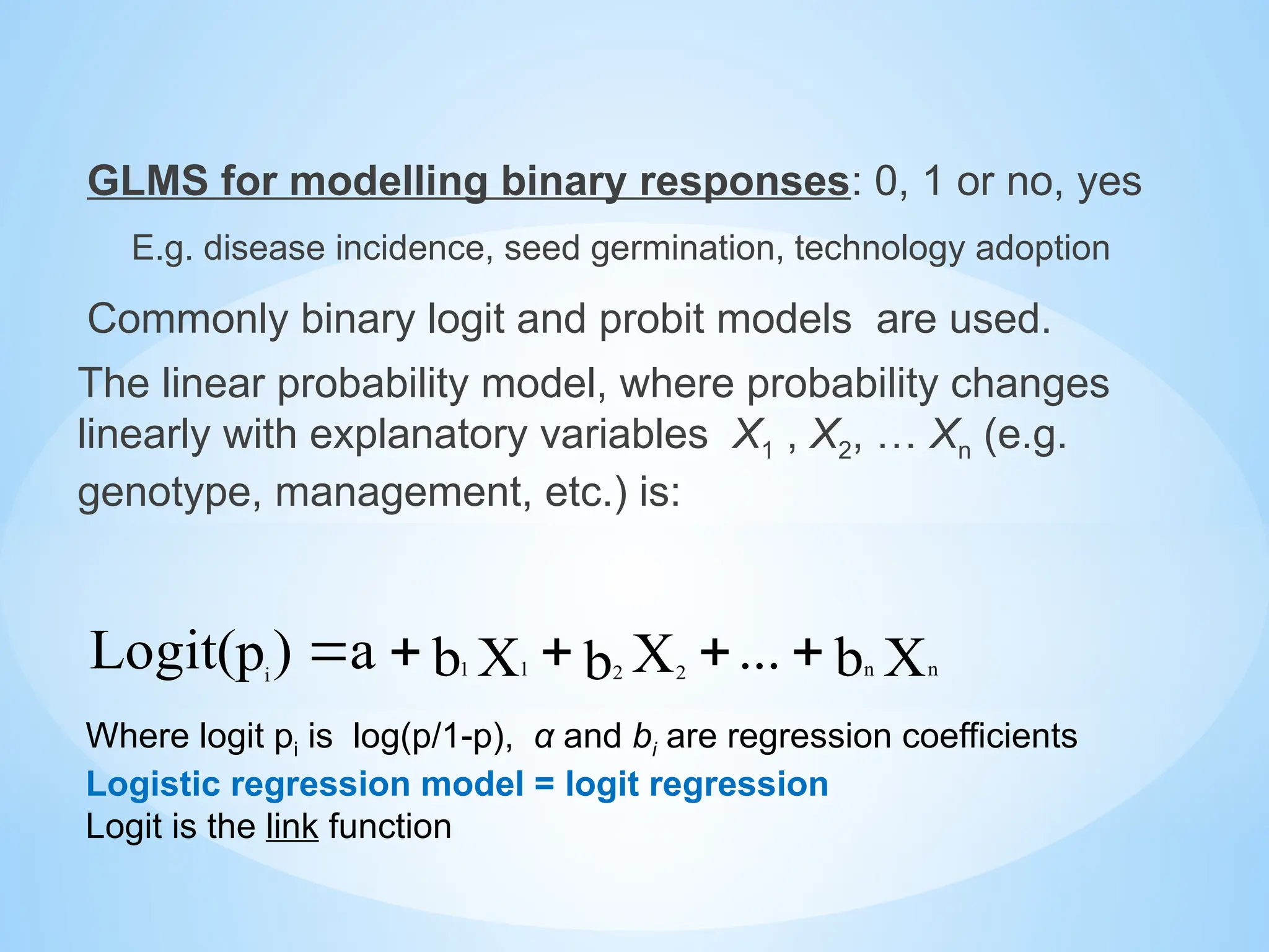
45. GLMS for modelling binary responses: 0, 1 or no, yes
E.g. disease incidence, seed germination, technology adoption
Commonly binary logit and probit models are used.
The linear probability model, where probability changes
linearly with explanatory variables X1 , X2, … Xn (e.g.
genotype, management, etc.) is:
Where logit pi is log(p/1-p), α and bi are regression coefficients
Logistic regression model = logit regression
Logit is the link function
X
b
...
X
b
X
b
a
)
p
Logit( n
n
2 2
1
1
i






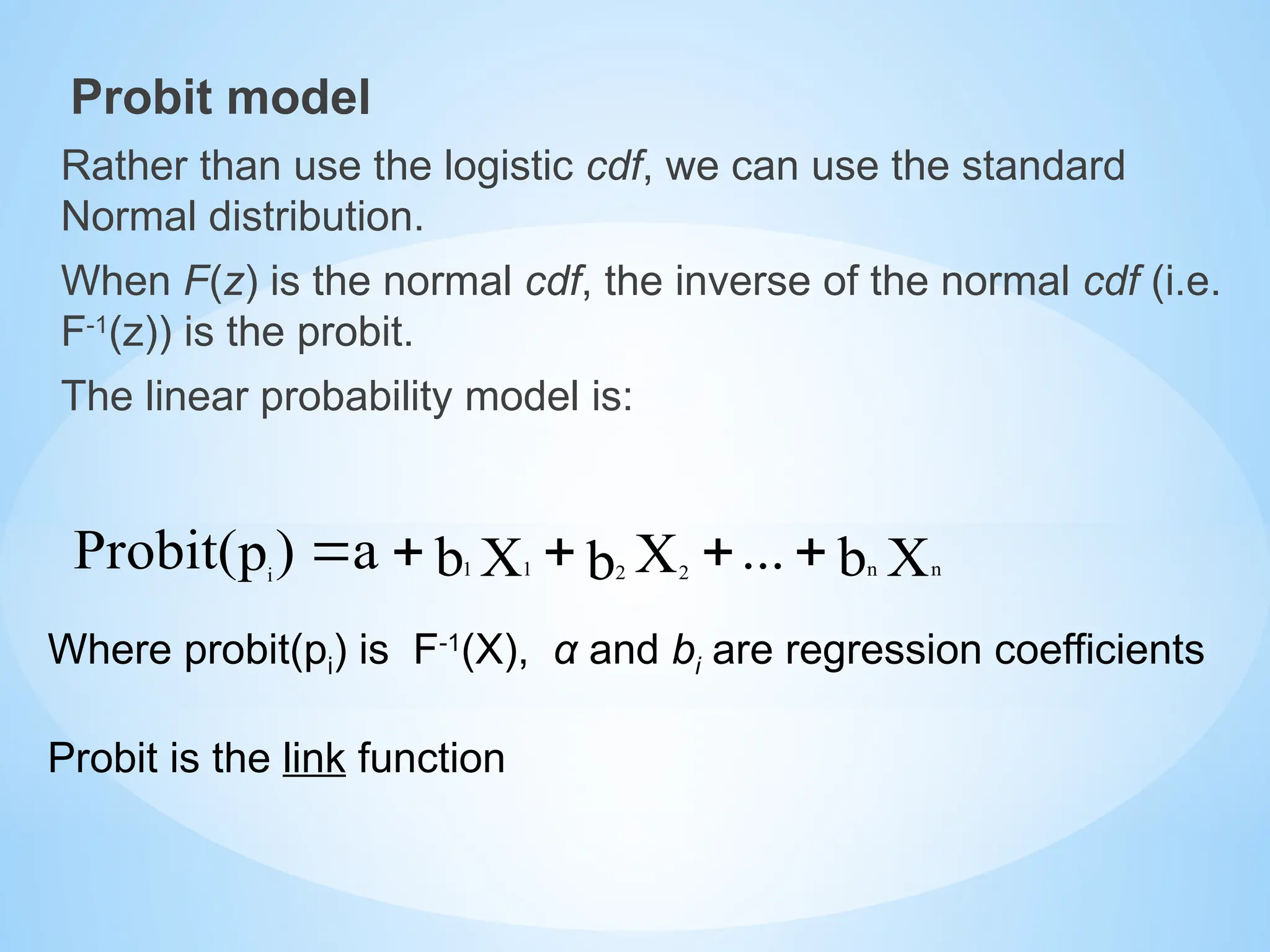
46. Probit model
Rather than use the logistic cdf, we can use the standard
Normal distribution.
When F(z) is the normal cdf, the inverse of the normal cdf (i.e.
F-1
(z)) is the probit.
The linear probability model is:
Where probit(pi) is F-1
(X), α and bi are regression coefficients
Probit is the link function
X
b
...
X
b
X
b
a
)
p
Probit( n
n
2 2
1
1
i






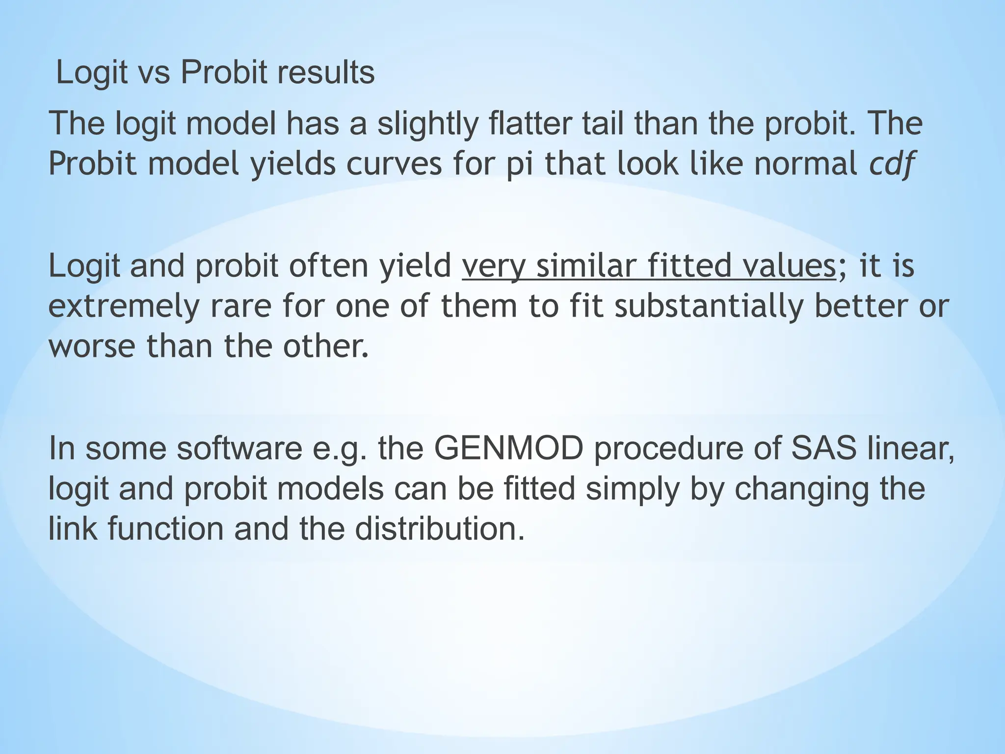
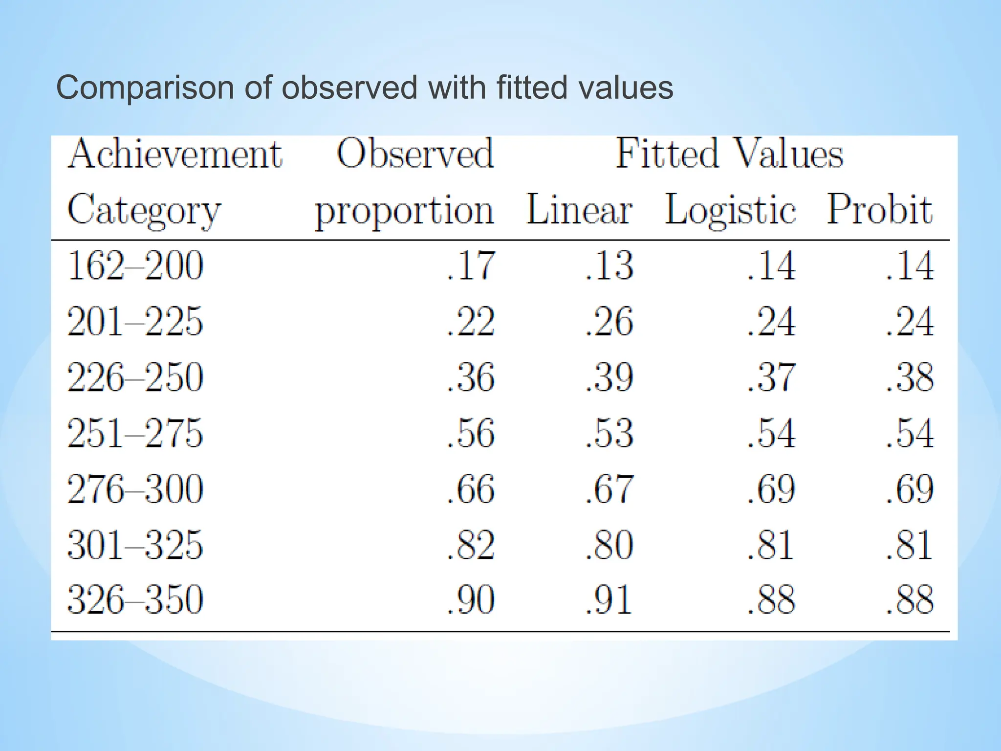
47. Logit vs Probit results
The logit model has a slightly flatter tail than the probit. The
Probit model yields curves for pi that look like normal cdf
Logit and probit often yield very similar fitted values; it is
extremely rare for one of them to fit substantially better or
worse than the other.
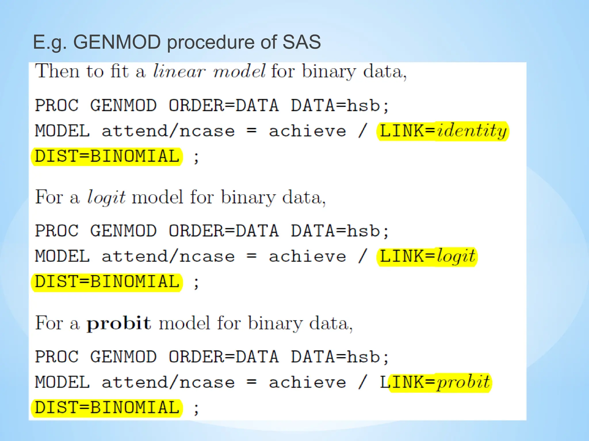
In some software e.g. the GENMOD procedure of SAS linear,
logit and probit models can be fitted simply by changing the
link function and the distribution.

48. E.g. GENMOD procedure of SAS

49. Comparison of observed with fitted values

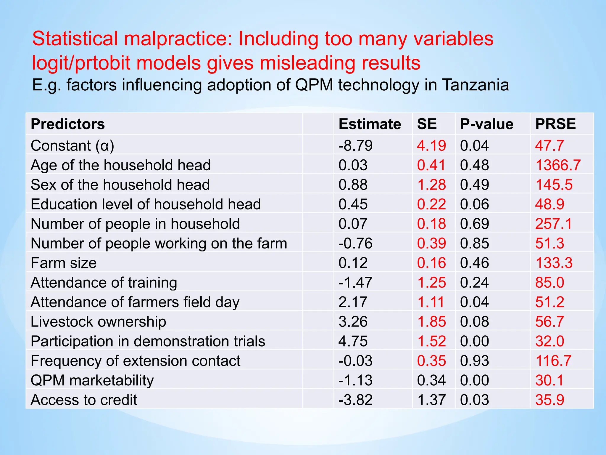
50. Predictors Estimate SE P-value PRSE
Constant (α) -8.79 4.19 0.04 47.7
Age of the household head 0.03 0.41 0.48 1366.7
Sex of the household head 0.88 1.28 0.49 145.5
Education level of household head 0.45 0.22 0.06 48.9
Number of people in household 0.07 0.18 0.69 257.1
Number of people working on the farm -0.76 0.39 0.85 51.3
Farm size 0.12 0.16 0.46 133.3
Attendance of training -1.47 1.25 0.24 85.0
Attendance of farmers field day 2.17 1.11 0.04 51.2
Livestock ownership 3.26 1.85 0.08 56.7
Participation in demonstration trials 4.75 1.52 0.00 32.0
Frequency of extension contact -0.03 0.35 0.93 116.7
QPM marketability -1.13 0.34 0.00 30.1
Access to credit -3.82 1.37 0.03 35.9
Statistical malpractice: Including too many variables
logit/prtobit models gives misleading results
E.g. factors influencing adoption of QPM technology in Tanzania

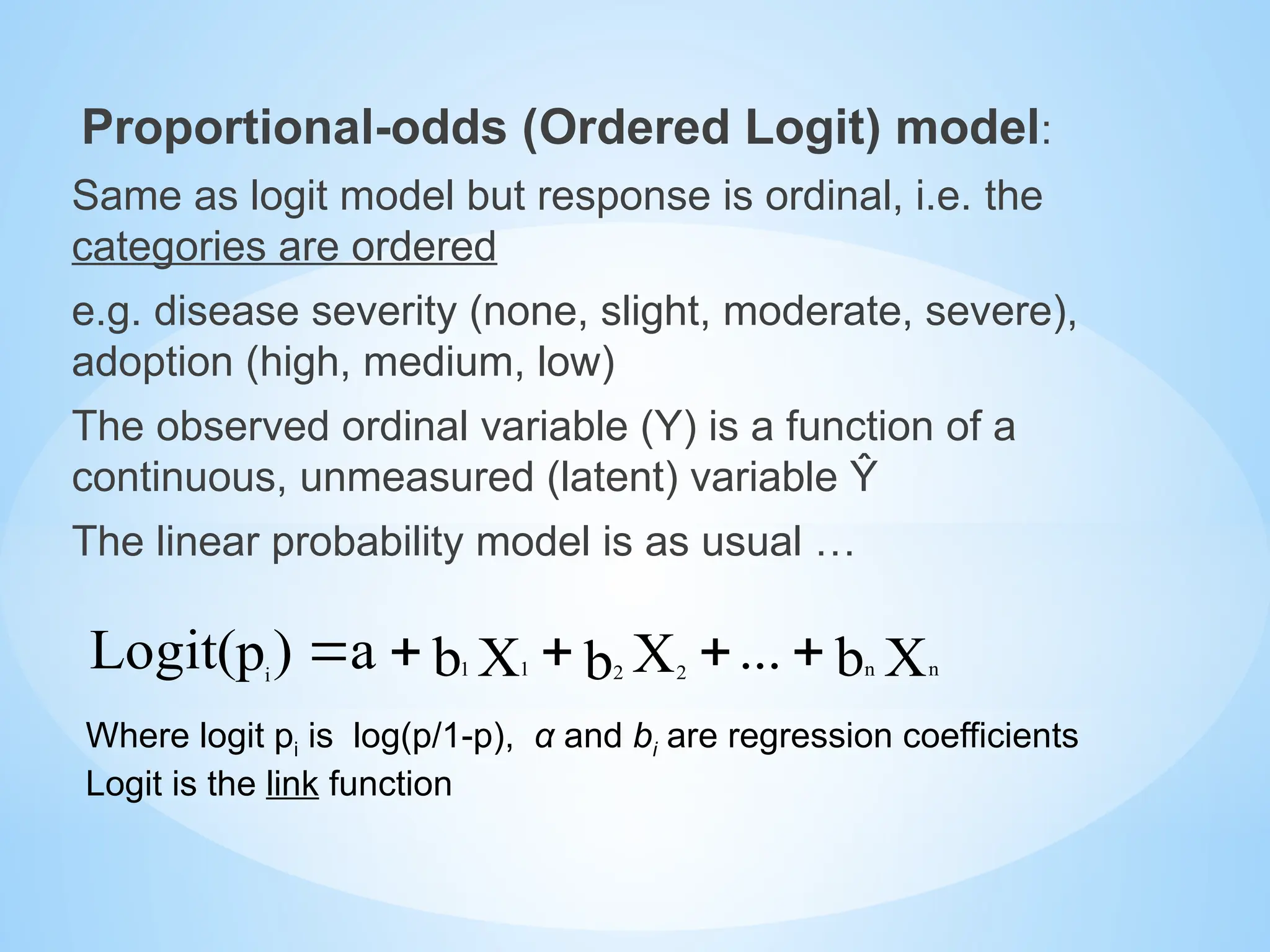
51. Proportional-odds (Ordered Logit) model:
Same as logit model but response is ordinal, i.e. the
categories are ordered
e.g. disease severity (none, slight, moderate, severe),
adoption (high, medium, low)
The observed ordinal variable (Y) is a function of a
continuous, unmeasured (latent) variable Ŷ
The linear probability model is as usual …
Where logit pi is log(p/1-p), α and bi are regression coefficients
Logit is the link function
X
b
...
X
b
X
b
a
)
p
Logit( n
n
2 2
1
1
i






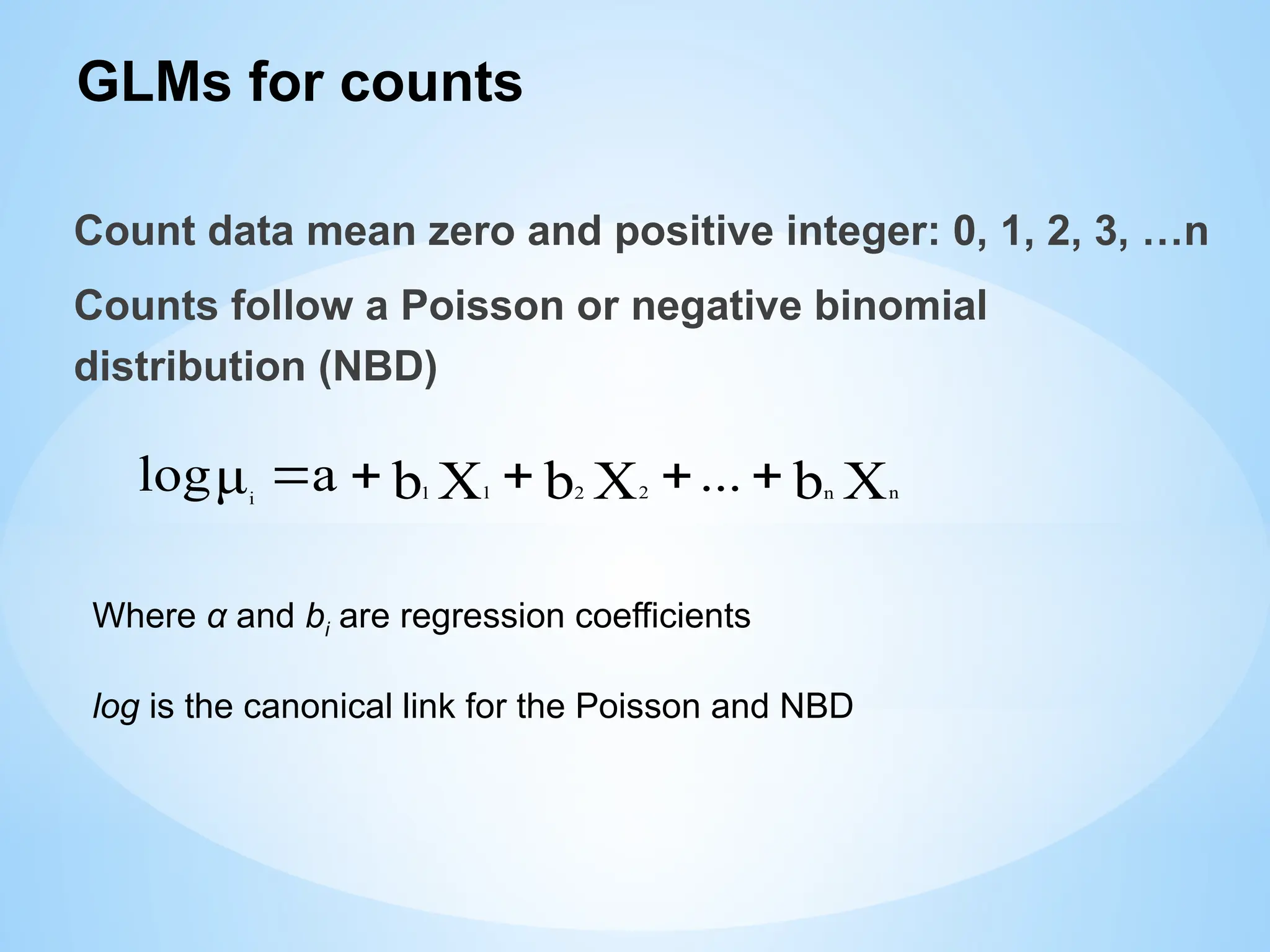
52. GLMs for counts
Count data mean zero and positive integer: 0, 1, 2, 3, …n
Counts follow a Poisson or negative binomial
distribution (NBD)
Where α and bi are regression coefficients
log is the canonical link for the Poisson and NBD
X
b
X
b
X
b
μ n
n
2
2
1
1
i
...
a
log 





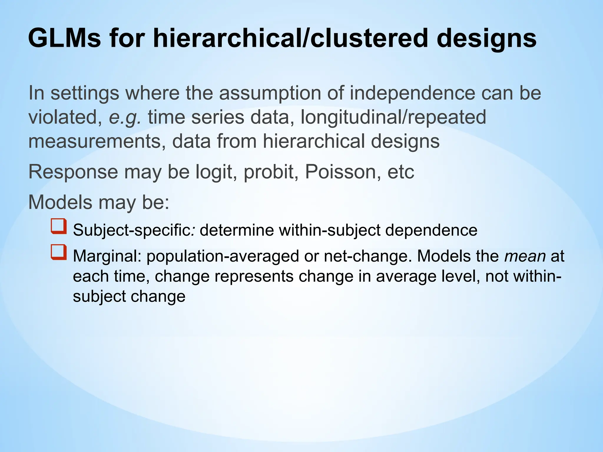
53. GLMs for hierarchical/clustered designs
In settings where the assumption of independence can be
violated, e.g. time series data, longitudinal/repeated
measurements, data from hierarchical designs
Response may be logit, probit, Poisson, etc
Models may be:
 Subject-specific: determine within-subject dependence
 Marginal: population-averaged or net-change. Models the mean at
each time, change represents change in average level, not within-
subject change

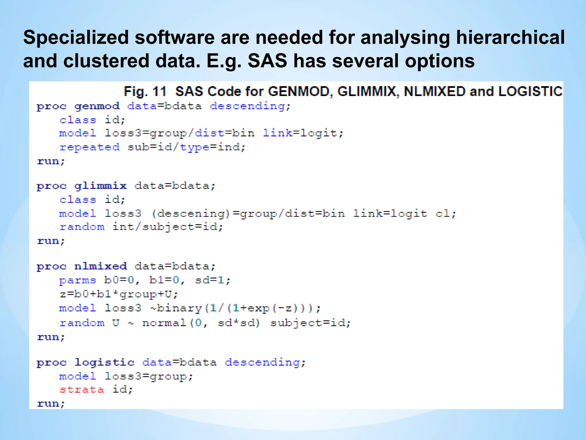
54. Specialized software are needed for analysing hierarchical
and clustered data. E.g. SAS has several options

55. When can you combine data?
 If the design/management of experiments is the same;
 If the same thing was measured on all sites and/or years;
 If all sites and/or years have equal sample sizes;
Combining can have surprising effects; e.g. Simpsons paradox
2.3. Multi-site and multi-year data analysis
If the goal of the research is to establish that a particular
treatment has broad applicability, assessing variability
across sites and years may provide insight into the
conditions under which the treatment is effective.

56. Common approaches:
1. Mega-analysis: Combining all data into a single analysis
This does not need new methods or concepts. But first
 Test whether the site or year by treatment interaction is
significant
 Linear mixed models (LMMs) with site or site x
treatment as a random effect
2. Stability analysis: different regression techniques
3. Meta analysis:
This requires calculating effect sizes, i.e. summary statistics
such as mean differences between treatment and control.
Linear mixed models (LMMs)

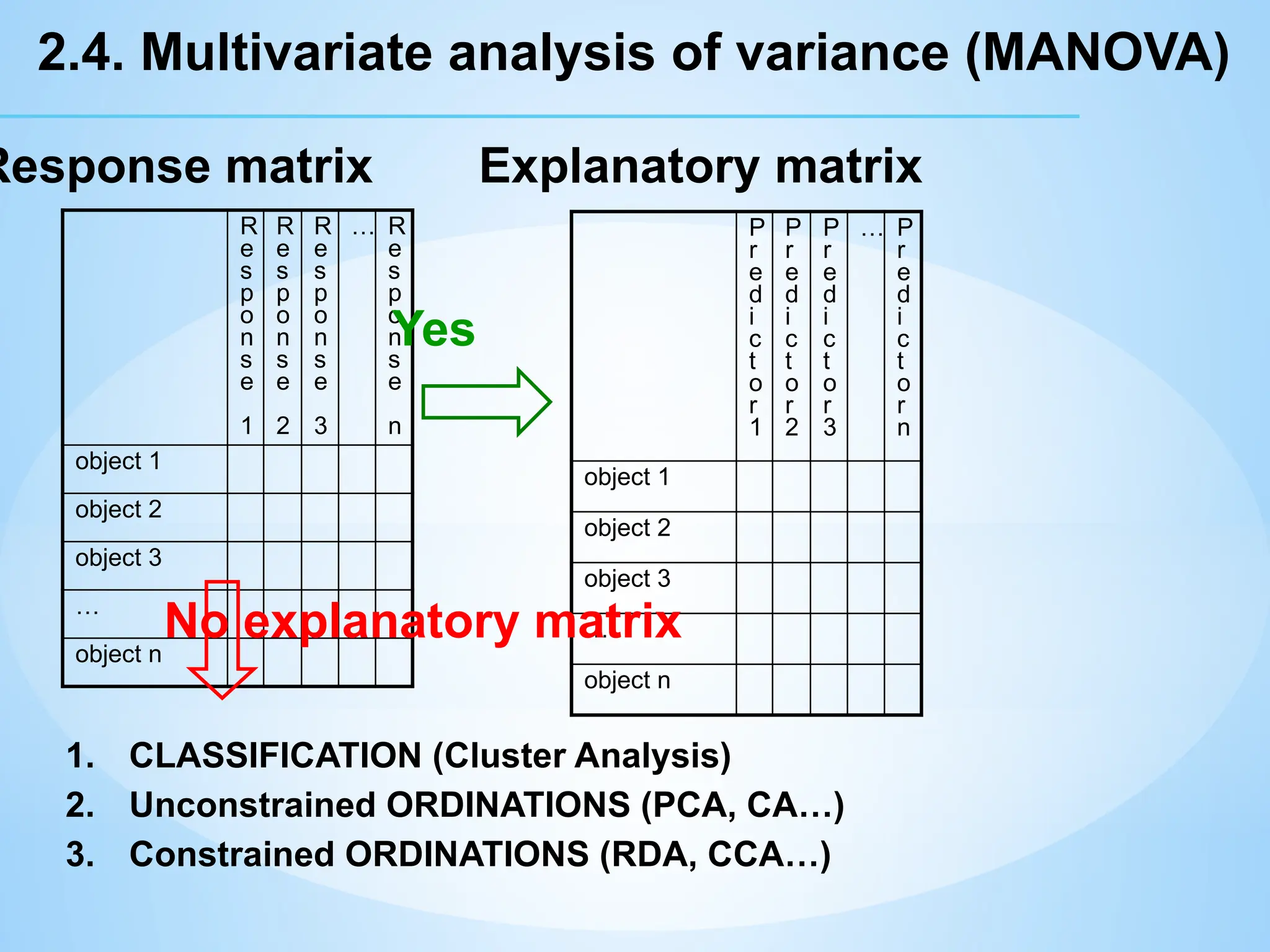
57. R
e
s
p
o
n
s
e
1
R
e
s
p
o
n
s
e
2
R
e
s
p
o
n
s
e
3
… R
e
s
p
o
n
s
e
n
object 1
object 2
object 3
…
object n
Response matrix
P
r
e
d
i
c
t
o
r
1
P
r
e
d
i
c
t
o
r
2
P
r
e
d
i
c
t
o
r
3
… P
r
e
d
i
c
t
o
r
n
object 1
object 2
object 3
…
object n
Explanatory matrix
Yes
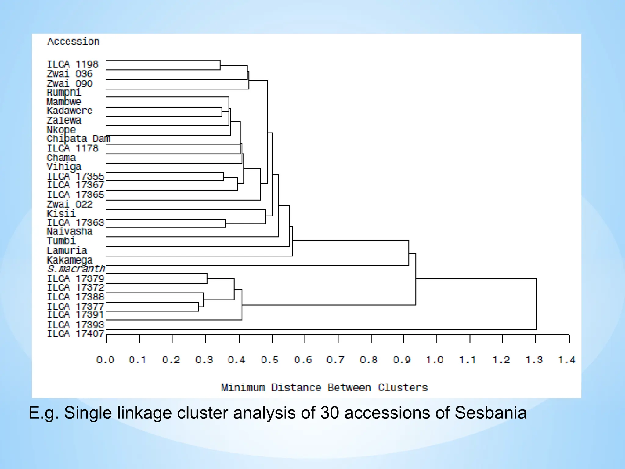
1. CLASSIFICATION (Cluster Analysis)
2. Unconstrained ORDINATIONS (PCA, CA…)
3. Constrained ORDINATIONS (RDA, CCA…)
No explanatory matrix
2.4. Multivariate analysis of variance (MANOVA)

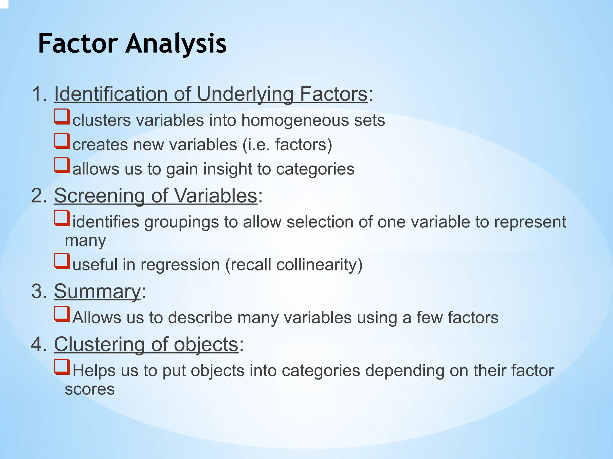
58. Factor Analysis
1. Identification of Underlying Factors:
clusters variables into homogeneous sets
creates new variables (i.e. factors)
allows us to gain insight to categories
2. Screening of Variables:
identifies groupings to allow selection of one variable to represent
many
useful in regression (recall collinearity)
3. Summary:
Allows us to describe many variables using a few factors
4. Clustering of objects:
Helps us to put objects into categories depending on their factor
scores

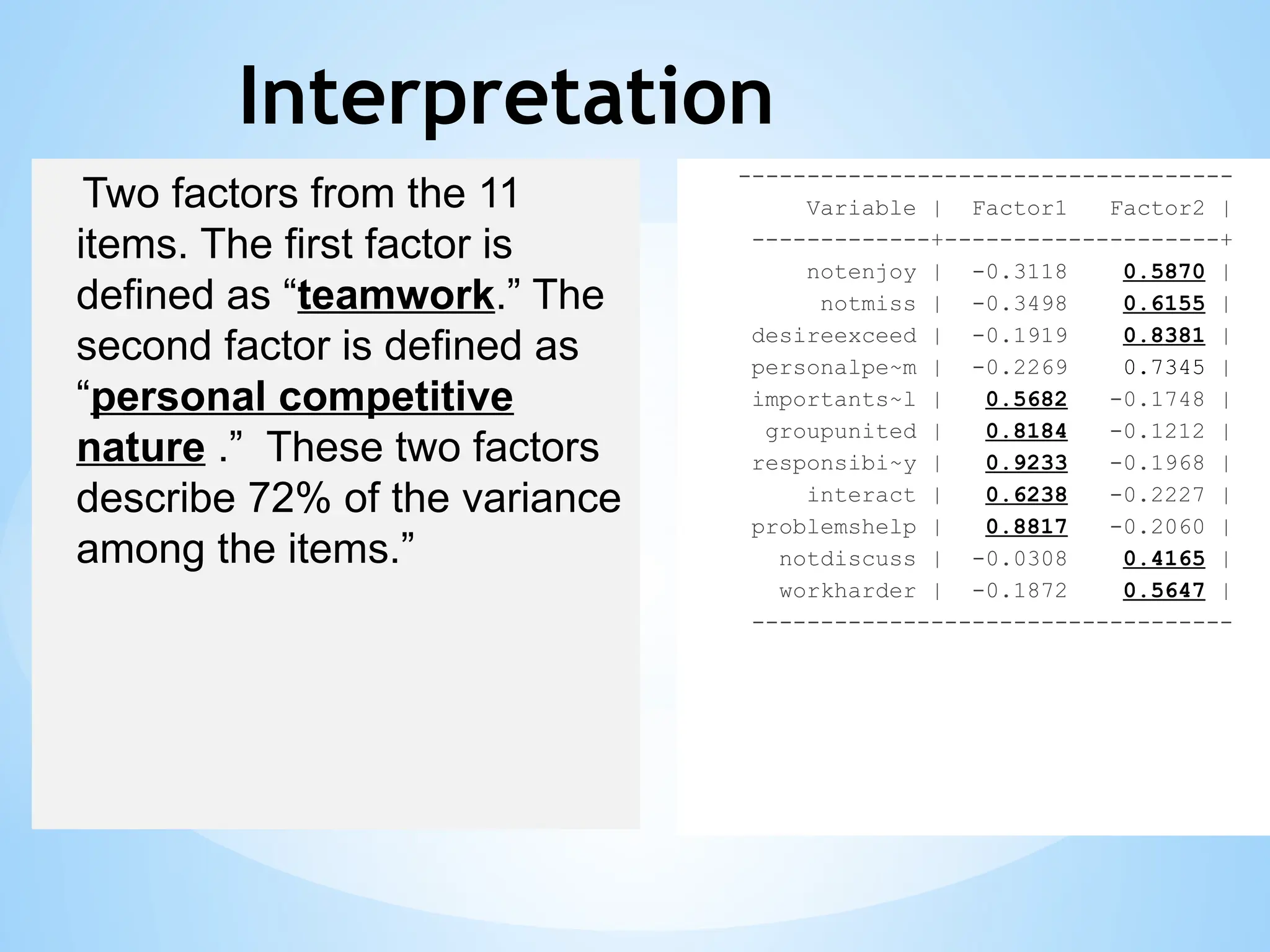
59. Interpretation
------------------------------------
Variable | Factor1 Factor2 |
-------------+--------------------+
notenjoy | -0.3118 0.5870 |
notmiss | -0.3498 0.6155 |
desireexceed | -0.1919 0.8381 |
personalpe~m | -0.2269 0.7345 |
importants~l | 0.5682 -0.1748 |
groupunited | 0.8184 -0.1212 |
responsibi~y | 0.9233 -0.1968 |
interact | 0.6238 -0.2227 |
problemshelp | 0.8817 -0.2060 |
notdiscuss | -0.0308 0.4165 |
workharder | -0.1872 0.5647 |
-----------------------------------
Two factors from the 11
items. The first factor is
defined as “teamwork.” The
second factor is defined as
“personal competitive
nature .” These two factors
describe 72% of the variance
among the items.”

60. Distance-dissimilarity
The most natural dissimilarity measure is the Euclidean distance
(distance in variable space - each variable is an axis)
Dissimilarity
Sp
1
Sp 2 Sp
3
object 1
object 2
object3
o
bj
e
ct
1
o
bj
e
ct
2
o
bj
e
ct
3
… o
bj
e
ct
n
object 1
object 2
object 3
…
object n
One value for
each possible pair of objects
Euclidean distance: [Σ(xi j-xi k)2
]0.5
Indices: Jaccard index, Manhattan, Bray-Curtis, Morisita

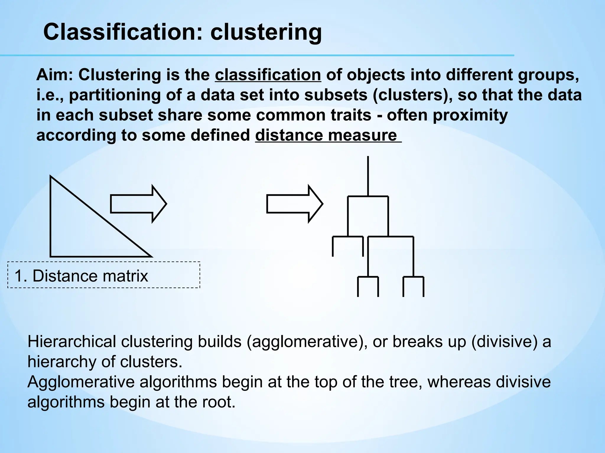
61. Classification: clustering
Aim: Clustering is the classification of objects into different groups,
i.e., partitioning of a data set into subsets (clusters), so that the data
in each subset share some common traits - often proximity
according to some defined distance measure
1. Distance matrix
Hierarchical clustering builds (agglomerative), or breaks up (divisive) a
hierarchy of clusters.
Agglomerative algorithms begin at the top of the tree, whereas divisive
algorithms begin at the root.

62. E.g. Single linkage cluster analysis of 30 accessions of Sesbania

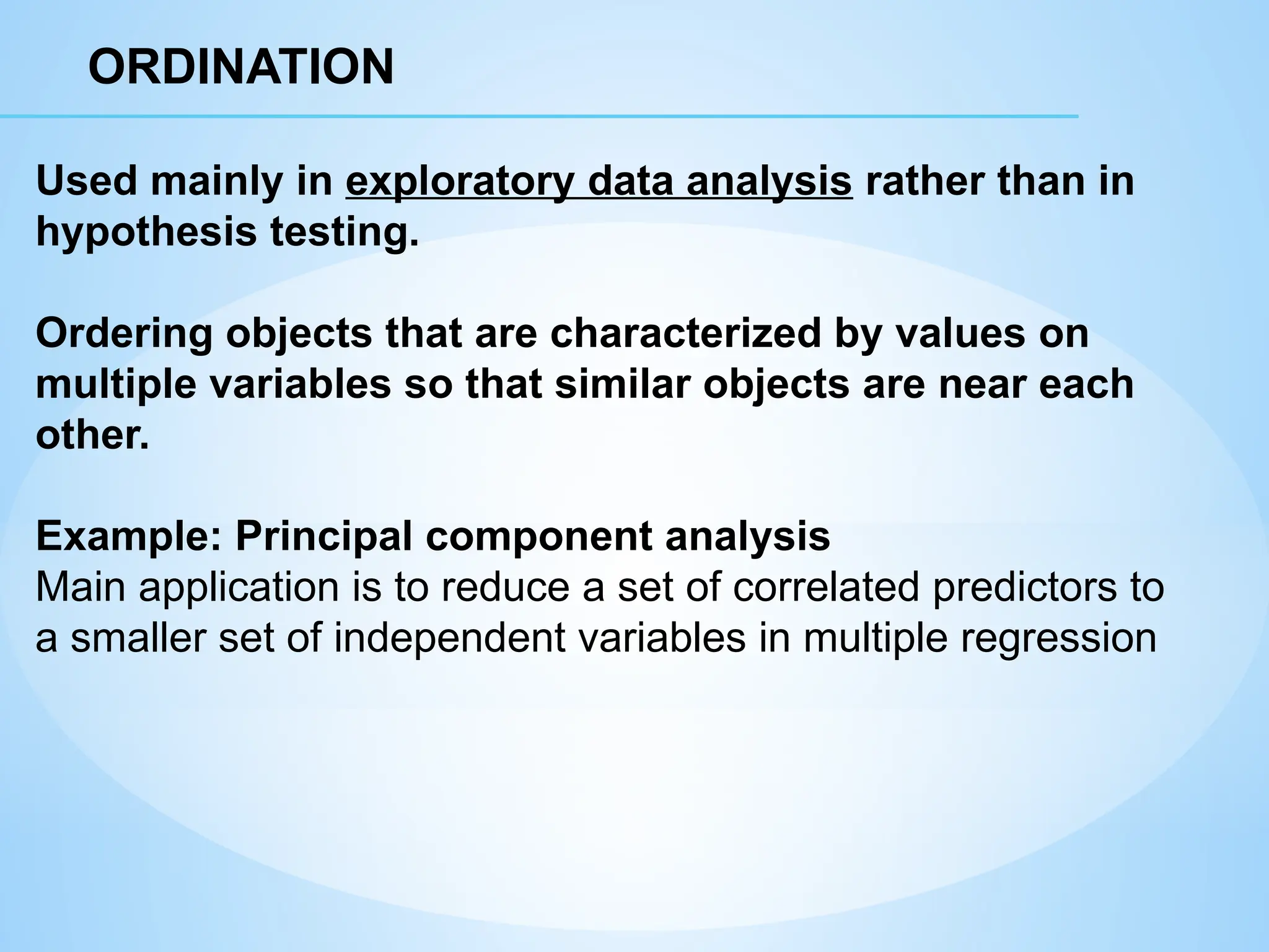
63. ORDINATION
Used mainly in exploratory data analysis rather than in
hypothesis testing.
Ordering objects that are characterized by values on
multiple variables so that similar objects are near each
other.
Example: Principal component analysis
Main application is to reduce a set of correlated predictors to
a smaller set of independent variables in multiple regression

64. 3. COMMUNICATING UNCERTAINTY
Each study has several sources of uncertainty
-Environment, operator, equipment, mathematical models
The value of any study lies in the appropriate communication
of the outcome and the uncertainty surrounding the
outcome
Communicating uncertainty appropriately will:
 guide decision-making
 increase credibility and confidence in the work
Report responsibly; present and discuss the:
 outcomes and a measures of dispersion (Xbest ± CL);
 risks and the relevance to users;
 limitations of the study and caveats;
 unknowns and implications for future research.