This document discusses modeling the relationship between corporate debt and equity returns over the credit cycle using a regime switching model. It first provides background on theories of the debt-equity relationship and evidence that their returns often diverge. It then introduces the concept of a "leverage clock" where debt and equity risk premiums move together in some parts of the credit cycle but diverge in others. The document outlines previous attempts at regime switching models to capture this cycle but notes limitations. It aims to develop a new model to identify historical credit cycle regimes and predict future monthly transitions between states.

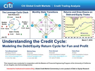
1. Understanding the Credit Cycle:
The Leverage Cycle Clock Monthly State Transitions
Terry Benzschawel
Managing Director
Credit Quantitative Analysis
terry.l.benzschawel@citi.com
+1 212-723-1464
Modeling the Debt/Equity Return Cycle for Fun and Profit
Mahima Garg
Associate
Credit Quantitative Analysis
mahima1.garg@citi.com
+1 212-723-1381
Prem Dwivedi
Associate
Credit Quantitative Analysis
prem.suarav.dwivedi@citi.com
+91 224-277-5042
Claire Ruan
Analyst
Credit Quantitative Analysis
claire.ruan@citi.com
+1 212-723-3262
Citi Global Credit Markets  Credit Trading Analysis
March 7, 2016
Intended for Institutional Investors Only | Global Credit Market Commentary is not a product of Debt or Equity Research
This research was conducted in cooperation with the Masters of Financial Engineering Program at the University of California
at Los Angeles (see Acknowledgements)
Jan-16
Returns and Draw-Downs on
Debt-and-Equity Trades

2. 2
1. Introduction and Background
2. The Leverage Clock and Regime Switching Model
3. Quantifying the Debt-Equity Credit Cycle
4. Predicting Monthly Regime States Transitions
5. Out-of-Sample Testing
A1: Acknowledgments
A2: Disclaimer

3. 3
Objectives
The purpose of this report is to understand and model the dynamics of divergence
between equity and debt market returns and develop a model to predict those returns.
 In the first portion of the presentation, we seek to understand the theoretical
basis for the divergence between equity and debt returns
─ We begin by describing the corporate leverage cycle which has been hypothesized
to drive divergences between equity and debt returns
─ We next present analyses of risk premia in the equity and debt markets as they
relate to the corporate leverage cycle
─ The section concludes with a brief description of regime switching models that have
been proposed to describe equity and debt market dynamics
 An important part of the presentation is the identification assignment of
historical periods to states (i.e., regimes) in the corporate leverage cycle
─ We do this by analyzing one-year forward equity and debt returns each month from
1976 to 2014
─ This enables us to compute transition probabilities among regime states in the
corporate leverage cycle
─ It also provides us with values of the dependent variable for a predictive model of
regime state changes
 The final section describes a “walk-forward” model based on a set of macro
economic and market variables that we use to generate a multinomial
conditional state transition model
─ We evaluate the out-of-sample performance of the model relative to a fixed portfolio
of 60% equity and 40% debt over the period from 2006 through mid-2014

4. Debt  Equity Relationship – The Theory
Miller-Modigliani Theorem Black-Scholes Option Pricing Theory
Assets
Debt
Equity
Asset value of company
Payoff Book value of
debt
Debt
+
)()( txNKexSNC rt
 
t
t
KeS
x
rt

 2
1)/log(


Miller-Modigliani, Black-Scholes, and Merton have laid the theoretical foundations for the
relationship between firms’ equity and debt.
Projects that add to
the firm’s value
must be financed
either by equity or
debt
Investors and
managers should
be indifferent to
financing via equity
or debt
Black &
Scholes (1973)
suggested that
their option
pricing formula
might be useful
for pricing of
corporate
liabilities
Merton’s Theory of the Debt/Equity Relationship
Merton (1974) modeled
the owner of a corporate
bond as short a put on
the underlying value of
the firm
Equity investors, are long
a call on the assets of the
firm and profit as its
value rises
Merton’s insight was that
the value of the firm’s
assets and asset volatility
can be estimated from
equity prices
If so, methods derived from
options theory can be used
to value a firm’s debt
Assets
+
Equity
Debt
4

5. 5
Returns on Corporate Debt and Equity
Although theory suggests that equity and debt returns ought to be correlated, and they
often are, returns on firms’ bonds and stock often diverge for long periods of time.
 The relationship between firms’ debt and
equity as formulated by Miller-Modigliani and
Black-Sholes-Merton imply a fairly strong
relationship between equity and debt returns
 Indeed, long-term Sharpe ratios are similar for
equity and debt markets (see table on right)
─ However, this is more a consequence of Sharpe’s
theory than the debt-equity relationship
─ In fact, Sharpe ratios across all major asset
classes are roughly similar at 0.5
 Although directional annual returns from
equity and debt markets are similar 14 of 20
years tested (i.e. 70%), they often diverge (see
middle panel)
 The correlation between equity and debt market
annual returns is not high (at R=20% and R2=4%)
─ That relation is not significant over the 20 years
tested (P-Value = 38% by chance)
Sharpe-Ratios Across Major Asset
Classes (From Hale et al., 2014)
Annual Returns from Equity and
Investment-Grade Corporate Debt
Correlation: Equity and Debt Returns
Hale, J., Bhandari, M., Hampden-Turner, M., Moldaschl, M. and Amin, A. Rock
Bottom Revisited: Are Credit Spreads Fair Value?, Citi, March 10, 2014

6. 6
1. Introduction and Background
2. The Leverage Clock and Regime Switching Model
3. Quantifying the Debt-Equity Credit Cycle
4. Predicting Monthly Regime States Transitions
5. Out-of-Sample Testing
A1: Acknowledgments
A2: Disclaimer

7. The Leverage Clock – Equity/Debt Divergence
The Corporate Leverage Cycle
The Modigliani-Miller and Black-Scholes-Merton formulations provide the theoretical
foundations for the leverage cycle relations between equity and debt market returns.
The Credit Cycle Clock – Jan 2016
Source: King, M. I’ll Buy (Only) if You Will, Citi, January 2016
 The Merton model assumes
that the debt and equity risk
premiums are perfectly
correlated
 Matt King proposes that equity
and debt risk premiums are
only correlated in two parts of
the credit cycle
— Both are positive when profits
are rising faster than debt
— When debt grows faster than
profits, credit declines while
equity rallies
— Both are negative when
– overleveraged firms become unprofitable
– Credit rallies when debt decreases, but equities decline amid poor
profitability
7

8. Equity and Debt Market Risk Premiums
We calculated the time-series of levels and differences of the risk premiums for the S&P
500 and that for the investment-grade CDS index (CDX.NA.IG).
8
● For both the equity and debt markets, we calculated the risk premiums as the
percent daily returns over their trailing volatilities
● Although there appears to be some positive relationship between equity and
debt risk premiums, there are large deviations at times
Source: Citi
Daily Risk Premiums in the Equity and Debt Markets

9. 9
Evidence for the Leverage Clock
Analysis of the pattern of daily equity and debt risk premiums indicate that they diverge
over the credit cycle and, when coincident, the equity market leads by about 15 days.
Cross-Correlation Equity vs Debt
 Differences in risk premiums
between the US credit default
swap index (CDX.NA.IG) and
the S&P 500 equity index:
− Differences exhibit longer-term
(on the order of 2-3 years)
cyclicality with short term
divergences superimposed
 The lower plot shows lagged
correlations between risk-
adjusted returns in equity and
debt markets
− Although the daily return
correlations are not high, the
largest correlations of roughly
0.20 are for the equity market
leading the bond market by 10-
15 days
CDS Minus Equity Risk Premiums
Source: Citi

10. ● The perspective underlying regime-switching models is that the real economy follows
some latent process that jumps over time and we can use observed economic variables
to approximate these shifts
● The regime switching concept is not new and its formulation has seen improvement
over time, but none have proven satisfactory for modeling the debt-equity return cycle
─ Hamilton (1989) describes a model for the U.S. GNP, which uses the regime-switching structure
 Hamilton’s version was a state-switching ARMA model where the auto-regressive parameters could change
depending on the state
 Hamilton assumes that the underlying economic states are unobservable so the process must be estimated
through an algorithm that he defines
 In addition, the model had to be simplified owing to a relative lack of computational power at that time
─ Diebold (1994) introduced a time-varying component to the transition probability matrix
 Previous models had a constant probability transformation matrix that did not see the transition probabilities
as endogenous
 Diebold uses a logistic model to transform the explanatory variables of the state-switching probabilities
─ Nielson (2014) introduced a model that divides equity cycle into 4 distinct phases—despair, hope,
growth, optimism
 Although these states do not perfectly coincide with the ones used in our model, they do paint a broad
picture of the equity cycle
 The framework describes the relationship between earnings growth and price performance as it changes
over the cycle by analyzing the economic context and the drivers of stock market return for each phase.
 The model we propose uses similar equity variables but adds measures of aggregate leverage
The Regime Switching Model – Some Precedents
Several theorists have attempted to apply regime-switching models to the debt-equity
return cycle, but none have proven satisfactory.
Hamilton, J. A New Approach to the Economic Analysis of Nonstationary Time Series and the Business Cycle, ECONOMETRICA
56 (2), 357-384, 1989
Diebold, F., Lee, J., & Weinbach, G. Regime Switching with Time-Varying Transition Probabilities, C. Hargreaves (ed.),
NONSTATIONARY TIME SERIES ANALYSIS AND COINTEGRATION, 283-302, 1994
Nielson, A. Hide and Seek: Profiting by Finding Hidden States of Financial Markets in Real Time. Global Strategy Paper, 14, 2014

11. 11
1. Introduction and Background
2. The Leverage Clock and Regime Switching Model
3. Quantifying the Debt-Equity Credit Cycle
4. Predicting Monthly Regime States Transitions
5. Out-of-Sample Testing
A1: Acknowledgments
A2: Disclaimer

12. Quantifying the Debt-Equity Return Cycle
In order to derive predictive models of the debt-equity return cycle, it is necessary to
determine the historical relationship between credit-equity states over time.
● We assign each month from Jan-76 until Jul-
14 to regimes 1 to 4 based on subsequent
one-year returns on equity and debt
− Proxy for the debt market returns: Barclays US
Aggregate Bond Index (LBUSTRUU)
− Proxy for the Equity Market: S&P 500 (SPX)
● The idea is to use historical monthly one-
year returns on equity and debt to back out
the implied state one year prior
− For example, if for a given month, the next
year’s excess equity and debt returns are both
positive, we assign that month to credit state 1
− Conversely, if excess returns from both debt
and equity are negative, state 3 is assigned to
that month
− States 2 and 4 are assigned to positive equity
negative debt and vice versa, respectively
● Once we have assigned credit cycle states to
each month, we use data up until that month
to predict that state in order to predict
subsequent equity and debt returns
Example
State Definition
12
State Switching Regimes

13. Measuring Historical Regime Switching
Each month, we determine subsequent one-year equity and debt market returns and assign
that month to credit cycle states 1-4 and, from those, calculate monthly state transitions.
13
Historical State Switching Matrix
Bond and Equity Excess Returns● The top panel plots monthly one-
year equity and debt risk adjusted
returns for each month from Jan-76
until Jun-14
● Each monthly pair of one-year equity
and debt returns can be assigned to
regime states 1 to 4
− Historical probabilities (P1-P4) of being
in each state are also shown
− For example, the probability of
positive 1-year returns in both equity
and debt markets is highest at 50%
● Probabilities of transitioning
between states can be derived from
monthly state assignments
● The lower table shows historical
probabilities of monthly transitions
among credit cycle states
− For example, the monthly probability
of transitioning from State 1 to State 2
is 7.3%

14. Analysis of Regime State Switching
Analysis of the historical transitions between debt-equity returns reveals almost no moves
between states 1 and 3 and between 2 and 4.
14
Monthly Probabilities of State Transitions● The plot presents historical
monthly probabilities of
transitioning among all
credit states
● Results generally support
the notion of a dominant
clockwise direction of the
leverage cycle
− Probabilities of
transitioning in a clockwise
direction are either higher
or equal except for between
States 1 and 2
● Notice that transitions to
non-neighboring states on
the leverage clock almost
never occur
− That is, transitions between
States 4 and 2 never occur
and between 3 and 1 are
rare

15. 15
1. Introduction and Background
2. The Leverage Clock
3. Quantifying the Debt-Equity Credit Cycle
4. Predicting Monthly Regime States Transitions
5. Out-of-Sample Testing
A1: Acknowledgments
A2: Disclaimer

16. Predicting Regime State Transitions - Methods
Recall our objective is to predict equity and debt market returns. Our approach is to predict
the regime state transitions and thereby predict equity and debt market returns.
16
State Transition Model Paradigm● MODELING OBJECTIVES:
− Generate predictions of monthly credit
cycle states 1-4
− Allocate a portfolio among equity, debt
and money market based on the state
predictions
− Measure performance relative to a
60/40 Equity/Debt benchmark portfolio
● The modeling paradigm involved
dividing the historical sample into:
− CALIBRATION SAMPLE: Jan-76 to Jan-
06 and rolling forward each month
− TEST SAMPLE: Jan-06 to Sep-14
● A set of predictive variables was
selected that included:
− MACROECONOMIC: Unemployment Rate, ISM, Risk-Free Rate, Inflation …
− EQUITY: Leverage, Inventories, VIX …
− DEBT: Private saving, yield curve slope, credit risk premium, high yield return
● Perform multinomial logistic regression on inputs to predict credit state
● Allocate monthly one-year portfolios among debt, equity and money market
based on regression model

17. 17
Selecting Input Variables
Macro economic indicators and equity and debt market predictors are analyzed for their
significance and eliminated if non-predictive or for multicollinearity.
Candidate Variables and Variable
Elimination Criteria
● The model is simultaneously
predicting debt and equity market
returns
● The variables tested included macro-
economic indicators, and equity and
debt market factors (see upper right
panel)
● Regressions were performed using all
the variables on the one-year forward
returns on debt and equity
− This indicated which data might have
some predictive power in the
multinomial regressions
− Aggregate return on assets, operating
margin, and the price to earnings, as
they were not significant
● We checked multicollinearity by
calculating VIF (Variance Inflation
Factor) for each variable
− Unemployment rate was removed due
to its multicollinearity with other factors

18. 18
Model Construction
A multinomial logistic regression model in a “walk-forward” procedure was used to
generate monthly predictions of credit regimes and one-year equity and debt returns.
● Recall that monthly one-year returns in equity and debt markets were used to
back out the implied credit regime a year before
● To construct the predictive credit state model, we use the data up to one
month prior to the predicted month to generate the next month’s credit state
− We used an initial training sample from January 1976 to January 2006 to generate
the monthly predicted credit state in January 2006
− To predict subsequent monthly credit states to July 2015, the training sample was
expanded by rolling it forward each subsequent month from January 2006 to
incorporate data up to the month of prediction
● During model training, we assign each month into one of the four different
states described above
− Because we are interested in predicting conditional transition probabilities, we
separate the training series into each of the four states and derive a model to predict
the regime state in the following period
● The state generated in a given period is used to select the multinomial logistic
regression used to predict next month’s state
− For example, conditional on being in State 1 in month t, we apply four multinomial
regressions from variables up to that time to derive probabilities of transitioning into
each of the four credit dates
− One of the transitions from each state is set to 0, as reflected in the absence in
transitions across the leverage clock (i.e., between States 1 and 3 and between
States 2 and 4)

19. 19
The Multinomial Regression Model
The multinomial regression model is a linear regression analysis that is useful with a
nominal dependent variable with more than two potential values.
● In the Diebold (1994) model described earlier, logistic regressions are used
to specify transition probabilities across two states
● We extend this specification to four states by using a multinomial logistic
model. The fitted dependent variables from the regression give the log odds
between two states:
● Using this specification, we can imply conditional transition probabilities for
each state:
The probabilities sum to 1.0 by
construction. This four state regression is
done four times, conditional on each of the
four states. One of these probabilities is
restricted to 0 in each of the regressions
where 𝑲 is the base state, and
where 𝑲 is the base state in the regression at 𝒕 − 𝟏 and 𝒋 is some other
state. 𝑿 𝒕 is the vector of independent variables at time 𝒕
𝐥𝐧
𝐏𝐫 𝒀 𝒕 = 𝒋
𝐏𝐫 𝒀 𝒕 = 𝑲
= 𝛽𝒋 𝑿 𝒕
𝐏𝐫 𝒀𝒕 = 𝟏 =
𝑒 𝛽 𝟏 𝑿 𝒕
𝟏 + 𝑒 𝛽𝒊 𝑿 𝒕𝑲−𝟏
𝒊=𝟏 𝐏𝐫 𝒀𝒕 = 𝑲 =
𝟏
𝟏 + 𝑒 𝛽𝒊 𝑿 𝒕𝑲−𝟏
𝒊=𝟏
𝐏𝐫 𝒀𝒕 = 𝑲 − 𝟏 =
𝑒 𝛽 𝑲−𝟏 𝑿 𝒕
𝟏 + 𝑒 𝛽𝒊 𝑿 𝒕𝑲−𝟏
𝒊=𝟏
𝐏𝐫 𝒀𝒕 = 𝟐 =
𝑒 𝛽 𝟐 𝑿 𝒕
𝟏 + 𝑒 𝛽𝒊 𝑿 𝒕𝑲−𝟏
𝒊=𝟏

20. 20
The Model (cont.)
The result of the multinomial regression model is a set of monthly 4x4 matrix of transitions
from the current state out to 12 months.
● Within the training sample, we break each month up into one of four different
states based on the method described above
● We are interested in conditional transition probabilities, so we separate the
series into each of the four states and look at the state in the following period
● The states in each following period become the state variables for each
respective multinomial logistic regression
− For example, when performing the multinomial regressions conditional on state 1,
we look at all the states in the month directly following state 1 and perform a
multinomial regression of these states on the variable values from the previous
month
− The results of this regression can then be translated into four state switching
probabilities, one of which we set to 0, due to the movement of the leverage clock
● The result of these four regressions is a 4×4 matrix:
,
where 𝒑𝒊𝒋 is the probability of moving from state 𝒊 to state 𝒋 and, as
indicated above, we set 𝒑 𝟏𝟑 = 𝒑 𝟐𝟒 = 𝒑 𝟑𝟏 = 𝒑 𝟒𝟐 = 𝟎
𝑻 =
𝒑 𝟏𝟏 ⋯ 𝒑 𝟏𝟒
⋮ ⋱ ⋮
𝒑 𝟒𝟏 ⋯ 𝒑 𝟒𝟒

21. 21
Generating Predicted States
The transition matrix contains all the important information from the training set and is the
primary mechanism through which the debt equity allocations change
● At the end of every month, the model generates probabilities of the next
month being in each of the 4 states and we use that to allocate between debt
and equity
● Because of cancellation effects of different states, we only take the highest
− For example, State 2 is positive equity, negative debt and
State 4 is positive debt, negative equity. So, if equal
probabilities are given to the two states there will be zero
dollars invested in either state
− We find that at each monthly prediction there tends to be
two probabilities that dominate
Regime States
● Thus, for each monthly
prediction, we remove the lowest
two transition probabilities and
normalize to add to 1.0 as shown
on the right
● Once we have obtained a transition matrix from the training set, we can use
it to roll forward the probabilities of being in each of the states into the next
month. That is, 𝑷 𝒕 = 𝑻 × 𝑷 𝒕−𝟏, where 𝑷 is a 4 × 1 vector
two probabilities at each time and then re-normalize so
that they add up to one. We call this new vector 𝑷 𝒕ˊ

22. 22
State Transition Prediction Model
We illustrate how transition-state model generates predictions for the current month’s one-
year allocation are derived from a known state one-year prior.
Diagram of Transition State Model for Debt-Equity Return Cycle

23. 23
Analysis of Predicted States
The resulting time series of monthly model predicted state probabilities is dominated by
State 1 (equity and debt returns positive), with least presence in State 3 (both negative).
Predictions of Monthly Presence in Regime States● We analyze
monthly predicted
probabilities of
being in regime
states 1-4
● State 1 (positive
predictions of debt
and equity) is
dominant
− P(State 1) = 49% Regime
States
Regime State Predicted Probabilities
● State 3 (predicted
negative equity and debt
returns) is least frequent
− P(State 3) = 5%
● The pattern of predicted
and actual states is
similar, but
− State 3 (recession) is
under-predicted by 9%
and State 2 is over-
predicted by 9%

24. 24
1. Introduction and Background
2. The Leverage Clock and Regime Switching Model
3. Quantifying the Debt-Equity Credit Cycle
4. Predicting Monthly Regime States Transitions
5. Out-of-Sample Testing
A1: Acknowledgments
A2: Disclaimer

25. Generating Monthly Portfolio Allocations
25
Each month, we put on a debt-equity-money market trade and hold that position for one
year. We examine those returns relative to a static 60%/40% equity/debt allocation.
● The monthly allocation weights on debt and equity for each of the states are
based on the regime definitions:
─ If equity or debt returns are UP in the predicted state, we assign it a weight of +1
─ If equity or debt returns are DOWN in the predicted state, we assign a -1
─ Thus, the weight allocation matrix W is a 4 x 2 matrix of values of 1 and -1 (see below)
● EXAMPLE: Given the following state
probabilities for month 𝒕:
● The final allocations to debt, 𝒅 𝒕,
equity, 𝒆 𝒕, and money market, 𝒎 𝒕,
are given by:
● The final allocations to debt, 𝒅𝒕, and equity, 𝒆 𝒕, is given by: (𝒅 𝒕, 𝒅 𝒕) = 𝑷 𝒕ˊ× 𝑾
● Because 𝒅𝒕 and 𝒆 𝒕, do not necessarily add to 1.0, we borrow or lend the
difference, 𝒎𝒕 from 1.0 (i.e., 𝒎 𝒕 = 𝟏 − 𝒅𝒕 − 𝒆 𝒕) such that the resulting
allocation equals 1.0

26. Back Testing Equity-and-Debt Trades
26
We analyze the percent of equity, debt and money market allocations in monthly trades
over the out-of-sample testing period beginning in January of 2006.
● Each month, we put
on a simulated debt-
equity-money market
trade and hold that
position for one year
− After an initial 12-
month ramp-up period,
we have a continuous
set of 12 one-year
trades
− Each month, one trade
matures and a new
one-year trade begins
Weights of Debt, Equity and Money Market in
Monthly One-Year Trades
● The sum of all three
positions (equity + debt + money market) in any given month add up to 100%
● The figure shows that, over the test period from 2006-2015, there is roughly
an equal allocation to each asset (equity, debt, and money-market)
− Money market investments dominate in 2006 through the credit crisis of 2007-2008
with equity and debt markets dominating until early 2013, when the signal turned to
short equity, long debt and money market.
− After a brief short position in equity in 2013, the signal was to be long both equity
and debt, turning short debt and long equity and money market since mid-2014

27. 27
Results: Out-of-Sample Testing
We test the allocations predicted by the state transition model relative to a constant
benchmark portfolio of 60% equity and 40% debt.
Portfolio Returns and Drawdowns● Recall that the model is
calibrated using the historical
data from 1976 through 2005
● The out-of-sample testing
period is from Jan-06 to Jul-15
● Each month a model portfolio of
equity + debt + money market is
constructed and held for one
year
● The model portfolios
outperformed the 60%/40%
equity/debt benchmark
− The model outperformed the
benchmark by 2.28% annually
(uncompounded), but with
slightly higher volatility
− The model Sharpe ratio is 0.61
versus 0.48 for the benchmark
− The maximum drawdown for the
model is 23% versus 31% for the
benchmark

28. 28
Results: Testing Model Robustness
In order to explore further the multinomial model of the equity-debt return cycle, we
shortened the training period and lengthened the test period.
Portfolio Returns and Drawdowns● We shortened the model
calibration period from 30 years
to 20 years and examined
changes in model performance
● Both the 60%/40% equity/debt
benchmark and the model
performance was poorer over the
1996-2014 test period
− Sharpe ratios decreased for both
portfolios, but the ratio of model
outperformance is roughly the
same for both periods
− The drawdown difference between
model and benchmark is smaller
owing to greater returns from the
benchmark
● Relative to the benchmark, the
model portfolio:
− Outperformed the benchmark by
37bp monthly, 11bp more than
over the 30-year calibration period
Period 1: 1976-2006
Period 2: 1976-1996

29. 29
1. Introduction and Background
2. The Leverage Clock and Regime Switching Model
3. Quantifying the Debt-Equity Credit Cycle
4. Predicting Monthly Regime States Transitions
5. Out-of-Sample Testing
A1: Acknowledgments
A2: Disclaimer

30. Acknowledgements – The UCLA MFE Program
30
These studies were undertaken as part of the UCLA Anderson School of Business
Masters of Financial Engineering Program.
Faculty
Advisors
Student
Participants
● We acknowledge important contributions to this project by the following
individuals in UCLA’s MFE program:

31. 31
1. Introduction and Background
2. The Leverage Clock and Regime Switching Model
3. Quantifying the Debt-Equity Credit Cycle
4. Predicting Monthly Regime States Transitions
5. Out-of-Sample Testing
A1: Acknowledgments
A2: Disclaimer

32. 32
Please see the following URL for important disclosures related to Market Commentary:
http://policies.citigroup.net/cpd/download?name=documents/Market+Commentary+Disclaimer+CBNA_09021b5f8001d598.pdf
The information contained in this electronic message and any attachments (the
"Message") is intended for one or more specific individuals or entities and may be
confidential, proprietary, privileged or otherwise protected by law. If you are not the
intended recipient, please notify the sender immediately, delete this Message and do
not disclose, distribute or copy it to any third party or otherwise use this Message.
Electronic messages are not secure or error free and can contain viruses or may be
delayed and the sender is not liable for any of these occurrences. The sender reserves
the right to monitor, record and retain electronic messages.
Disclaimer