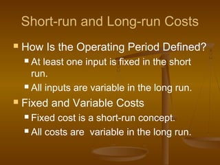
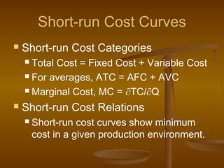
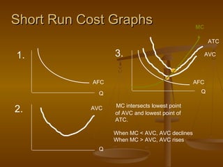
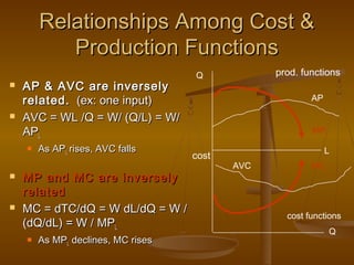
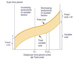
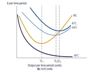
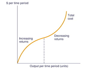
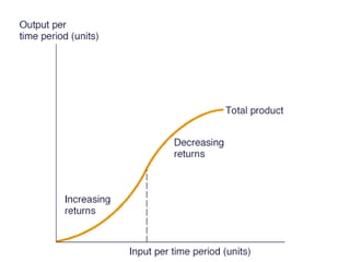
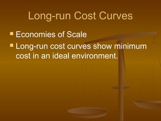
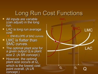
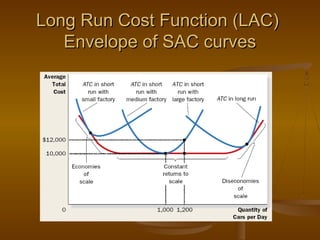
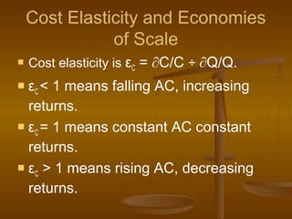
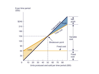
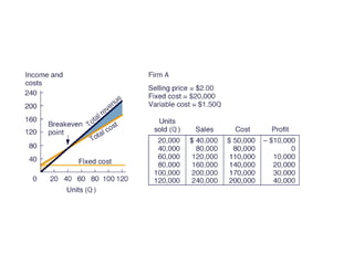
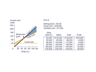
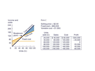
``
Cost Analysis andCost Analysis and
EstimationEstimation
What Makes Cost Analysis
Difficult?
 Link Between Accounting and Economic
Valuations
 Accounting and economic costs often differ.
 Historical Versus Current Costs
 Historical cost is the actual cash outlay.
 Current cost is the present cost of previously
acquired items.
 Replacement Cost
 Cost of replacing productive capacity using
current technology.
Opportunity Cost
 Opportunity Cost Concept
 Opportunity cost is foregone value.
 Reflects second-best use.
 Explicit and Implicit Costs
 Explicit costs are cash expenses.
 Implicit costs are noncash expenses.
Incremental and Sunk Costs in
Decision Analysis
 Incremental Cost
 Incremental cost is the change in cost tied to
a managerial decision.
 Incremental cost can involve multiple units of
output.
 Marginal cost involves a single unit of output.
 Sunk Cost
 Irreversible expenses incurred previously.
 Sunk costs are irrelevant to present decisions.
Short-run and Long-run Costs
 How Is the Operating Period Defined?
 At least one input is fixed in the short
run.
 All inputs are variable in the long run.
 Fixed and Variable Costs
 Fixed cost is a short-run concept.
 All costs are variable in the long run.
Short-run Cost Curves
 Short-run Cost Categories
 Total Cost = Fixed Cost + Variable Cost
 For averages, ATC = AFC + AVC
 Marginal Cost, MC = ∂TC/∂Q
 Short-run Cost Relations
 Short-run cost curves show minimum
cost in a given production environment.
Short Run Cost GraphsShort Run Cost Graphs
AFC
Q
Q
1.
2. AVC
3.
Q
AFC
AVC
ATC
MC
MC intersects lowest point
of AVC and lowest point of
ATC.
When MC < AVC, AVC declines
When MC > AVC, AVC rises
Relationships Among Cost &Relationships Among Cost &
Production FunctionsProduction Functions
 AP & AVC are inverselyAP & AVC are inversely
related.related. (ex: one input)(ex: one input)
 AVC = WL /Q = W/ (Q/L) = W/AVC = WL /Q = W/ (Q/L) = W/
APAPLL
 As APAs APLL rises, AVC fallsrises, AVC falls
 MP and MC are inverselyMP and MC are inversely
relatedrelated
 MC = dTC/dQ = W dL/dQ = W /MC = dTC/dQ = W dL/dQ = W /
(dQ/dL) = W / MP(dQ/dL) = W / MPLL
 As MPAs MPLL declines, MC risesdeclines, MC rises
prod. functions
cost functions
MPL
L
MC
AP
AVC
Q
Q
cost
Long-run Cost Curves
 Economies of Scale
 Long-run cost curves show minimum
cost in an ideal environment.
Long Run Cost FunctionsLong Run Cost Functions
 All inputs are variableAll inputs are variable
(can adjust) in the long(can adjust) in the long
run.run.
 LAC is long run averageLAC is long run average
costcost
 ENVELOPE of SAC curvesENVELOPE of SAC curves
 LMC is flatter thanLMC is flatter than
SMC curves.SMC curves.
 The optimal plant size forThe optimal plant size for
a given output Qa given output Q22 is plantis plant
size 2. (A SR concept.)size 2. (A SR concept.)
 However, the optimalHowever, the optimal
plant size occurs at Qplant size occurs at Q33,,
which is the lowest costwhich is the lowest cost
point overall. (A LRpoint overall. (A LR
concept.)concept.)
Q
LAC
LMCSAC2
SMC2
Q2 Q3
Long Run Cost Function (LAC)Long Run Cost Function (LAC)
Envelope of SAC curvesEnvelope of SAC curves
Cost Elasticity and Economies
of Scale
 Cost elasticity is εC = ∂C/C ÷ ∂Q/Q.
 εC < 1 means falling AC, increasing
returns.
 εC = 1 means constant AC constant
returns.
 εC > 1 means rising AC, decreasing
returns.
Long-run Average Costs
Economists think that the LAC is U-Economists think that the LAC is U-
shapedshaped
 Downward section due to:Downward section due to:
 Product-level economiesProduct-level economies which include specializationwhich include specialization
and learning curve effects.and learning curve effects.
 Plant-level economiesPlant-level economies, such as economies in, such as economies in
overhead, required reserves, investment, oroverhead, required reserves, investment, or
interactions among products (economies of scope).interactions among products (economies of scope).
 Firm-level economiesFirm-level economies which are economies inwhich are economies in
distribution and transportation of a geographicallydistribution and transportation of a geographically
dispersed firm, or economies in marketing, salesdispersed firm, or economies in marketing, sales
promotion, or R&D of multi-product firms.promotion, or R&D of multi-product firms.
CRS region
MES
Max ES
DRS
LAC
 Flat section of the LACFlat section of the LAC
 Displays constant returns to scaleDisplays constant returns to scale
 The minimum efficient scale (MES) is the smallestThe minimum efficient scale (MES) is the smallest
scale at which minimum per unit costs arescale at which minimum per unit costs are
attained.attained.
 Upward rising section of LAC is due to:Upward rising section of LAC is due to:
 Diseconomies of scale. These includeDiseconomies of scale. These include
transportation costs, imperfections in the labortransportation costs, imperfections in the labor
market, and problems of coordination and controlmarket, and problems of coordination and control
by management.by management.
 The maximum efficient scale (Max ES) is theThe maximum efficient scale (Max ES) is the
largest scale before which unit costs begin to rise.largest scale before which unit costs begin to rise.
 Modern business management offers techniquesModern business management offers techniques
to avoid diseconomies of scale through profitto avoid diseconomies of scale through profit
centers, transfer pricing, and tying incentives tocenters, transfer pricing, and tying incentives to
Economies of Scope
 Economies of Scope Concept
 Scope economies are cost advantages that
stem from producing multiple outputs.
 Big scope economies explain the popularity of
multi-product firms.
 Without scope economies, firms specialize.
 Exploiting Scope Economies
 Scope economics often shape competitive
strategy for new products.
Cost-volume-profit Analysis
 Cost-volume-profit Charts
 Cost-volume-profit analysis shows effects of
varying scale.
 Breakeven analysis shows zero profit points
of cost coverage.
Cost function
Cost function
Cost function
Cost function

Cost function

  • 1.
    `` Cost Analysis andCostAnalysis and EstimationEstimation
  • 2.
    What Makes CostAnalysis Difficult?  Link Between Accounting and Economic Valuations  Accounting and economic costs often differ.  Historical Versus Current Costs  Historical cost is the actual cash outlay.  Current cost is the present cost of previously acquired items.  Replacement Cost  Cost of replacing productive capacity using current technology.
  • 3.
    Opportunity Cost  OpportunityCost Concept  Opportunity cost is foregone value.  Reflects second-best use.  Explicit and Implicit Costs  Explicit costs are cash expenses.  Implicit costs are noncash expenses.
  • 4.
    Incremental and SunkCosts in Decision Analysis  Incremental Cost  Incremental cost is the change in cost tied to a managerial decision.  Incremental cost can involve multiple units of output.  Marginal cost involves a single unit of output.  Sunk Cost  Irreversible expenses incurred previously.  Sunk costs are irrelevant to present decisions.
  • 5.
    Short-run and Long-runCosts  How Is the Operating Period Defined?  At least one input is fixed in the short run.  All inputs are variable in the long run.  Fixed and Variable Costs  Fixed cost is a short-run concept.  All costs are variable in the long run.
  • 6.
    Short-run Cost Curves Short-run Cost Categories  Total Cost = Fixed Cost + Variable Cost  For averages, ATC = AFC + AVC  Marginal Cost, MC = ∂TC/∂Q  Short-run Cost Relations  Short-run cost curves show minimum cost in a given production environment.
  • 7.
    Short Run CostGraphsShort Run Cost Graphs AFC Q Q 1. 2. AVC 3. Q AFC AVC ATC MC MC intersects lowest point of AVC and lowest point of ATC. When MC < AVC, AVC declines When MC > AVC, AVC rises
  • 8.
    Relationships Among Cost&Relationships Among Cost & Production FunctionsProduction Functions  AP & AVC are inverselyAP & AVC are inversely related.related. (ex: one input)(ex: one input)  AVC = WL /Q = W/ (Q/L) = W/AVC = WL /Q = W/ (Q/L) = W/ APAPLL  As APAs APLL rises, AVC fallsrises, AVC falls  MP and MC are inverselyMP and MC are inversely relatedrelated  MC = dTC/dQ = W dL/dQ = W /MC = dTC/dQ = W dL/dQ = W / (dQ/dL) = W / MP(dQ/dL) = W / MPLL  As MPAs MPLL declines, MC risesdeclines, MC rises prod. functions cost functions MPL L MC AP AVC Q Q cost
  • 13.
    Long-run Cost Curves Economies of Scale  Long-run cost curves show minimum cost in an ideal environment.
  • 14.
    Long Run CostFunctionsLong Run Cost Functions  All inputs are variableAll inputs are variable (can adjust) in the long(can adjust) in the long run.run.  LAC is long run averageLAC is long run average costcost  ENVELOPE of SAC curvesENVELOPE of SAC curves  LMC is flatter thanLMC is flatter than SMC curves.SMC curves.  The optimal plant size forThe optimal plant size for a given output Qa given output Q22 is plantis plant size 2. (A SR concept.)size 2. (A SR concept.)  However, the optimalHowever, the optimal plant size occurs at Qplant size occurs at Q33,, which is the lowest costwhich is the lowest cost point overall. (A LRpoint overall. (A LR concept.)concept.) Q LAC LMCSAC2 SMC2 Q2 Q3
  • 15.
    Long Run CostFunction (LAC)Long Run Cost Function (LAC) Envelope of SAC curvesEnvelope of SAC curves
  • 16.
    Cost Elasticity andEconomies of Scale  Cost elasticity is εC = ∂C/C ÷ ∂Q/Q.  εC < 1 means falling AC, increasing returns.  εC = 1 means constant AC constant returns.  εC > 1 means rising AC, decreasing returns.
  • 17.
  • 18.
    Economists think thatthe LAC is U-Economists think that the LAC is U- shapedshaped  Downward section due to:Downward section due to:  Product-level economiesProduct-level economies which include specializationwhich include specialization and learning curve effects.and learning curve effects.  Plant-level economiesPlant-level economies, such as economies in, such as economies in overhead, required reserves, investment, oroverhead, required reserves, investment, or interactions among products (economies of scope).interactions among products (economies of scope).  Firm-level economiesFirm-level economies which are economies inwhich are economies in distribution and transportation of a geographicallydistribution and transportation of a geographically dispersed firm, or economies in marketing, salesdispersed firm, or economies in marketing, sales promotion, or R&D of multi-product firms.promotion, or R&D of multi-product firms.
  • 19.
    CRS region MES Max ES DRS LAC Flat section of the LACFlat section of the LAC  Displays constant returns to scaleDisplays constant returns to scale  The minimum efficient scale (MES) is the smallestThe minimum efficient scale (MES) is the smallest scale at which minimum per unit costs arescale at which minimum per unit costs are attained.attained.  Upward rising section of LAC is due to:Upward rising section of LAC is due to:  Diseconomies of scale. These includeDiseconomies of scale. These include transportation costs, imperfections in the labortransportation costs, imperfections in the labor market, and problems of coordination and controlmarket, and problems of coordination and control by management.by management.  The maximum efficient scale (Max ES) is theThe maximum efficient scale (Max ES) is the largest scale before which unit costs begin to rise.largest scale before which unit costs begin to rise.  Modern business management offers techniquesModern business management offers techniques to avoid diseconomies of scale through profitto avoid diseconomies of scale through profit centers, transfer pricing, and tying incentives tocenters, transfer pricing, and tying incentives to
  • 20.
    Economies of Scope Economies of Scope Concept  Scope economies are cost advantages that stem from producing multiple outputs.  Big scope economies explain the popularity of multi-product firms.  Without scope economies, firms specialize.  Exploiting Scope Economies  Scope economics often shape competitive strategy for new products.
  • 21.
    Cost-volume-profit Analysis  Cost-volume-profitCharts  Cost-volume-profit analysis shows effects of varying scale.  Breakeven analysis shows zero profit points of cost coverage.