
Recommended
More Related Content
Similar to Correlation Between SAT and GWA
Similar to Correlation Between SAT and GWA (20)
Recently uploaded
Recently uploaded (20)
Correlation Between SAT and GWA
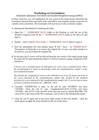
- 1. Workshop on Correlation: Scholastic Admission Test (SAT) and Graded Weighted Average (GWA) Seminar – Workshop 1 In these exercises, you will standardize the raw scores of the target group; determine the correlation between their percentile ranks and GWA; and compare groups using the sex variable in the correlation. The Scatterplot will also be use in the correlation output. A. Opening the Spreadsheets Containing the Data. 1. Open the WORKSHOP_DATA folder at the Desktop or with the use of the Windows Explorer look for the WORKSHOP_DATA folder in the Drive D: and open it. 2. Double – click TARGET.XLS in the WORKSHOP_DATA folder to open it. 3. Save the spreadsheet file with another name File – Save – As “EXER05.XLS”. The purpose of doing this is to reserve the original file. In case, you make mistakes in the process, you can reopen the original file. B. In this part, the Z–scores will be derived from the raw scores of the target group using the mean (42.91) and standard deviation (12.264) of normative group composed of 961 examinees. Z–Scores are a transformation of individual raw scores into a standard form, where the transformation is based on knowledge about the standardization sample’s mean and standard deviation. The formula for computing Z–scores is the individual raw score (X) minus the mean of the scores obtained by the standardization sample (M), divided by the standard deviation of scores obtained by the standardization sample (sd). Z–scores have a mean of 0 and a standard deviation of 1. (BROCK, 2012). 4. Currently, ‘EXER05.XLS is open. At the cell J2, type “ZCORES” and press <ENTER>. Click the cell J3, type ‘=standardize(E3,42.91,12.264)’ and press <ENTER>. The cell E3 is the location of the first raw score at column RSCORE. The value 42.91 is the mean of the 961 examinees, and 12.264 is the Standard Deviation. 5. Click the cell J3 again and at the lower right corner of this cell, double – click the small square to apply the same formula to the rest of the items.
- 2. Workshop on Correlation: Scholastic Admission Test (SAT) and Graded Weighted Average (GWA) Seminar – Workshop 2 C. Exporting the Data from EXERO5.XLS to IBM SPSS 6. Click File Save As. The File – Save As Dialog Appears. In the ‘Save as Type’ section, select ‘Text (Tab delimited)’. Filename is still ‘EXER05’. Then click Save. 7. Click the Yes button.
- 3. Workshop on Correlation: Scholastic Admission Test (SAT) and Graded Weighted Average (GWA) Seminar – Workshop 3 8. Click File Exit and then click No button. 9. Open IBM SPSS 16.0 or different version. If the opening window appears, just click the Cancel button. 10.Click File Read Text Data.
- 4. Workshop on Correlation: Scholastic Admission Test (SAT) and Graded Weighted Average (GWA) Seminar – Workshop 4 11. The Open Data dialog box appears. Go the WORKSHOP_DATA folder and look for ‘EXER05.TXT’ and then click the Open button. 12.The Text Import Wizard appears. Click Next in ‘Step 1 of 6’ window. 13.Click ‘Yes’ to answer the question “Are the variable names included at the top of your file?. Then, click next.
- 5. Workshop on Correlation: Scholastic Admission Test (SAT) and Graded Weighted Average (GWA) Seminar – Workshop 5 14. Click Next on ‘Step 3 of 6’ to ‘Step 5 of 6’. Finally, click ‘Finish’ on ‘Step 6 of 6’. 15. Save your file as ‘EXER05.SAV. NOTE: You can skip sections D to F and go directly to section G. Section G focuses on the correlation between RSCORE and GWA. D. In this part, you will compute the Percentile Ranks of the target group based on their Z–scores. 16.Click TRANSFORM > COMPUTE. Type “PRCTLRANK” in the TARGET VARIABLE box. Select “CDF & NONCENTRAL CDF” from the FUNCTION GROUP box. Select “CDF.NORMAL” function from the FUNCTIONS AND SPECIAL VARIABLES box. Click the up arrow , select “ZSCORES” from the variable box and click the right arrow to replace the first “?” inside the function CDF.NORMAL(?,?,?). Type “0” for the second “?” represents the mean and type “1” for the third “?” representing standard deviation. Click OK. The resulting screen is shown. CDF.NORMAL(ZSCORES,0,1)
- 6. Workshop on Correlation: Scholastic Admission Test (SAT) and Graded Weighted Average (GWA) Seminar – Workshop 6 17.In creating the column PRANK100, click TRANSFORM > COMPUTE VARIABLE. Type “PRANK100” in the TARGET VARIABLE box. Select “PRCNTLRANK” from the variables box and click the right arrow , to move it to NUMERIC EXPRESSION box. Complete the numeric expression by type “* 100”. The purpose of this expression is to convert the percentile ranks to the nearest ones. Then click OK. PRCNTLRANK * 100
- 7. Workshop on Correlation: Scholastic Admission Test (SAT) and Graded Weighted Average (GWA) Seminar – Workshop 7 E. In this part, you will be creating another column similar to stanine but have five scales only. The table below will be used. FIVE SCALES VERBAL DESCRIPTION RANGES OF PERCENTILE RANKS PERCENTAGES STANINE SCALE 5 Superior (4%) 96 and above 4% 9 89 – 95 7% 8 4 Above Average (19%) 77 – 88 12% 7 60 – 76 17% 6 40 – 59 20% 5 3 Average (54%) 23 – 39 17% 4 11 – 22 12% 3 2 Below Average (19%) 4 – 10 7% 2 1 Low (4%) Below 4 4% 1 18.In the menu, click TRANSFORM > XY RECODE INTO DIFFERENT VARIABLES. Select PRANK100 from the variable box at the left and move it into the INPUT VARIABLE OUTPUT VARIABLE box by clicking the right arrow . Type “FSCALE” into the NAME box and LABEL box at the OUTPUT VARIABLE section. Then click the CHANGE button.
- 8. Workshop on Correlation: Scholastic Admission Test (SAT) and Graded Weighted Average (GWA) Seminar – Workshop 8 Then click the OLD AND NEW VALUES button. Perform the following steps in entering the different ranges of percentile ranks for each scale: Type 0 in the RANGE box and 3.9 in the THROUGH box. Type 1 in the VALUE under the NEW VALUE section and then click the ADD button in the OLD NEW section. Type 4 in the RANGE box and 22.4 in the THROUGH box. Type 2 in the VALUE under the NEW VALUE section and then click the ADD button in the OLD NEW section. Type 22.5 in the RANGE box and 76.4 in the THROUGH box. Type 3 in the VALUE under the NEW VALUE section and then click the ADD button in the OLD NEW section. Type 76.5 in the RANGE box and 95.4 in the THROUGH box. Type 4 in the VALUE under the NEW VALUE section and then click the ADD button in the OLD NEW section. Type 95.5 in the RANGE box and 100 in the THROUGH box. Type 5 in the VALUE under the NEW VALUE section and then click the ADD button in the OLD NEW section. The resulting screen is shown. Click the CONTINUE button. Then OK. The column FSCALE is added.
- 9. Workshop on Correlation: Scholastic Admission Test (SAT) and Graded Weighted Average (GWA) Seminar – Workshop 9 F. In this part, you will be creating the histogram of the column FSCALE. 19.At the menu, click GRAPHS > LEGACY DIALOGS > HISTOGRAM. Select FSCALE from the variables box, click the right arrow. Click DISPLAY NORMAL CURVE. Click OK. The resulting histogram is shown. Next, save your file. G. Correlation Between RSCORES and GWA using Pearson Product Moment Correlation (PPMC). Correlation refers to any of a broad class of statistical relationships involving between two random variables or two sets of data (Correlation and Dependence, 2012). One way to express correlation is by the use of Pearson Product Moment Correlation coefficient. The Pearson Product – Moment Correlation Coefficient (r), or correlation coefficient for short is a measure of the degree of linear relationship between two variables, usually labeled X and Y. The correlation coefficient may take on any value between plus and minus one. (Stockburger, 1996)
- 10. Workshop on Correlation: Scholastic Admission Test (SAT) and Graded Weighted Average (GWA) Seminar – Workshop 10 20. At the ANALYZE menu, click CORRELATE > BIVARIATE. Select RSCORE and GRADE and move to the VARIABLES box using the right–arrow . By default, PEARSON, TWO–TAILED, and FLAG SIGNIFICANT CORRELATIONS are already selected. Click OPTIONS button, check MEANS AND STANDARD DEVIATIONS. Then click CONTINUE. Next, click OK.
- 11. Workshop on Correlation: Scholastic Admission Test (SAT) and Graded Weighted Average (GWA) Seminar – Workshop 11 21. Save the viewer file as ‘EXER0501”. These are the information you can see in the output. The correlation coefficient between RSCORE and GRADE is 0.260, which is a weak correlation.. The p–value is found in the row of Sig (2–tailed). The p–value is 0.009 which is lesser than the alpha value of 0.05, and marginal to 0.01. This means that there is a significant relationship between SEX and RSCORE. H. In this part, you will be using the Scatterplot graph. 22.At the GRAPHS menu, click LEGACY DIALOGS > SCATTER/DOT…. and then select SIMPLE SCATTER and click the DEFINE button.
- 12. Workshop on Correlation: Scholastic Admission Test (SAT) and Graded Weighted Average (GWA) Seminar – Workshop 12 The DEFINE SIMPLE SCATTER PLOT dialog. Move the RSCORE variable to X–AXIS, and GRADE variable to Y–AXIS and then click OK. The resulting graph is shown. To add a FIT LINE through the scattered dots, double–click on the graph to display the CHART EDITOR. At the CHART EDITOR click the ADD FIT LINE AT TOTAL icon. By the time you click the ADD FIT LINE AT TOTAL icon, its PROPERTIES dialog will appear. Simply click the CLOSE button of the PROPERTIES dialog, then click FILE > CLOSE the CHART EDITOR to close. The resulting graph is shown.
- 13. Workshop on Correlation: Scholastic Admission Test (SAT) and Graded Weighted Average (GWA) Seminar – Workshop 13 The Line of Best Fit or Fit Line is inclined upward to the right. Finally, save your file. I. In this part, you will perform the Subgroup Correlations by Sex 23.You need to get SPSS to calculate the correlation between RSCORE and GWA separately for males represented as 1 and females represented as 2. The easiest way to do this is to split our data file by sex. In the main menu, select DATA > SPLIT FILE. Select ORGANIZE OUTPUT BY GROUPS and GROUPS BASED ON SEX. This means that any analyses you specify will be run separately for males and females. Then, click Ok. Notice that the order of the data files has been changed. It is now sorted by SEX, with males at the top of the file.
- 14. Workshop on Correlation: Scholastic Admission Test (SAT) and Graded Weighted Average (GWA) Seminar – Workshop 14 Now, select ANALYZE > CORRELATION > BIVARIATE. The same variables and options you selected last time are still in the dialog box. Click OPTIONS button, check MEANS AND STANDARD DEVIATIONS. Then click CONTINUE. Then, click OK. Take a moment to check to see for you. The output follow broken down by males (1) and females (2). Display results for Males:
- 15. Workshop on Correlation: Scholastic Admission Test (SAT) and Graded Weighted Average (GWA) Seminar – Workshop 15 Display results for Females: J. Scatterplots of Data by Subgroups In this part, you will create a more complicated scatterplot that illustrates the pattern of correlation for males and females on one graph. 24.First, you need to turn off SPLIT FILE. Select DATA > SPLIT FILE from the main menu. Then select ANALYZE ALL CASES, do not compare groups and click OK. Now, you can proceed. The SPLIT FILE is turn off.
- 16. Workshop on Correlation: Scholastic Admission Test (SAT) and Graded Weighted Average (GWA) Seminar – Workshop 16 25.Select GRAPHS > LEGACY > SCATTER. Then, select SIMPLE and click DEFINE. Select GRADE as the Y Axis and RSCORE as the X Axis. Then, select SEX for SET MARKERS BY. This means SPSS will distinguish the males dots from the female dots on the graph. Then, click OK. To distinguish clearly the dots from the males and females, you will edit the graph. Double click the graph to activate the CHART EDITOR.
- 17. Workshop on Correlation: Scholastic Admission Test (SAT) and Graded Weighted Average (GWA) Seminar – Workshop 17 Then double click on one of the female (2) dots. SPSS will highlight all the female dots. Then click the MARKER menu. Select the CIRCLE under MARKER TYPE and chose a Fill color. Then click APPLY. Then CLOSE. You can do the same procedure for the male (1) dots by double clicking on the male dot as a start. Choose a different color for the male. 26. You would like to alter our graph to include the line of best fit for the male and female groups. Under ELEMENTS, select FIT LINE at SUBGROUPS. Then select LINEAR and click APPLY and CLOSE. Lastly, in the CHART EDITOR, click FILE > CLOSE.
- 18. Workshop on Correlation: Scholastic Admission Test (SAT) and Graded Weighted Average (GWA) Seminar – Workshop 18 The resulting graph follows. Finally, save your files. References: Brock, S. E. Descriptive Statistics and Psychological Testing. California State University, Sacramento. Retrieved April 05, 2012. Correlation. In http://www.uvm.edu. Retrieved August 21, 2012, from http://www.uvm.edu/~dhowell/fundamentals7/SPSSManual/SPSSLongerManual /SPSSChapter5.pdf Correlation and Dependence (2012, March 16). In http://www.wikipedia.org. Retrieved August 21, 2012, from http://www.wikipedia/correlation_and_ dependence.html Cohen, R. J., & Swerdlik, M. E. (2005). Psychological Testing and Assessment: An Introduction to Tests and Measurement. (6th Edition.) McGraw–Hill. Stockburger, D. W. (1996). Introductory Statistics: Concepts, Models, and Applications. Atomic Dog Publishing. Missouri State University Zucker, S. (2003, December). Fundamentals of Standardized Testing. Retrieved April 06, 2012 from http://www.hemweb.com.
- 19. Workshop on Correlation: Scholastic Admission Test (SAT) and Graded Weighted Average (GWA) Seminar – Workshop 19 Contents of TARGET.XLS:
- 20. Workshop on Correlation: Scholastic Admission Test (SAT) and Graded Weighted Average (GWA) Seminar – Workshop 20
- 21. Workshop on Correlation: Scholastic Admission Test (SAT) and Graded Weighted Average (GWA) Seminar – Workshop 21
- 22. Workshop on Correlation: Scholastic Admission Test (SAT) and Graded Weighted Average (GWA) Seminar – Workshop 22