Content adaptive single image interpolation based Super Resolution of compressed images

International Journal of Electrical and Computer Engineering (IJECE)
Vol. 10, No. 3, June 2020, pp. 3014~3021
ISSN: 2088-8708, DOI: 10.11591/ijece.v10i3.pp3014-3021  3014
Journal homepage: http://ijece.iaescore.com/index.php/IJECE
Content adaptive single image interpolation based Super
Resolution of compressed images
Amanjot Singh1
, Jagroop Singh2
1
I. K. Gujral Punjab Technical University, India
1
SEEE, Lovely Professional University, India
2
Department of Electronics and Communication Engineering, DAVIET, India
Article Info ABSTRACT
Article history:
Received Apr 7, 2019
Revised Jan 4, 2020
Accepted Jan 10, 2020
Image Super resolution is used to upscale the low resolution Images. It is also
known as image upscaling. This paper focuses on upscaling of compressed
images with interpolation based Single Image Super Resolution technique.
A content adaptive interpolation method of image upscaling has been
proposed. This interpolation based scheme is useful for single image based
Super Resolution methods. The presented method works on horizontal,
vertical and diagonal directions of an image separately and it is adaptive to
the local content of an image. This method relies only on a single image and
uses the content of the original image only; therefore, the proposed method is
more practical and realistic. The simulation results have been compared to
other standard methods with the help of various performance matrices like
PSNR, MSE, MSSIM etc. which indicates the preeminence of the proposed
method.
Keywords:
High resolution
Image upscaling
Interpolation
Low resolution
Super Resolution
Copyright © 2020 Institute of Advanced Engineering and Science.
All rights reserved.
Corresponding Author:
Amanjot Singh,
I. K. Gujral Punjab Technical University,
Punjab, India.
Email: er.ajotsingh@gmail.com
1. INTRODUCTION
In today's time, multimedia content in the digital data is growing day by day, which leads to a very
practical challenge of storage and transmission of multimedia content. It is due to the limitations of various
resources in different applications. In order to solve the issue specifically, multimedia data is transmitted in the
downscaled and compressed form under some standards. However, when it comes to the user side, that
multimedia data containing images or videos might have lost its original quality due to downscaling and
compression. As far as images are concerned, they mostly exist in downscaled and compressed formats.
In addition to images, videos are also compressed in various formats. Furthermore, many time due to heavy
quality reduction the original size of images get reduced. Hence, there is always a need of upscaling method
for reproducing a good quality image or to increase the number of pixels of images. Upscaling method should
not only upgrade the visual appearance but also make the images useful for other applications.
Super Resolution (SR) is one the most famous solution for these types of issues which can be achieved in
multiple ways. There are many advance ways to implement the SR, but one of the best practical solutions to
implement the Super Resolution of images is interpolation, which is less time consuming as well as requires
less computation. In many standard practical applications already interpolation is working for upscaling or
resizing of images. Interpolation based SR is having many applications, such as medical imaging, HDTV,
computer vision, satellite imaging and video surveillance etc.
Interpolation based approach is one of the fastest methods for image Super Resolution. Interpolation
based zooming schemes are frequently used in the real-time when working with small images. Nearest
neighbour (NN), bilinear and bicubic are the mostly used interpolation techniques [1-3]. These techniques are

Int J Elec & Comp Eng ISSN: 2088-8708 
Content adaptive single image interpolation based Super Resolution of compressed images (Amanjot Singh)
3015
non-adaptive, so these are computationally efficient but suffer from the problems of aliasing, blurring;
therefore, there are chances that these techniques could be improved further [4, 5]. However, this class of
methods could be used practically in many applications due to their simplicity. There are several edge directed
and non-linear interpolation schemes which have been developed to minimize the problems faced by
non-adaptive interpolation schemes [6-10]. In these techniques, re-sampling information is determined
according to the geometrical regularities that again requires the time and increases complexity. Some adaptive
interpolation based approaches [11-15] are present in literature but they are also having high computational
work or may be limited to a particular type of images. Higher order derivative and other high computation
based interpolation methods have also been presented in the literature [16-22]. However, the methods related
to the interpolation could be improved further and an effort has been done in this work to implement
the interpolation for upscaling or super resolution of images. Consequently, there is always a tradeoff between
system complexity and image quality. In this paper, a content adaptive SR method based upon interpolation
has been proposed. In this work proposed method works differently for the horizontal, vertical and diagonal
directions. Further, in section 2, interpolation based up-scaling has been explained, section 3 presents the proposed
method, section 4 deals with results analysis and in the last section 5, the conclusion has been drawn.
2. INTERPOLATION BASED IMAGE UP-SCALING
Image interpolation focuses on creating the high resolution image from its lower resolution version of
the image. Image interpolation is basically a method of artificially increasing the number of pixels in an area
inside an image. It is one of the methods which are usually present in the image processing applications like
facial reconstructions, image Super-Resolution, and multiple image descriptions etc. Image interpolation is
also one of the traditional methods used in the Super Resolution. Conventional systems include the bilinear
and bicubic interpolations which are having good real time computational simplicity. These require very
limited arithmetic operations [23-25]. Video interpolation or inter frame interpolation can also be achieved by
these methods. Other, Conventional systems based on polynomials interpolation methods are also present in
literature as discussed in previous section. Interpolation based approach is one of the fastest methods for image
Super Resolution. However, it produces the artifacts like blurriness, aliasing effects, nonrealistic edges etc.,
so there is still scope of improvement in these methods. Interpolation based SR schemes are more frequently
used when working with a single image only. Nearest Neighbor (NN), bilinear and bicubic are the ordinarily
used interpolation techniques. In order to execute the interpolation, there are also other various techniques as
described in the previous section. However, the three fundamental categories i.e. nearest neighbour, bilinear
and bi-cubic interpolation are used as the base of image interpolation. All these techniques have their own basic
defined procedures. Nearest neighbour interpolation is a replicating type of interpolation. It is a very basic
method and has its advantage of having very less computation. Moreover, because of the lesser computation,
its time consumption is also very less. Therefore, it is a good candidate for faster processing for image
upscaling. It is just repeating the values of neighbours, so it is not changing any original data. Bilinear
interpolation is another technique used for interpolation which is based on the average of pixels. It calculates
the average in the horizontal and vertical directions. It is computationally heavier than the nearest neighbour;
however, results are expected to be more favourable. Bicubic interpolation is based on a weighted average of
16 closest neighbours. It is more complex than other methods. However, in certain cases, it gives better results
than other techniques. It consumes more time compared to previous methods.
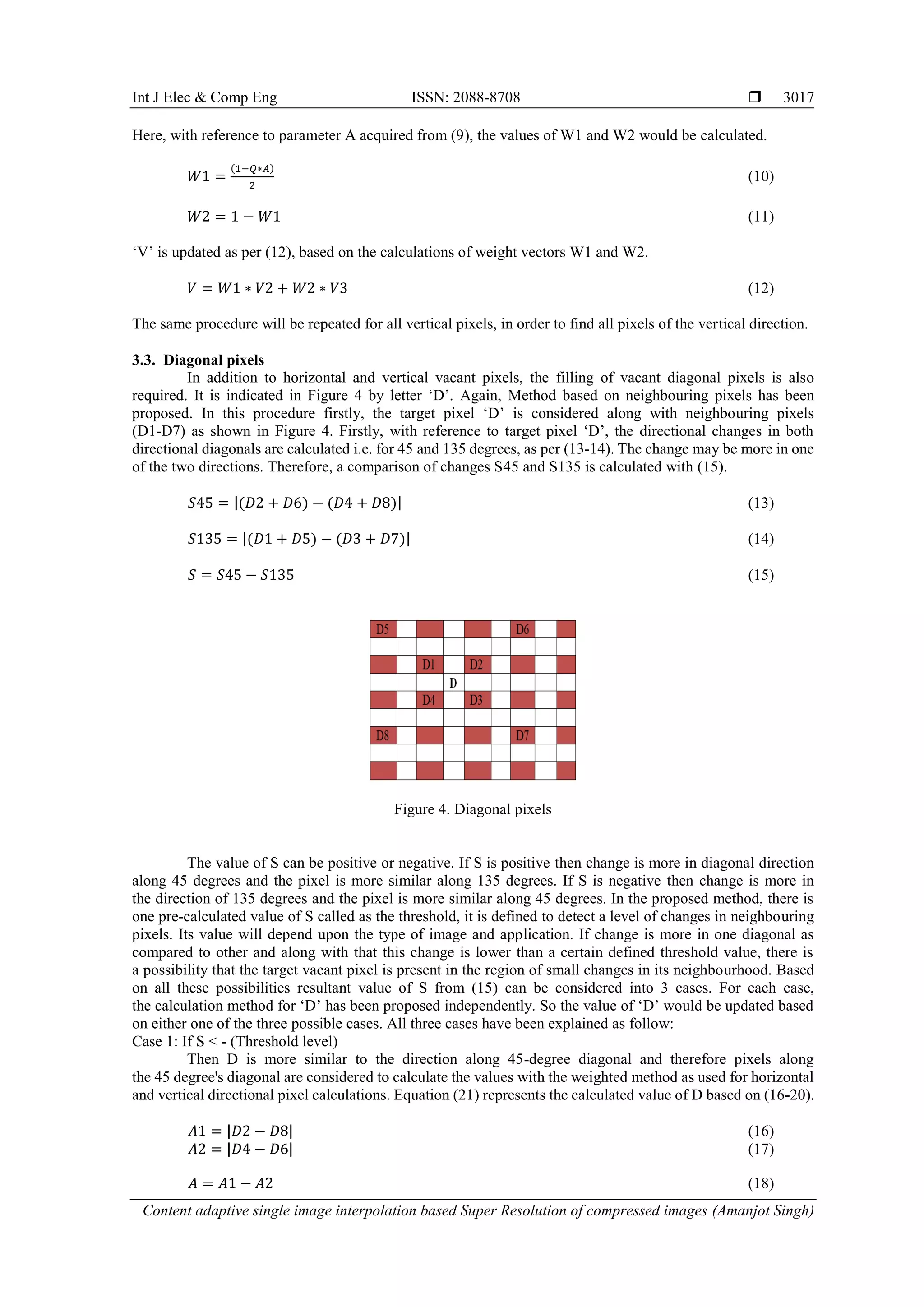
3. PROPOSED CONTENT ADAPTIVE INTERPOLATION METHOD
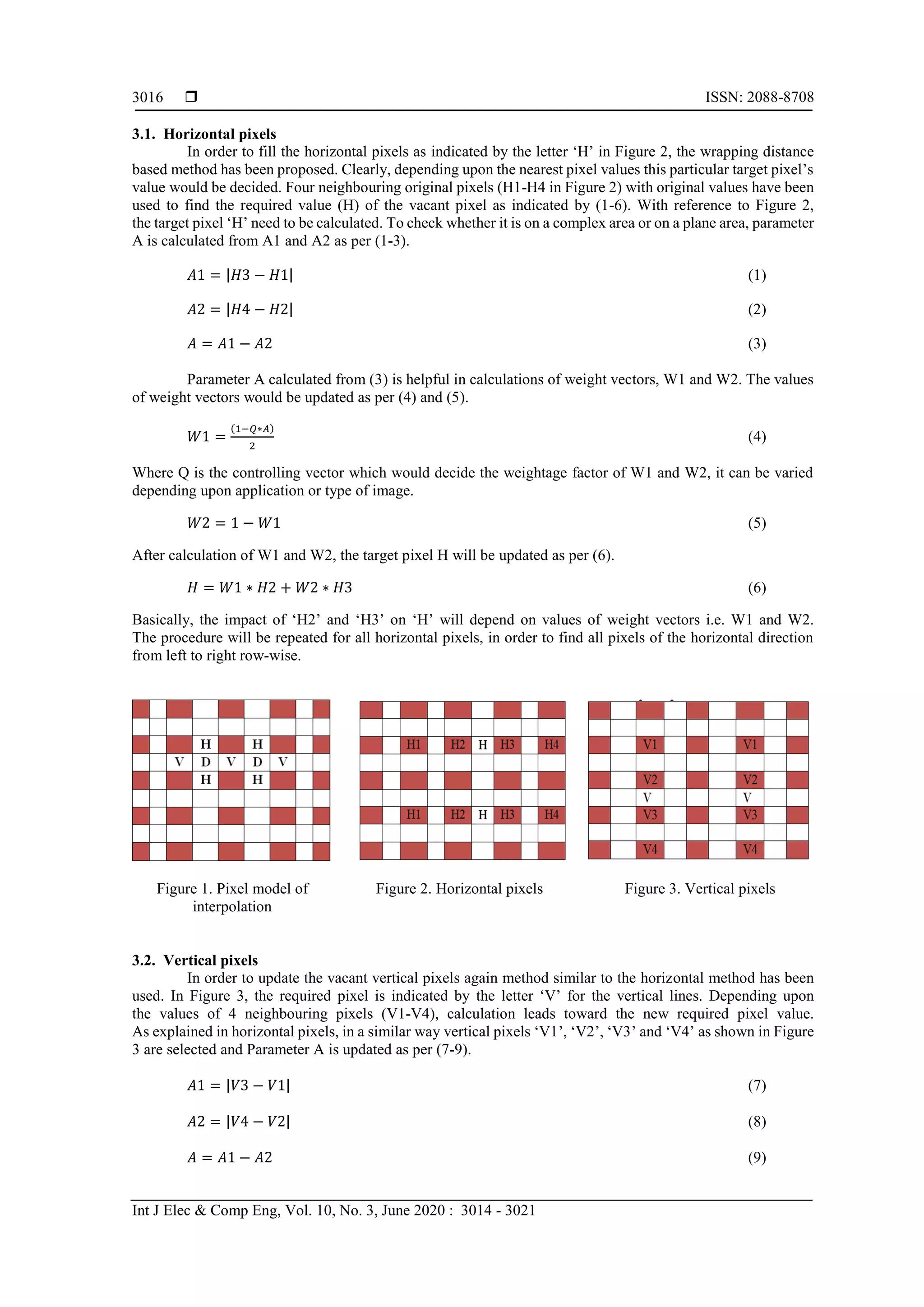
In the proposed method, the image of size ‘m’ x ‘n’ has been converted to ‘2m’ x ‘2n’ pixel image.
In order to upscale the image pixels are considered on a image pixel model of size ‘2m’ x ‘2n’ as shown in
Figure 1. In this model, the shaded blocks in Figure 1 represent the original pixels of an image and unshaded
blocks represent the vacant pixels which are required to be interpolated. In the process of filling vacant pixels,
the actual pixel values of the original image have been considered. In this method, the given image pixels have
been considered into three sorts; one is for filling of horizontal vacant pixels, second is for filling of vertical
vacant pixels and third is for filling of diagonally middle pixels as shown in Figure 1 with letters ‘H’, ‘V’ and
‘D’ respectively. Depending upon the particular direction of change, pixels are updated as per the methods
explained further with their respective sorts. Moreover, for all pixels, at least 4 original neighbouring pixels
are considered and then the value of the vacant pixel is calculated. In these methods, quantitative variations of
original pixel intensities have been considered based upon that proper value of vacant pixel would be assigned.
There are various possibilities of content which can exist in the images; there could be a complex region having
edges or other uniform smooth regions. Therefore, vacant pixel calculations will depend upon the content of
the region. The vacant pixel calculations involved in the three sorts are explained further.

 ISSN: 2088-8708
Int J Elec & Comp Eng, Vol. 10, No. 3, June 2020 : 3014 - 3021
3016
3.1. Horizontal pixels
In order to fill the horizontal pixels as indicated by the letter ‘H’ in Figure 2, the wrapping distance
based method has been proposed. Clearly, depending upon the nearest pixel values this particular target pixel’s
value would be decided. Four neighbouring original pixels (H1-H4 in Figure 2) with original values have been
used to find the required value (H) of the vacant pixel as indicated by (1-6). With reference to Figure 2,
the target pixel ‘H’ need to be calculated. To check whether it is on a complex area or on a plane area, parameter
A is calculated from A1 and A2 as per (1-3).
𝐴1 = |𝐻3 − 𝐻1| (1)
𝐴2 = |𝐻4 − 𝐻2| (2)
𝐴 = 𝐴1 − 𝐴2 (3)
Parameter A calculated from (3) is helpful in calculations of weight vectors, W1 and W2. The values
of weight vectors would be updated as per (4) and (5).
𝑊1 =
(1−𝑄∗𝐴)
2
(4)
Where Q is the controlling vector which would decide the weightage factor of W1 and W2, it can be varied
depending upon application or type of image.
𝑊2 = 1 − 𝑊1 (5)
After calculation of W1 and W2, the target pixel H will be updated as per (6).
𝐻 = 𝑊1 ∗ 𝐻2 + 𝑊2 ∗ 𝐻3 (6)
Basically, the impact of ‘H2’ and ‘H3’ on ‘H’ will depend on values of weight vectors i.e. W1 and W2.
The procedure will be repeated for all horizontal pixels, in order to find all pixels of the horizontal direction
from left to right row-wise.
Figure 1. Pixel model of
interpolation
Figure 2. Horizontal pixels Figure 3. Vertical pixels
3.2. Vertical pixels
In order to update the vacant vertical pixels again method similar to the horizontal method has been
used. In Figure 3, the required pixel is indicated by the letter ‘V’ for the vertical lines. Depending upon
the values of 4 neighbouring pixels (V1-V4), calculation leads toward the new required pixel value.
As explained in horizontal pixels, in a similar way vertical pixels ‘V1’, ‘V2’, ‘V3’ and ‘V4’ as shown in Figure
3 are selected and Parameter A is updated as per (7-9).
𝐴1 = |𝑉3 − 𝑉1| (7)
𝐴2 = |𝑉4 − 𝑉2| (8)
𝐴 = 𝐴1 − 𝐴2 (9)

3017
Here, with reference to parameter A acquired from (9), the values of W1 and W2 would be calculated.
𝑊1 =
(1−𝑄∗𝐴)
2
(10)
𝑊2 = 1 − 𝑊1 (11)
‘V’ is updated as per (12), based on the calculations of weight vectors W1 and W2.
𝑉 = 𝑊1 ∗ 𝑉2 + 𝑊2 ∗ 𝑉3 (12)
The same procedure will be repeated for all vertical pixels, in order to find all pixels of the vertical direction.
3.3. Diagonal pixels
In addition to horizontal and vertical vacant pixels, the filling of vacant diagonal pixels is also
required. It is indicated in Figure 4 by letter ‘D’. Again, Method based on neighbouring pixels has been
proposed. In this procedure firstly, the target pixel ‘D’ is considered along with neighbouring pixels
(D1-D7) as shown in Figure 4. Firstly, with reference to target pixel ‘D’, the directional changes in both
directional diagonals are calculated i.e. for 45 and 135 degrees, as per (13-14). The change may be more in one
of the two directions. Therefore, a comparison of changes S45 and S135 is calculated with (15).
𝑆45 = |(𝐷2 + 𝐷6) − (𝐷4 + 𝐷8)| (13)
𝑆135 = |(𝐷1 + 𝐷5) − (𝐷3 + 𝐷7)| (14)
𝑆 = 𝑆45 − 𝑆135 (15)
Figure 4. Diagonal pixels
The value of S can be positive or negative. If S is positive then change is more in diagonal direction
along 45 degrees and the pixel is more similar along 135 degrees. If S is negative then change is more in
the direction of 135 degrees and the pixel is more similar along 45 degrees. In the proposed method, there is
one pre-calculated value of S called as the threshold, it is defined to detect a level of changes in neighbouring
pixels. Its value will depend upon the type of image and application. If change is more in one diagonal as
compared to other and along with that this change is lower than a certain defined threshold value, there is
a possibility that the target vacant pixel is present in the region of small changes in its neighbourhood. Based
on all these possibilities resultant value of S from (15) can be considered into 3 cases. For each case,
the calculation method for ‘D’ has been proposed independently. So the value of ‘D’ would be updated based
on either one of the three possible cases. All three cases have been explained as follow:
Case 1: If S < - (Threshold level)
Then D is more similar to the direction along 45-degree diagonal and therefore pixels along
the 45 degree's diagonal are considered to calculate the values with the weighted method as used for horizontal
and vertical directional pixel calculations. Equation (21) represents the calculated value of D based on (16-20).
𝐴1 = |𝐷2 − 𝐷8| (16)
𝐴2 = |𝐷4 − 𝐷6| (17)
𝐴 = 𝐴1 − 𝐴2 (18)

 ISSN: 2088-8708
3018
𝑊1 =
(1−𝑄∗𝐴)
2
(19)
𝑊2 = 1 − 𝑊1 (20)
𝐷 = 𝑊1 ∗ 𝐷2 + 𝑊2 ∗ 𝐷4 (21)
Case 2: If S > + (Threshold level)
Then D is more similar to the direction of 135-degree diagonal and therefore, pixels along the 135
degree's diagonal are considered to calculate the values with the weighted method as used for horizontal and
vertical direction with (22-27).
𝐴1 = |𝐷3 − 𝐷5| (22)
𝐴2 = |𝐷7 − 𝐷1| (23)
𝐴 = 𝐴1 − 𝐴2 (24)
𝑊1 =
(1−𝑄∗𝐴)
2
(25)
𝑊2 = 1 − 𝑊1 (26)
𝐷 = 𝑊1 ∗ 𝐷1 + 𝑊2 ∗ 𝐷3 (27)
Case 3: Otherwise i.e. – (Threshold level) ≤ S ≤ (Threshold level)
If the value of S from (15) is lying between the negative thresholds to a positive threshold, then it is
taken as the third case. If the difference S in pixels is lying in this range, then it contains the finer details for
which again procedure is defined. In this case, a window of 4 x 4 pixels (D1-D16) is selected as shown in
Figure 5 and in this a particular window mean is calculated. Based upon that standard deviation is calculated
and thus it is detected that whether it is a soft edge or a fine area. The deviation limit L should be based on
the type of image and it should provide the best results at that value.
Figure 5. Pixel window of the original image
If the Standard deviation of the window (4 X 4) > (Deviation limit L), then it is a soft edge.
Therefore, minimum nearest pixels will be used to calculate the unknown diagonal pixel ‘D’. In order to update
the target pixel ‘D’, different pixels as shown in Figure 5 would be considered as per (28).
𝐷 =
𝐷1+𝐷2+𝐷3+𝐷4
4
(28)
Else, if the Standard deviation of the window (4 X 4) ≤ (Deviation limit L), It represents the area of some
smoother finer region and weight matrix is used to calculate the unknown pixels. The weight matrix is given
by (29) which is used to update pixels.
𝑊 = [
0.0127 0.0436 0.0436 0.0127
0.0436 0.1500 0.1500 0.0436
0.0436 0.1500 0.1500 0.0436
0.0127 0.0436 0.0436 0.0127
] (29)

3019
In this case, the target vacant pixel ‘D’ can be calculated as per (32) which involves the element wise
matrix multiplication of pixels (D1-D16) with weight matrix (Wrc) i.e. Wrc . Drc . Here, Drc represents the matrix
of original pixels (D1-D16) as shown in Figure 5.
𝑊𝑟𝑐 = [
𝑤11 ⋯ 𝑤1𝑛
⋮ ⋱ ⋮
𝑤 𝑛1 ⋯ 𝑤 𝑛𝑛
] (30)
𝐷𝑟𝑐 = [
𝐷11 ⋯ 𝐷1𝑛
⋮ ⋱ ⋮
𝐷 𝑛1 ⋯ 𝐷 𝑛𝑛
] (31)
The value n will be 4 in case of soft smooth area:
𝐷 = ∑ 𝑊𝑟𝑐. 𝐷𝑟𝑐
𝑛 𝑛
𝑟=1 𝑐=1 (32)
The procedure having 3 cases will be repeated for the all Diagonal ‘D’ vacant pixels in the complete
image and the values of all unknown target pixels would be calculated. In this way all the new pixels at ‘H’,
‘V’ and ‘D’ are calculated in three sorts, which are used for increasing the number of pixels or super-resolving
the required image. Clearly, above procedure can be repeated depending upon the level of Super Resolution
i.e. depending upon magnification factor.
4. RESULTS AND ANALYSIS
In order to compare the performance of method, an analysis has been performed further. In the analysis
part lossy compression has been considered which includes the standard compressions. Test images are taken
of size 256 x 256 pixels and have been converted to 512 x 512 pixels as a part of SR. All the test images are
compressed images with two standards i.e. the “JPEG”, “JPEG2000” and the level of compression or quality
of test images is related with the bit rate of the test image. It has been seen that the proposed method performs
better than other standard methods as shown in Figure 6.
Test image ‘Lena’ Nearest Bilinear Bicubic
Ref.[12] Ref.[13] Proposed Method
Figure 6. Comparison of Interpolation techniques for jpg compressed images for the upper right part
For the purpose of finding which particular algorithms give an improved result, it requires
the organized comparative system. Clearly, same test image database is required to be tested on image
interpolation methods. In order to evaluate the performance of the method well known quality metrics like
Peak signal-to-noise ratio (PSNR), Mean-square error (MSE) could be used. MSSIM is mean structural
similarity index, again a very useful index for qualitative comparisons [26]. Multiple images have been
considered, for which PSNR, MSE and MSSIM of the proposed method have been compared with Nearest
Neighbor, Bilinear, Bi-Cubic interpolation along with method given by Ref. [12] and Ref. [13] respectively.

 ISSN: 2088-8708
3020
Results have been shown in Tables 1 and 2, for JPEG and JPEG2000 based compressed images separately.
Under all these performance metrics the proposed method has performed better than the standard methods.
Table 1. Comparison of interpolation techniques for JPEG compressed images
Image Bit Rate Parameter Proposed Method Nearest Bilinear Bicubic Ref. [12] Ref. [13]
Lena.jpg 0.82 PSNR 35.13 29.63 31.53 31.53 34.36 34.02
MSE 19.91 70.73 45.69 45.73 23.80 25.74
MSSIM 0.920 0.864 0.894 0.897 0.913 0.910
Child.jpg 0.90 PSNR 34.64 29.49 31.50 31.49 33.97 33.76
MSE 22.31 73.07 45.97 46.08 26.02 27.32
MSSIM 0.935 0.875 0.908 0.912 0.926 0.924
Fruits.jpg 0.85 PSNR 32.24 27.40 29.20 29.17 31.53 30.92
MSE 38.80 118.17 78.02 78.71 45.68 52.50
MSSIM 0.901 0.842 0.872 0.873 0.893 0.887
Peppers.jpg 0.95 PSNR 32.81 28.56 30.2 30.23 32.39 32.10
MSE 34.02 90.47 60.91 61.65 37.49 40.02
MSSIM 0.844 0.788 0.821 0.820 0.838 0.836
Cameraman.jpg 0.78 PSNR 35.56 27.97 30.31 30.44 35.08 34.11
MSE 18.05 103.72 60.44 58.75 20.20 25.20
MSSIM 0.958 0.902 0.930 0.936 0.949 0.948
Table 2. Comparison of interpolation techniques for JPEG2000 compressed images
Image Bit Rate Parameter Proposed Method Nearest Bilinear Bicubic Ref. [12] Ref. [13]
Lena.jp2 0.3830 PSNR 34.71 29.32 31.23 31.13 34.06 33.77
MSE 22.01 76.00 49.04 50.10 25.51 27.30
MSSIM 0.908 0.854 0.882 0.884 0.902 0.899
Child.jp2 0.3843 PSNR 34.00 29.19 31.16 31.06 33.46 33.33
MSE 25.91 78.43 49.79 50.89 29.34 30.23
MSSIM 0.915 0.859 0.890 0.892 0.907 0.906
Fruits.jp2 0.3835 PSNR 31.73 27.23 28.96 28.90 31.12 30.60
MSE 43.62 123.16 82.71 83.74 50.28 56.65
MSSIM 0.877 0.827 0.851 0.852 0.870 0.865
Peppers.jp2 0.3827 PSNR 32.14 28.32 29.90 29.82 31.81 31.63
MSE 39.75 95.69 66.53 67.74 42.88 44.70
MSSIM 0.817 0.772 0.798 0.798 0.812 0.812
Cameraman.jp2 0.3836 PSNR 35.30 27.79 30.18 30.21 34.89 34.00
MSE 19.20 108.17 62.44 61.98 21.11 25.86
MSSIM 0.949 0.892 0.921 0.925 0.941 0.940
With reference to results, it is quite clear that as the compression standard changes, the performance
of up-scaling methods differs. In both the methods when the bit rate is low i.e. compression level is high, the
performance of each algorithm is low. However, as the bit rate increases performance of interpolation improves
further. It is due to the reason that as bits rate increases, compression ratio decreases, therefore the quality of
base image also increases. As both considered standards are lossy compression standards, there is always some
loss of data. If compression would be high then there will be an additional need of denoising or deblocking
method along with interpolation. However, the proposed method has performed better than
the other conventional methods. The proposed method is based on interpolation hence it cannot be compared
with other training based methods which require a training database and often consume more time as compared
to interpolation based methods. The proposed method is more practical and further performance can be
enhanced by including other noise removal methods to enhance the quality of the base image.
5. CONCLUSION
In this paper, the presented content adaptive method of image up-scaling is based on adaptive
interpolation. This method uses a single image frame and works as the post processing method of Super
Resolution for the compressed images. The proposed method relies on a content adaptation of interpolation
technique. In the paper, BDCT based “JPEG” and wavelet based “JPEG2000” standard compressed images
have been considered in the analysis. With reference to the simulations and analysis, it can be concluded that
the proposed method performs better than other conventional standard methods in terms of different quality
matrices. The proposed system stands good for real life systems which require faster image Super Resolution.
In the upcoming days, up-scaling of videos is also required where frame by frame interpolation could be useful
and the proposed method can be modified to interpolate video signals also.

3021
REFERENCES
[1] Hou. HS, Andrews HC, “Cubic splines for image interpolation and digital filtering,” IEEE Transaction Acoust. Speech
Signal Process, vol. 26, pp. 508–517, 1978.
[2] Unser M, Aldroubi A and Eden M, “Fast B-spline transforms for continuous image representation and interpolation,”
IEEE Trans. Pattern Anal. Mach. Intell., pp. 77–85, 1991.
[3] Acharya T., Tsai P., “Computational Foundations of Image Interpolation Algorithms,” ACM Ubiquity, vol. 8, 2007.
[4] Amanatiadis A., Andreadis I., “A survey on evaluation methods for image interpolation,” Meas. Sci. Technology, vol.
20(10), pp. 1-9, 2009.
[5] A. Singh, J. Singh, “Super Resolution Applications in Modern Digital Image Processing,” International Journal of
Computer Applications, vol. 150(2), Sep. 2016.
[6] Li X., Orchard MT., “New edge-directed interpolation,” IEEE Trans Image Process, vol. 10, pp. 1521–1527, 2001.
[7] Ju. Y., Lee YJ., “Nonlinear image upsampling method based on radial basis function interpolation,” IEEE Trans Image
Process, vol. 19, pp. 2682–2692, 2010.
[8] Z. Xiong, X. Sun, and F. Wu, “Robust web image/video super-resolution,” IEEE Trans. Image Process., vol. 19(8),
pp. 2017–2028, 2010.
[9] L. Zhang and X. Wu, “An edge-guided image interpolation algorithm via directional filtering and data fusion,” IEEE
Transactions on Image Processing, vol. 15(8), pp. 2226–2238, 2006.
[10] Q. Wang and R.K. Ward, “A new orientation-adaptive interpolation method,” IEEE Transactions on Image
Processing, vol. 16(4), pp. 889–900, 2007.
[11] Hwang JW., and Lee HS., “Adaptive image interpolation based on local gradient features,” IEEE Signal Process Lett.,
vol. 11, pp. 359–362, 2004.
[12] M. Sajjad, N. Ejaz, I. Mehmood and S.W. Baik, “Digital image super-resolution using adaptive interpolation based on
Gaussian function,” Multimedia Tools and Applications, vol.74(20), pp. 8961-8977, 2015.
[13] Sunil P.J., et al., “A Low Complex Context Adaptive Image Interpolation Algorithm for Real-Time Applications,” in
2012 IEEE International Instrumentation and Measurement Technology Conference Proceedings, 2012.
[14] Suresha D., Prakash HN., “Single picture Super Resolution of natural images using N-Neighbor Adaptive Bilinear
Interpolation and absolute asymmetry based wavelet hard thresholding,” 2016 2nd International Conference on
Applied and Theoretical Computing and Communication Technology (iCATccT), pp. 387–393, 2016.
[15] Sajjad M., Ejaz N., Baik SW., “Multi-kernel based adaptive interpolation for image super-resolution,” Multimedia
Tools Appl., vol. 72, pp. 2063–2085, 2014.
[16] Deyun Wei, “Image super-resolution reconstruction using the high-order derivative interpolation associated with
fractional filter functions,” IET Signal Processing, IET Journals & Magazines, vol. 10(9), pp. 1052–1061, 2016.
[17] Liu, C. M., and Luo, X. N., “Image enlargement via interpolatory subdivision,” IET Image Process., vol. 5,
pp. 567–571, 2011.
[18] J. S. Choi and M. Kim, “Super-interpolation with edge-orientation-based mapping kernels for low complex 2×
upscaling,” IEEE Trans. Image Process., vol. 25(1), pp. 469–483, 2016.
[19] Y. Zhang, Q. Fan, F. Bao, Y. Liu, and C. Zhang, “Single-Image Super-Resolution Based on Rational Fractal
Interpolation,” IEEE Trans. Image Process., vol. 27(8), pp. 3782–3797, 2018.
[20] Zhu S., Zeng B., Zeng L., Gabbouj M., “Image Interpolation Based on Non-local Geometric Similarities and
Directional Gradients,” IEEE Transactions on Multimedia, vol. 18(9), pp. 1707–1719, 2016.
[21] Kim H., Cha Y., Kim S., “Curvature interpolation method for image zooming,” IEEE Trans Image Process, vol. 20,
pp. 1895-1903, 2011.
[22] Shuyuan Zhu, et al., “Image Interpolation Based on Non-local Geometric Similarities and Directional Gradients,”
IEEE Transactions on Multimedia, vol. 18(9), pp. 1707–1719, 2016.
[23] Amir Nazren Abdul Rahim, “An Analysis of Interpolation Methods for Super Resolution Images,” 2015 IEEE Student
Conference Research and Development (SCOReD), Dec. 2015.
[24] A. Singh and J. Singh, “Image Upscaling and Denoising with Gaussian filter in Coloured Images -A Performance
Analysis,” International Journal of Engineering and Technology (IJET), vol. 9(3), 2017.
[25] V.D. Earshia, M. Sumathi, “A Comprehensive Study of 1D and 2D Image Interpolation Techniques,” International
Conference on Communications and Cyber Physical Engineering 2018 (ICCCE 2018), pp. 383-391, 2018.
[26] Z. Wang, A. C. Bovik, H. R. Sheikh, E. P. Simoncelli, “Image quality assessment: from error measurement to structural
similarity,” IEEE Trans.on Image Process., vol. 3(4), pp. 600-612, Apr. 2004.

Content adaptive single image interpolation based Super Resolution of compressed images

More Related Content

What's hot

Similar to Content adaptive single image interpolation based Super Resolution of compressed images

More from IJECEIAES

Recently uploaded

Content adaptive single image interpolation based Super Resolution of compressed images