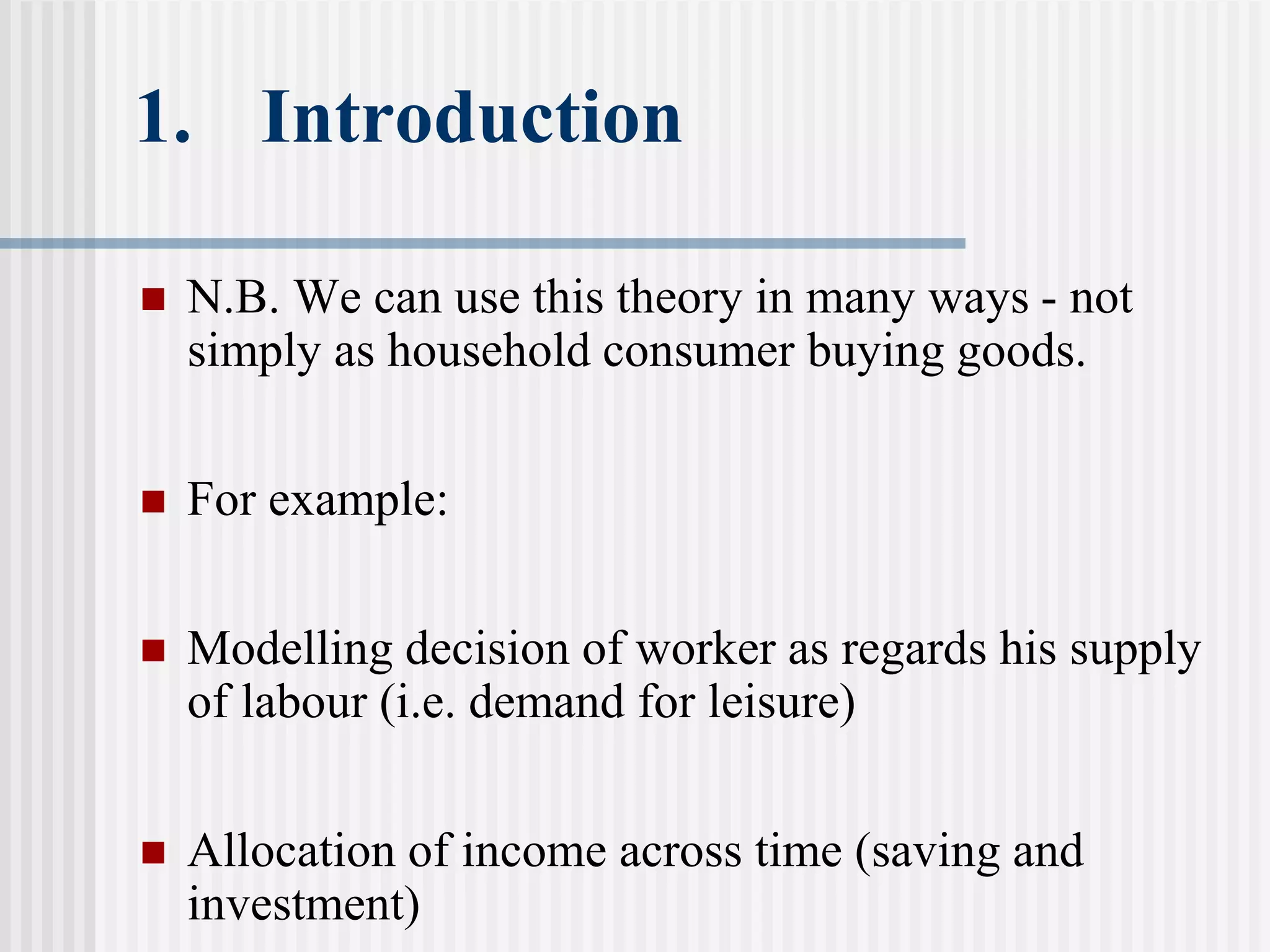
2. 1. Introduction
We have seen how demand curves may be used to
represent consumer behaviour.
But we said very little about the nature of the
demand curve; why it slopes down for example.
Now we go ‘behind’ the demand curve
i.e. we investigate how buyers reconcile what they
want with what they can get
3. 1. Introduction
N.B. We can use this theory in many ways - not
simply as household consumer buying goods.
For example:
Modelling decision of worker as regards his supply
of labour (i.e. demand for leisure)
Allocation of income across time (saving and
investment)
4. 2. Theory of Consumer Choice
Four elements:
(i) Consumer’s income
(ii) Prices of goods
(iii) Consumer’s tastes
(iv) Rational Maximisation
5. 3. The Budget Constraint
The first two elements define the budget constraint
The feasibility of the consumer’s desired
consumption bundle depends upon two factors:
(i) Income
(ii) Prices
Note: We assume, for the time being, that both are
exogenous (i.e. beyond consumer's control)
6. 3. The Budget Constraint
Example (N.B two goods)
Two goods - films and meals
Student grant = $50 per week (p.w.)
Price of meal = $5
Price of film = $10
7. 3. The Budget Constraint
Thus student can ‘consume’ maximum p.w. of 10
meals or 5 films by devoting all of his grant to the
consumption of only one of these goods.
Alternatively, he can consume some combination of
the two goods
For example, giving up one film a week (saving $10)
enables student to buy two additional meals (costing
$5 each)
.
11. 3. The Budget Constraint
The budget constraint defines the maximum
affordable quantity of one good available to the
consumer given the quantity of the other good that
is being consumed.
N.B. Trade-off!
Trade-off is represented slope of budget
constraint.
12. 3. The Budget Constraint
Intercepts
Determined by income divided by the appropriate
price of the good
Define maximum quantity of a particular good
available to an individual
Slope
Independent of income
Determined only by relative prices
• .
13. 3. The Budget Constraint
If consumer is devoting all income to films (qf =
$50/$10 = 5), then 1 meal can only be obtained by
sacrificing consumption of some films.
How many films must consumer give up?
pm = $5; thus to obtain that $5, the consumer must
give up 1/2 a film
14. 3. The Budget Constraint
The slope of the budget constraint in this
example is thus:
-
pm
pf
= -
$5
$10
= -
1
2
16. 3. The Budget Constraint
More generally:
Two goods (x,y), prices (px, py) and money income
(m)
m = pxx + pyy
Slope of budget constraint: - px/py
17. 3. The Budget Constraint
Proof:
m = px
x + py
y
Þ
py
y = m - px
x
Þ
y =
m
py
-
px
py
x
18. 3. The Budget Constraint
Thus:
Such that
y =
m
py
æ
è
ç
ö
ø
÷
a
-
px
py
æ
è
ç
ö
ø
÷
b
x
Þ
y = a - bx
Dy = -bDx = -
px
py
æ
è
ç
ö
ø
÷ Dx
20. 3. The Budget Constraint
Intuition:
If additional units of x costs px
Then their purchase requires a change in
consumption of y of –(px/py) (i.e. a sacrifice of y)
in order to maintain the budget constraint.
21. 3. The Budget Constraint
Economic Rate of Substitution (ERS)
Amount of y the consumer is obliged to
sacrifice for one extra unit of x
ERS = –(px/py)
Slope of budget line
22. 3. Budget Constraint
Taxes and Subsidies
Taxes can be imposed per unit (i.e. p + t) or ad
valorem [i.e. p(1+ t)]
Subsidies are ‘negative’ taxes
Rationing causes budget constraint to become
vertical or horizontal
24. y
0 xt m/px
Figure 5: Budget Constraint and Taxation
m/py
x
Slope = -(px/py)
Slope = -[(px+t)/py]
x
25. 4. Preferences
Consider now the consumer’s preferences; given
what consumer can do, what would he like to do?
Four assumptions:
(i) Completeness
(ii) Consistency
(iii) Non-satiation
(iv) Diminishing Marginal Rate of Substitution
26. 4. Preferences
Completeness
Consumers can rank alternative bundles according
to the satisfaction or utility they provide
Thus, given two bundles a and b, then ,
or
Preferences assumed only to be ordinal, not
cardinal; i.e. consumer simply has to be able to say
he prefers a to b, not to say by how much.
a ≻ b a ≻ b
a ≻ b
27. 4. Preferences
Consistency
Preferences are also assumed to be consistent
Thus if and , then we would infer that
We assume consumer is logically consistent
a ≻ b a ≻ c
a ≻ c
28. 4. Preferences
Non-satiation
Consumers assumed to always prefer more
‘goods’ to less.
We can accommodate economics ‘bads’ (e.g.
pollution) in this assumption by interpreting then
as ‘negative’ goods
We can illustrate the first three assumptions
graphically as follows
33. 4. Preferences
Marginal Rate of Substitution (MRS)
The quantity of y (i.e. the ‘vertical’ good) the consumer
must sacrifice to increase the quantity of x (i.e. ‘the
horizontal’ good) by one unit without changing total utility.
We generally assume (smooth) diminishing MRS
To hold utility constant, diminishing quantities of
one good must be sacrificed to obtain successive
equal increases in the quantity of the other good.
34. 4. Preferences
Diminishing MRS derives from underlying
assumption of diminishing marginal utility
Marginal utility of a good is defined as the change
in a consumer’s total utility from consuming the
good divided by the change in his consumption of
the good
Diminishing MRS assumes that the increase in
utility from consuming additional units of a good
is declining
35. 4. Preferences
Non-satiation implies downward sloping
indifference curves; increases in one good require
sacrifices in the other good to hold total utility
constant.
However, we can go further; diminishing MRS
implies that indifference curves are convex to
origin, becoming flatter as we move to the right.
Indeed, the MRS of x for y is simply the slope of
the indifference curve
40. 4. Preferences
Diminishing MRS implies consumers prefer
consumption bundles containing mixtures of
goods rather than extremes
For example, Bundle C = (5, 5) preferred to both
Bundle A = (2, 8) and Bundle B = (8, 2)
Diminishing MRS (i.e. diminishing marginal
utility)
48. 4. Preferences
Note:
(i) Any point on the indifference map must lay on
an indifference curve;
and
(ii) indifference curves cannot cross
Thus every point on the indifference map must lay
on one and only one indifference curve