Ml chalter

1. Unit- 3
Non Parameter methods
By: Ritu Agrawal
Assistant Professor,
CSE department, PIET, PU

2. •Parametric Vs. Non parametric estimation
•Non – parameter methods
•Application of non parametric estimation
•Tools for non parametric estimation
•Parzen-window method (PWM)
•Kernel Density Estimator
•Importance of PWM
Topics:

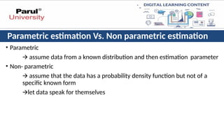
3. Parametric estimation Vs. Non parametric estimation
• Parametric
🡪 assume data from a known distribution and then estimation parameter
• Non- parametric
🡪 assume that the data has a probability density function but not of a
specific known form
🡪let data speak for themselves

4. Non-Parameter methods
• Non-parametric techniques for density estimation in pattern recognition refer
to methods that do not make explicit assumptions about the underlying
probability distribution of the data.
• Instead of assuming a specific functional form for the distribution, these
techniques aim to estimate the density directly from the data.
• Attempt to estimate the density directly from the data without making any
parametric assumptions about the underlying distribution

5. Nonparametric
Density Estimation

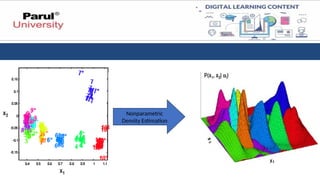
6. Application of Non-parametric techniques
• Non-parametric techniques and pattern recognition are closely connected,
as non-parametric methods provide valuable tools for analyzing and recognizing
patterns in data.
•Here's the correlation between non-parametric techniques and pattern recognition:
•Flexible Modeling
•Feature Extraction
•Dimensionality Reduction
•Density Estimation
•Data Visualization

7. Tools for Non-parametric techniques
•R
•Python
•Weka
•MATLAB
•SAS
•SPSS

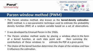
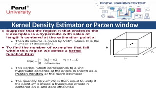
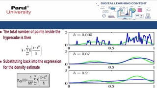
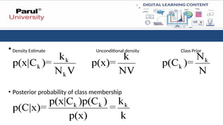
8. Parzen window method (PWM)
• The Parzen window method, also known as the kernel density estimation
(KDE) method, is a non-parametric technique used to estimate the probability
density function (PDF) of a random variable based on a set of observations.
• It was developed by Emanuel Parzen in the 1960s.
• The Parzen window method works by placing a window, often in the form
of a kernel function, at each data point and then summing the
contributions of these windows to estimate the PDF at a given point.
• The choice of the kernel function determines the shape of the window and how
it influences the estimation.

9. Steps involved in PWM
1. Data preparation
2. Choose a kernel function
3. Determine the window width
4. Place windows at each data point
5. Sum the contributions
6. Normalize the estimate

10. Kernel Density Estimator or Parzen window

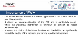
12. Importance of PWM
• The Parzen window method is a flexible approach that can handle data of
any dimensionality.
• It allows for smooth estimation of the PDF and is particularly useful
when the underlying distribution is unknown or difficult to model
parametrically.
• However, the choice of the kernel function and bandwidth can significantly
impact the quality of the estimate, and careful selection is important.

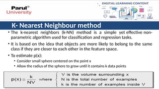
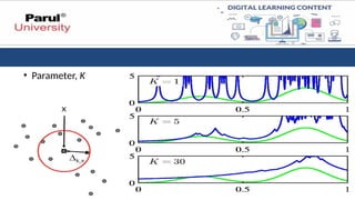
13. K- Nearest Neighbour method
• The k-nearest neighbors (k-NN) method is a simple yet effective non-
parametric algorithm used for classification and regression tasks.
• It is based on the idea that objects are more likely to belong to the same
class if they are closer to each other in the feature space.
• To estimate p(x):
• Consider small sphere centered on the point x
• Allow the radius of the sphere to grow until it contains k data points

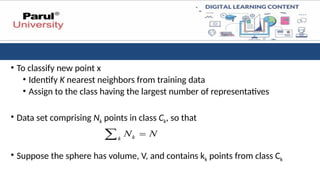
14. • To classify new point x
• Identify K nearest neighbors from training data
• Assign to the class having the largest number of representatives
• Data set comprising Nk points in class Ck, so that
• Suppose the sphere has volume, V, and contains kk points from class Ck

15. •Density Estimate Unconditional density Class Prior
• Posterior probability of class membership

16. • Parameter, K

17. Steps involved in KNN Method
• Data preparation
• Choose the value of k
• Calculate distances
• Select the k nearest neighbors
• Make predictions
• Evaluate performance.

18. Advantages of k-NN:
• Simple and Easy to Understand: k-NN is one of the simplest and most
intuitive machine learning algorithms.
• It requires minimal theoretical background to grasp the core idea.
• Effective for Certain Datasets: k-NN can be very effective for datasets
where the decision boundaries between classes are well-defined and the
data is evenly distributed.
• No Explicit Model Training: As a lazy learner, k-NN doesn't require upfront
model training, potentially saving computational time.

19. Disadvantages of k-NN:
• Curse of Dimensionality: As the number of features in the data increases, distance
metrics become less reliable, leading to performance degradation.
• Feature selection or dimensionality reduction techniques can help mitigate this issue.
• Computational Cost During Prediction: Predicting for new data points can be
computationally expensive, especially for large datasets, as k-NN needs to calculate
distances to all training data points.
• Sensitivity to k Value: The choice of the k value significantly impacts performance.
• A high k can lead to overfitting, while a low k might lead to underfitting.
• Experimentation is often needed to find the optimal value.

20. Non-metric methods for pattern classification
• Non-metric methods for pattern classification refer to approaches that
do not rely on explicit distance metrics or measures of similarity
between data points.
• These methods focus on other aspects of the data or employ alternative
techniques to perform pattern classification. Here are a few examples

21. Types of Non-metric methods
• Decision Trees
• Random Forest
• Support Vector Machines
• Neural Networks
• Naive Bayes
• Genetic Algorithms

22. Decision Trees
• Imagine a series of if-then-else questions that successively split your data into
smaller and purer subsets based on feature values.
• Decision trees operate on this foundation.
• They build a tree-like structure where each internal node represents a
question, each branch represents an answer, and the terminal nodes (leaves)
represent the predicted class labels.

23. Characteristic of decision tree
1.Training
• How do you construct one from training data?
• Entropy-based Methods
2. Strengths
• Easy to Understand
3. Weaknesses
• Overtraining

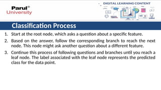
24. Classification Process
1. Start at the root node, which asks a question about a specific feature.
2. Based on the answer, follow the corresponding branch to reach the next
node. This node might ask another question about a different feature.
3. Continue this process of following questions and branches until you reach a
leaf node. The label associated with the leaf node represents the predicted
class for the data point.

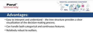
26. Advantages:
• Easy to interpret and understand – the tree structure provides a clear
visualization of the decision-making process.
• Can handle both categorical and continuous features.
• Relatively robust to outliers.

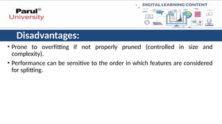
27. Disadvantages:
• Prone to overfitting if not properly pruned (controlled in size and
complexity).
• Performance can be sensitive to the order in which features are considered
for splitting.

28. Decision Tree: Structure
• At the core of a decision tree is a simple yet powerful concept.
• A series of if-then-else rules that are used to make a decision.
• The tree is composed of nodes, where each node represents a decision, and
branches, which represent the possible outcomes of that decision.
Hierarchical Decisions
• Decision trees work by making a series of hierarchical decisions, starting from the
root node and working down to the leaf nodes.
• At each internal node, the algorithm evaluates a feature of the input data and
selects the best split based on a chosen criterion, such as information gain or Gini
impurity.

29. Interpretability
• One of the key advantages of decision trees is their interpretability.
• The tree-like structure of the model makes it easy to understand the
reasoning behind the predictions, as each path from the root to a leaf node
represents a set of logical rules that can be easily communicated and
explained.

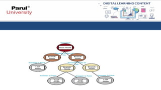
30. The Structure of a Decision Tree
• A Decision Tree consists of the following components:
1.Root Node: The topmost node, representing the entire dataset.
2.Decision Nodes: These nodes, also known as internal nodes, are
responsible for splitting the data into subsets based on input features.
3.Leaf Nodes: The terminal nodes, representing the predicted
outcomes or class labels.
4.Edges: The connections between nodes, illustrating the flow of data.

31. Constructing a Decision Tree

33. Splitting Nodes

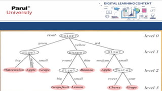
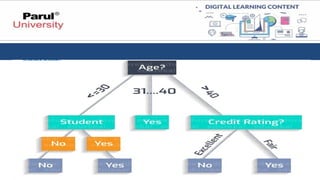
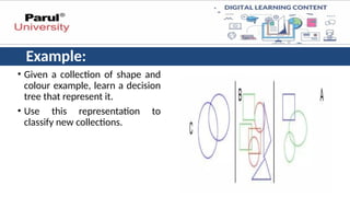
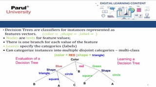
35. Example:
• Given a collection of shape and
colour example, learn a decision
tree that represent it.
• Use this representation to
classify new collections.

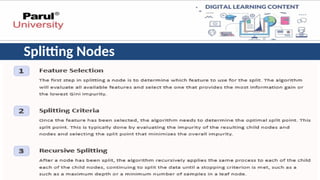
37. Choosing of the attributes
1: Information Gain
• One common criterion for selecting the best split is information gain, which
measures the reduction in entropy (or uncertainty) achieved by splitting the
data on a particular feature.
• The algorithm will choose the feature that provides the highest information
gain.
2: Gini Impurity
• Another popular splitting criterion is Gini impurity, which measures the
probability of a randomly chosen sample being misclassified if it was randomly
labeled according to the distribution of labels in the subset.

38. • The algorithm will choose the split that minimizes the Gini impurity of the
resulting child nodes.
3. Gain Ratio (Classification): This addresses a bias towards attributes with
many possible values by incorporating the information gain and the number of
splits needed for that attribute.
4. Chi-Square (Classification): This measures the statistical dependence
between an attribute and the target variable.
• A higher chi-square value suggests a stronger relationship, potentially leading
to a good split.

39. 5. Mean Squared Error (Regression): This measures the average squared
difference between the predicted and actual values after a split on an attribute.
• A lower mean squared error indicates a better split for regression tasks.
6. Other Criteria
• There are also other splitting criteria, such as variance reduction for regression
tasks and Chi-square for categorical variables.
• The choice of criterion will depend on the specific problem and the type of
data being used.

40. Stopping Criteria for Tree Growth

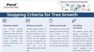
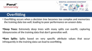
41. Overfitting
• Overfitting occurs when a decision tree becomes too complex and memorizes
the training data too well, leading to poor performance on unseen data.
•Deep Trees: Extremely deep trees with many splits can overfit, capturing
idiosyncrasies of the training data that don't generalize well.
•Rare Splits: Splits based on very specific attribute values that occur
infrequently in the training data can lead to overfitting.

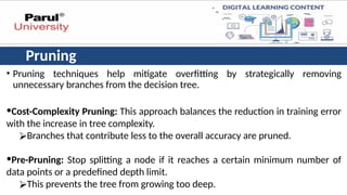
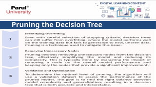
42. Pruning
• Pruning techniques help mitigate overfitting by strategically removing
unnecessary branches from the decision tree.
•Cost-Complexity Pruning: This approach balances the reduction in training error
with the increase in tree complexity.
⮚Branches that contribute less to the overall accuracy are pruned.
•Pre-Pruning: Stop splitting a node if it reaches a certain minimum number of
data points or a predefined depth limit.
⮚This prevents the tree from growing too deep.

43. • Post-Pruning: Build a full tree first and then selectively remove branches that
contribute little to accuracy on a validation set.
• By understanding attribute selection, overfitting, and pruning, you can
effectively build decision trees that are both accurate and generalizable.
• Remember, a well-crafted decision tree strikes a balance between capturing
the underlying patterns in your data and avoiding overfitting to the specifics of
the training data.

44. Pruning the Decision Tree