This master thesis focuses on both perturbative and non-perturbative methods of evaluating the Chern-Simons partition function on S3 with gauge group SU(2).
The first chapter introduces the relationship between Morse theory and supersymmetry, and shows its application in an instanton calculation. Chern-Simons theory is then identified as a crucial Morse function.
The first loop correction of Chern-Simons is calculated in the second chapter and is proportional to the Ray-Singer torsion of S3 with respect to a flat connection, up to a metric-dependent phase term. This phase term is shown to be independent of the metric up to a choice of framing.


![Introduction
The early motivation of this thesis is to understand recent developments in relations
between quantization and categorification[20, 21]. Also various naive interests of
the author in mysterious relations between number theory and physics turn out
to be much profound in modern understanding of non-Abelian extension of class
field theory, also called the geometric Langlands program. The electromagnetic
duality plays central role in physical construction of the program[22, 27, 18]. A
crucial ingredient in the field of study is the Chern-Simons theory which has a long
history in physics whilst it became more and more vital whence people started using
topological information to study theories of different dimensions. One can find a
more detailed motivation and discussion of results in the epilogue, and here we will
outline the contents of this thesis.
As one of the most celebrating theories of 20-th century, quantum field theory
suffers serious problem of divergences even disrespect the unsatisfactory underlining
mathematical formalism and the non-conventional physical reality that physicists
do not concern too much about since none of them seems solvable before the di-
vergences being removed. Therefore various solutions appeared since the theory
developed. It is interesting that if the extension is “appropriate”, one gets more
detail structures, and the problems remained do not worry people any more. How-
ever, divergences still exist until string theory and supersymmetry were introduced
to the game. The ultraviolet divergence in QFT is mainly caused by using of point
like particle, and when interactions are in short distances or even zero-distance in-
finity appears. By upgrading to higher dimensional particles, the problem resolved.
One interesting fact is that within a 2-dimensional world sheet, conformal sym-
metry translates a singular point to an infinite tube where different string states
exist, this is the operator-state correspondence, a short explanation in Appendix
G. If one looks at the Feynman diagram, this appropriate extension is just fatten
the one-dimensional world line to world sheet. The infrared divergence is gone by
adding supersymmetry. A satisfactory QFT is one major problem for theorists.
Another fundamental problem at central concern is the reconciliation of QFT
and gravity. It is the main driving force for many theorists. One seemingly profound
tool from Standard Model is gauge symmetry. With it one can gain pure geometric
information which is metric independent, thus we really have the desired general
covariance. CS captures such information, and among other intuitions Witten
1](https://image.slidesharecdn.com/96310c1d-2d9c-47cc-b2b3-bc64b84ba972-160405111747/75/Thesis-11-2048.jpg)
![2 Introduction
considered it as a QFT in [42]. The partition function of such theory is a generating
function of knots and it gives knot invariant, i.e. the Jones polynomial. Knots can
be physically represented by non-trivial Wilson loops in the theory, such that knot
invariant coincides with observables. On the other hand, the projection of a knot in
a plane has a lot of interesting properties related to physics. One simple example is
the Yang-Baxter equation from statistic physics and the third Reidemeister move.
Many applications to vertex model, quantum group, integrable system, etc tightly
related to CS[41, 43].
We will focus on topological information that can be extracted from supersym-
metry, therefore the first chapter introduces its relations to differential forms. Then
we continue to its beautiful relations to Morse theory which makes it possible to
calculate global invariants from local analytic functions. We carry out the instan-
ton calculation of supersymmetric non-sigma model to show how one can get the
topological data from the theory. Its realtions to CS is when one considers the
Morse function as CS. This is an example of non-relativistic three dimensional field
theory, the generalization to relativistic version is Donaldson theory of four mani-
folds which can be interpreted as a topological QFT. Along Floer homology many
interesting theories appear, unfortunately we will not talk about them but only
focus on CS first.
In the second chapter, we start with basic facts of CS. Then construct a QFT
with it. With standard Faddeev-Povov procedure we arrive the gauge fixed action
which has BRST symmetry, thus CS gives a topological theory. The first loop
correction carried out by the path integral is proportional to the Ray-Singer torsion,
which is topological invariant, up to a metric dependent phase term. Using APS
theorem one can see that the extra phase term is actually metric independent up to
a framing choice. Moreover, there is always a canonical 2-framing that the phase
term disappears. This essentially proves the theory is topological from perturbative
point of view.
In the last chapter, we use non-perturbative method to derive the exact result
of CS partition function on S3
and compare its asymptotic behavior to results
from previous chapter. This is the first example of AdS3/CFT2 correspondence.
To arrive the comparison, we briefly review the root lattice of simple Lie algebra
and extension to Kac-Moody algebra. Then derive the Kac-Weyl character formula
which can be used to construct the partition function. One can explicitly com-
pute the partition function by canonical quantization of CS on product manifolds,
geometric quantization or holomorphic quantization. Any of the cases shows the
partition function has modular invariance. However we choose an easier path. The
arriving of exact results is from simple arguments on surgeries of 3-manifolds which
can be considered as symmetry of modular forms. Finally the exact result gives
same classical behavior from perturbation point of view.
In the Epilogue we give a full motivation and discussions of the results for
a future reference. Hopefully this thesis can serve as a general introduction to
different aspects of CS and provide a overall guidance to proceed to modern theory
of gauge theory and low-dimensional topology.](https://image.slidesharecdn.com/96310c1d-2d9c-47cc-b2b3-bc64b84ba972-160405111747/75/Thesis-12-2048.jpg)

![4 Chapter 1. Supersymmetry and Morse theory
the same problem as classical model, the Higgs boson of it gives a divergent self-
energy correction and the scale limit is about 10(−17)
cm. Therefore supersymmetry
is introduced to double the degrees of freedom again and to cancel the divergence
of self-energy at scales beyond.
There are also many other beautiful theories to get beyond the Standard Model.
Since experiment scale has not reach TeV level yet, we cannot be so obsessed by
one’s beauty. However, we will focus on supersymmetry now as it’s natural existence
in the string theory and profound connections with geometry and topology.
1.2 Differential forms and supersymmetry
Supersymmetry is a symmetry between boson and fermion. Bosons are relatively
easier to imagine than fermions as anticommutativity is indeed unfamiliar to us,
just looking at ab = −ba. But how about the world of anticommute objects? They
may find us the peculiar one. This suggests a duality between these two different
perspectives. Can we find some rigorous mathematics to realize such duality?
Let M be a n-dimensional Riemannian manifold with metric γ, denote as (M, γ).
At each point p on M we can form tangent vectors ak
and their dual a†k
. Noticing
that a†k
can be regarded as operators on the exterior algebra at p, a†k
↔ dxk
∧.
With the Hodge star ∗ which maps Ωq
(M) → Ωn−q
(M), it follows that ak
are
operators with operation being interior multiplication, ak
↔ (−1)nq+n+1
∗ dxk
∗.
What we have done is nothing but separating the operations of exterior derivative
and its dual, see later Eq.(1.2). Most importantly, they obey anticommutation
relations
{ai
, aj
} = 0, {a†i
, a†j
} = 0, {ai
, a†j
} = γij
. (1.1)
These are desired fermionic relations we want. To involve bosons, recall the bosonic
momentum operators pk ↔ −i∂k. With these identifications, we can rewrite the
exterior derivative d and the co-differential d†
as
d = ia†k
pk, d†
= −iak
pk. (1.2)
Therefore we have commutation relations
[d, xk
] = a†k
, [d†
, xk
] = −ak
, (1.3)
and anticommutation relations
{d, a†j
} = 0, {d, aj
} = iγjk
pk, {d†
, a†j
} = −iγjk
pk, {d†
, aj
} = 0. (1.4)
From these relations, we can regard d and d†
as generators of exchanges between
fermionic operators ai
, a†i
and bosonic operators pi. They form a Z2 graded algebra.](https://image.slidesharecdn.com/96310c1d-2d9c-47cc-b2b3-bc64b84ba972-160405111747/75/Thesis-14-2048.jpg)
![1.2. Differential forms and supersymmetry 5
We can now define supercharges Qi, generators of suppersymmetry, as linear
combinations of d and d†
to be
Q1 = d + d†
, Q2 = i(d − d†
). (1.5)
The fact that d2
= d†2
= 0 implies {Q1, Q2} = 0 and Q2
1 = Q2
2 = {d, d†
}, which is
the Laplace-Beltrami operator ∆. If we can consider ∆ as the Hamiltonian operator
H, then we have the simplest supersymmetric quantum mechanics. The Lorentz
invariance indicates that the momentum operator P is zero in our case, that is to
say we are dealing with P = 0 subspace H0 of the total Hilbert space H .
Accordingly, we see that supersymmetry is of beauty with language of differen-
tial forms. Such elegant connection between physics and mathematics is introduced
by Witten in early 80s[38]. The motivation of Witten might be the deep connection
of supersymmetry and topology. Let us keep looking at some physical reasoning
again before going any further.
The first question about supersymmetry is that we cannot see it in nature, at
present scale limit. We have to know how to determine its presence in one the-
ory. Like other symmetries, supersymmetry must commute with the Hamiltonian
operator
[Qi, H] = 0, i = 1, . . . , N, (1.6)
where N is the number of supercharges. However, there are huge differences between
spontaneous breaking of supersymmetry than other internal symmetries. Since
H = Q2
i , any supersymmetric state |0 , which is a state annihilated by the Qi,
must has zero-energy and it is the true vacuum state. Therefore only if there is no
such a state, supersymmetry is spontaneously broken and the ground state will have
positive energy. For ordinary internal symmetries, the criteria for spontaneously
broken of symmetry is independent of the energy of ground state, e.g. the Mexican
hat potential.
Moreover, if supersymmetry is not broken, we can define an operator to dis-
tinguish bosonic and fermionic states. Recall supersymmetry is a Z2 graded al-
gebra, we can decompose the Hilbert space H0 into a direct sum two subspaces,
H0 = H +
0 ⊕ H −
0 , where H +
0 for bosonic states and H −
0 for fermionic states.
Then we can define (−1)F
as (−1)F
|b = |b for |b ∈ H +
0 , and (−1)F
|f = −|f
for |f ∈ H −
0 . Consequently, we have a basic condition must be satisfied by each
Qi
(−1)F
Qi + Qi(−1)F
= 0. (1.7)
A crucial observation by Witten[37] recognizes the trace of (−1)F
, the Witten
index, as a topological invariant. Let us assume there is only one supercharge Q.
Since supersymmetry is not broken, any state of non-zero energy has a super partner](https://image.slidesharecdn.com/96310c1d-2d9c-47cc-b2b3-bc64b84ba972-160405111747/75/Thesis-15-2048.jpg)

![1.3. Morse theory 7
This connection between physics and topology is so beautiful that there must
be profound reasons behind it. However, before unveil it, we still can do more
about the supersymmetric ground states. Whether nE=0
B and nE=0
F are invariants
themselves? If so, one simple constrain is needed, that is nE=0
B + nE=0
F must be a
invariant too. Let us see how this is possible. Consider now the theory is with two
supercharges Q1 and Q2, define a linear combination of them as
Q± =
1
2
(Q1 ± iQ2). (1.12)
It is readily to see the superalgebra
Q2
+ = Q2
− = 0, Q+Q− + Q−Q+ = H. (1.13)
We have recovered the exterior algebra introduced earlier, check Eq.(1.4). Q± are
exactly the exterior derivative d and the co-differential d†
. We see that the su-
persymmetric ground states, E = 0, are exactly the non-trivial elements of the
cohomology H•
(M, d). However, equivalent cohomologies are classified by homo-
topy class of the manifold.
Let us consider an one to one map U between supersymmetric states of different
systems, that is |˜b = U−1
|b . This is same as defining new operators
˜Q+ = U−1
Q+U,
˜Q− = UQ−U−1
,
˜H = ˜Q+
˜Q− + ˜Q−
˜Q+.
(1.14)
Consequently, for any state |Ω annihilated by Q+ or Q− there is a state |˜Ω
annihilated by ˜Q+ or ˜Q−. Furthermore, if U is unitary, U†
= U−1
, this corresponds
to a change of basis in Hilbert space and the two systems are the same. If it is not
unitary, the two systems are different whilst the number of zero-energy states are
same. Therefore changes of parameters that can be brought by conjugation will
not affect nE=0
B + nE=0
F and the numbers can be invariants independently.
By using these ideas Witten found that Tr(−1)F
of supersymmetric non-linear
sigma model is a topological invariant which equals to the Euler characteristic of
manifold M,
Tr(−1)F
= χ(M). (1.15)
This might probably be the reason Witten discovered the relation of supersymmetry
and Morse theory[38].
1.3 Morse theory
Morse theory enables us to study the topology of manifold M by analyse differen-
tiable functions on it. We will first give a brief introduction to Morse theory and
then see its connection with supersymmetry.](https://image.slidesharecdn.com/96310c1d-2d9c-47cc-b2b3-bc64b84ba972-160405111747/75/Thesis-17-2048.jpg)

![1.4. Instanton and Witten complex 9
1.4 Instanton and Witten complex
Recall the definition of supercharges by linear combination of d and d†
, Eq.(1.5),
we can generalize it by defining
dt = e−ht
deht
, d†
t = eht
d†
e−ht
, (1.17)
where h is the Morse function. Since d2
t = d†2
t = 0, we define
Q1t = dt + d†
t , Q2t = i(dt − d†
t ), Ht = dtd†
t + d†
t dt (1.18)
and the superalgebra is still hold for any t. The ground states will not change by
this conjugation as we argued before. That is, if we denote the Betti number as
bq(t), it is independent of t and equals to bq of M.
To write Ht in detail, we first note that
dt = e−ht
deht
= d + ta†i
∂ih
d†
t = eht
d†
e−ht
= d†
+ tai
∂ih,
(1.19)
and for a q-form ω
d(ai
∂ihω) = a†j
∂j(ai
∂ih)ω − ai
∂ihdω
d†
(a†j
∂jhω) = ai
∂ih(a†j
∂jhω) − a†j
∂jhd†
ω.
(1.20)
Therefore, we obtain
Ht = dd†
+ d†
d + t2
(dh)2
+
i,j
t
D2
h
DφiDφj
[a†i
, aj
], (1.21)
where D is the covariant derivative that Dih = ∂ih and ∂j(ai
Dih) = ai
DjDih with
DjDih = (∂j∂i − Γk
ji∂k)h, and (dh)2
= γij
∂ih∂jh is the square of the gradient of
h. Notice that we are working on Riemannian manifold (M, γ) introduced earlier.
Now we can see how Morse theory is related with supersymmetry. For large
t limit, the potential energy V (φ) = t2
(dh)2
becomes very large except near each
critical point, at which dh = 0. Therefore minimals of eigenvalues of Ht are localized
near the critical points and can be calculated by expanding about them. Near each
critical point Pq, the coordinates φi are Euclidean, and if we set φi = 0 to be Pq
then the metric tensor γ is Euclidean up to terms of order φ2
. Thus the Morse
function is approximated as h(φi) = h(0)+ 1
2 λiφ2
i +O(φ3
) for some λi. We have
Ht being approximated as
Ht =
i
(−
∂2
∂φ2
i
+ t2
λ2
i φ2
i + tλi[a†i
, ai
]). (1.22)
The corrections to this formula are determined by higher order terms of φ, but for
ground states they will not enter and thus reasonable to study ground states with
it.](https://image.slidesharecdn.com/96310c1d-2d9c-47cc-b2b3-bc64b84ba972-160405111747/75/Thesis-19-2048.jpg)
![10 Chapter 1. Supersymmetry and Morse theory
Let us denote
Hi = −
∂2
∂φ2
i
+ t2
λ2
i φ2
i , Ji = [a†i
, ai
]. (1.23)
It is readily to see that Hi and Jj mutually commute and can be simultaneously
diagonalized. Moreover, we recognize Hi as the Hamiltonian of harmonic oscillator,
which has the eigenvalues t|λi|(1 + 2Ni), Ni = 0, 1, 2, . . .. For Jj = a†j
aj
− aj
a†j
acting on a q-form ω, a†j
aj
or aj
a†j
will contribute +1 or −1. Hence the eigenvalues
of Ht are given by
t
i
(|λi|(1 + 2Ni) + λini), Ni = 0, 1, 2, . . ., and ni = ±1. (1.24)
When we restrict Ht to a q-form ω, there are exactly q positive contributions from
Ji. Thus for Eq.(1.24) to vanish, we need Ni = 0 for all i and ni = + if and only if
λi is negative. Since the number of negative λi is precisely the Morse index µ−(Pa),
at each critical point Ht has exactly one zero eigenvalue and the eigenfunction is a
µ−(Pa)-form. All other eigenvalues are proportional to t and are positive.
From above analysis, we see that for every critical point P, Ht has just one
eigenstate |Ω whose energy does not diverge with t and it is a q-form if µ−(P) = q.
Even through we have only shown that the leading contributions in perturbation
theory vanish, Ht does not annihilate any other states whose energy is proportional
to t at large t. Hence at most, the number of zero-energy q-forms equals the number
of critical points of µ− = q, and this is the weak Morse inequalities Mq ≥ bq.
To derive Eq.(1.15), we need the strong Morse inequalities
q
Mqtq
−
q
bqtq
= (1 + t)
q
lqtq
, (1.25)
where lq are nonnegative integers. Eq.(1.15) is arrived by setting t = −1. If we
consider the strong Morse inequalities as a better upper bound on the number of
zero eigenvalues, the refinement will not be from the higher order terms in pertur-
bation. We cannot tell which critical points are degenerate by using just local data.
Instead, we will consider tunnelling between critical points to distinguish spurious
degeneracies.
One simple example for illustration is considering M = S2
. There are two
critical points on sphere with Morse index equal to zero and two. Thus we have
two ground states represented by a 0-form and a 2-form. The Witten index for
them are same, (−1)F
= 1, they are both bosonic states. Therefore cannot become
non-zero energy states, and are the true ground states. However, we can deform
S2
into other shape, a bended cigar for example, the number of critical points will
change. This must not mean we have more ground states, thus the true ground
states might be the linear combinations of them.](https://image.slidesharecdn.com/96310c1d-2d9c-47cc-b2b3-bc64b84ba972-160405111747/75/Thesis-20-2048.jpg)
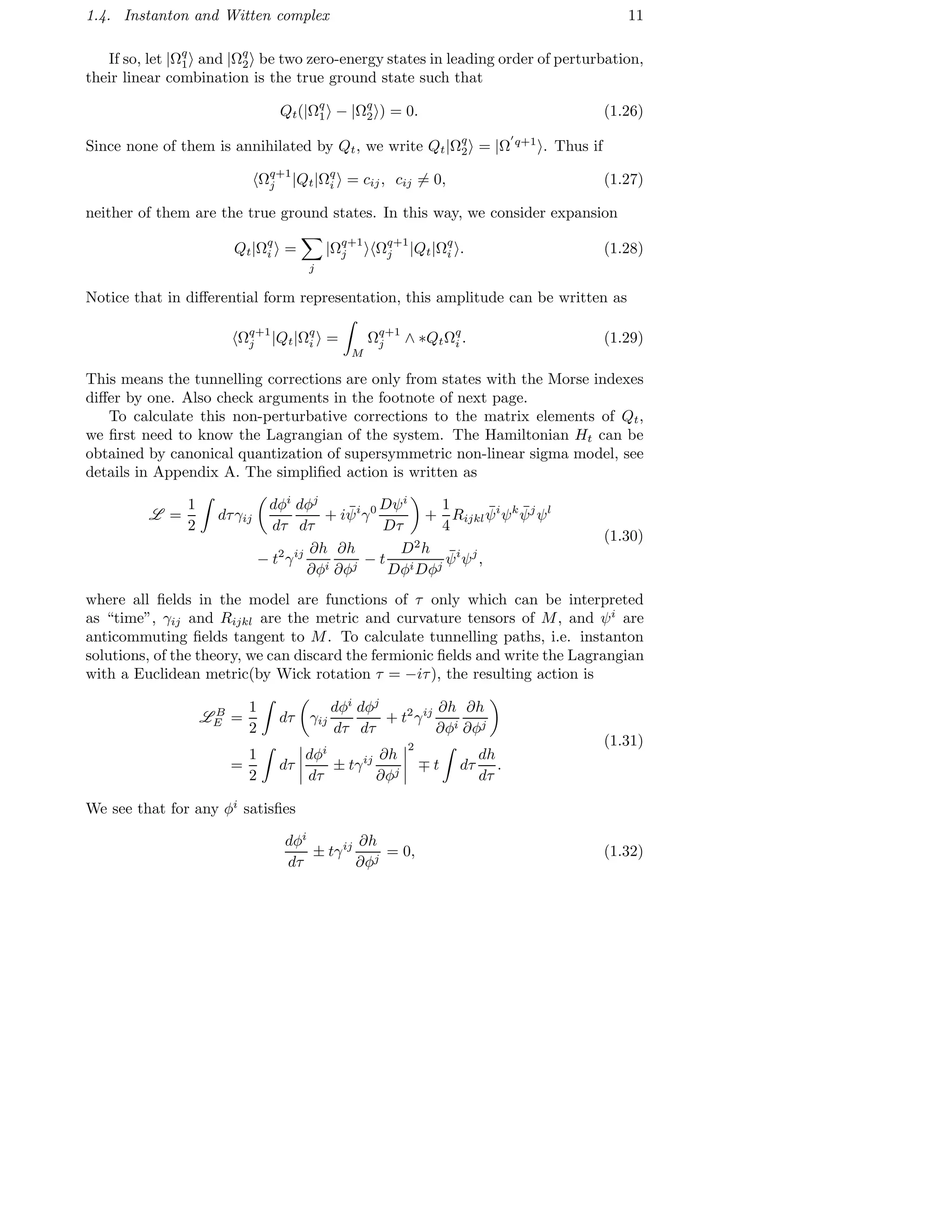
![12 Chapter 1. Supersymmetry and Morse theory
which is the gradient flow of h flowing between critical point Pi with µ−(Pi) = q+1
and critical point Pj with µ−(Pj) = q2
, Eq.(1.31) gives a minimal
¯L = t|h(τ = ∞) − h(τ = −∞)|. (1.35)
Or say for any path, we have
L B
E ≥ t|h(τ = ∞) − h(τ = −∞)|. (1.36)
Configurations that satisfy Eq.(1.32) are called instantons3
. The deformation
of instantons can be obtained by first order variation of this equation as
d
dǫ
d(φi
+ ǫδφi
)
dτ
± tγij
(φi
+ ǫδφi
)∂jh(φi
+ ǫδφi
)
ǫ=0
= D±δφi
:= Dτ δφi
± tγij
Dj∂khδφk
= 0.
(1.37)
Therefore the number of possible deformations is determined by dim ker D±. Ap-
parently, the simplest deformation is given by time translation φ′
(τ) = φ(τ + δτ).
Notice that the eigenfunctions are localized and peaked at corresponding criti-
cal points and rapidly decay upon departing them. However, for two related crit-
ical points4
, their eigenfunctions’ overlap is greatest along the path, solutions of
Eq.(1.32), connecting them. Thus if we consider the Morse function h as an op-
erator which gives the value of h at the corresponding critical point, the desired
amplitude, to the leading order, can be rewritten as path integral
Ωq+1
j |Qt|Ωq
i =
1
h(Pi) − h(Pj) + O(1/t)
lim
T →∞
Ωq+1
j |eT H
[Qt, h]e−T H
|Ωq
i
=
1
h(Pi) − h(Pj)
φj (∞)=Pj
φi(−∞)=Pi
DφDψDψ†
e−LE
ψ†k
∂kh.
(1.38)
2The critical points satisfy boundary conditions φi(−∞) = Pi and φj(∞) = Pj. The gradient
flow is said to be downward flow if the sign in Eq.(1.32) is plus and to be the upward gradient
flow if the sign is minus. Moreover, as mentioned earlier, the non-degenerate Hessian makes us to
separate the tangent space at each critical point into direct sum of two subspaces
TPs M = V +
Ps
⊕ V −
Ps
. (1.33)
By definition µ±(Ps) = dim V ±
Ps
. Accordingly, we can define stable and unstable submanifolds of
M at each critical point Ps as
SPs = {φ| lim
τ→∞
φ(τ) = Ps}
UPs = {φ| lim
τ→−∞
φ(τ) = Ps}.
(1.34)
These submanifolds are tangent to V +
Ps
and V −
Ps
, respectively at Ps. The intersection, UPi
∩ SPj
,
is transverse if the gradient flow of h satisfies the Morse–Smale condition. In this case, if µ−(Pi)−
µ−(Pj) = r, dim UPi
∩ SPj
= r(since µ+(Pj ) = dim M − µ−(Pj ) = dim M − µ−(Pi) + r).
3The name instanton literally infers the transition time is instantly short compare to the
infinite interval of Euclidean time −∞ < τ < ∞.
4As mentioned earlier, only critical points with the Morse indexes differ by one.](https://image.slidesharecdn.com/96310c1d-2d9c-47cc-b2b3-bc64b84ba972-160405111747/75/Thesis-22-2048.jpg)
![1.4. Instanton and Witten complex 13
The operator e−T H
projects states to the perturbative ground states at critical
points Pi. The integral in the second line is obtained by computing [Qt, h] as
[Qt, h]ω = [d + dh∧, h]ω = dh ∧ ω = ψ†k
∂khω. (1.39)
LE in the second line is the Euclidean action. It is combination of the bosonic part
L B
E and the fermionic part L F
E , the later is given by
L F
E =
∞
−∞
dτγij ψ†i
D+ψj
= −
∞
−∞
dτγij D−ψ†i
ψj
. (1.40)
Since the integrand of Eq.(1.38) contains a term ψ†k
∂kh, the amplitude is non-
vanishing only if the number of zero modes of ψ†
is larger than the number of zero
modes of ψ by exactly one. Mathematically, this means that the path integral is
non-vanishing only if
Index D− = dim ker D− − dim ker D+ = 1. (1.41)
One can prove Index D− = ∆µ− := µ−(Pj) − µ−(Pi), since simply speaking the
tunnelling path connects states differ by one fermion only, see more detail in [23].
This again confirms conclusion we had after Eq.(1.29). Importantly, Index D− = 1
ensures that only one instanton deformation exists, which is the shift in τ. This is
the bosonic zero mode. By supersymmetry, we can have only one fermionic zero
mode.
Furthermore, with localization principle, see details in Appendix B, the path
integral localizes to regions where the integral is invariant under some supersym-
metries. Since the Euclidean action is invariant under
δφi
= ǫψ†i
− ¯ǫ
δψi
= ǫ(−
dφi
dτ
+ tγij
∂jh − Γi
jkψ†j
ψk
)
δψ†i
= ¯ǫ(
dφi
dτ
+ tγij
∂jh − Γi
jkψ†j
ψk
),
(1.42)
it is natural to think set all R.H.S. equal to zero. However, we notice that the
integrand is invariant under the ǫ-supersymmetry(generated by Q)
δǫ(ψ†i
∂ih) = 0. (1.43)
Thus we only left with setting the R.H.S. of supersymmetryies
δφi
= ǫψ†i
δψi
= ǫ(−
dφi
dτ
+ tγij
∂jh − Γi
jkψ†j
ψk
)
δψ†i
= 0
(1.44)](https://image.slidesharecdn.com/96310c1d-2d9c-47cc-b2b3-bc64b84ba972-160405111747/75/Thesis-23-2048.jpg)

![1.5. Topological quantum field theory 15
1.5 Topological quantum field theory
Witten’s understanding of relation between supersymmetry and Morse theory is of
great profoundness. It might be the start of golden epoch for modern mathematical
physics. On the other hand, gauge symmetry’s dominating role in particle physics
naturally suggests to find an analogue relation between Morse theory and itself[34].
However, the picture is quite different when we consider the Yang-Mills gauge
theory, the infinite-dimensional space will make the Morse index being ill defined
and also the Morse function itself does not take values in R but R/Z instead.
Thanks for Floer, the work of him on three manifolds[16] significantly changed
the situation. Atiyah first recognized the importance of the work and conjectured
its crucial relations with low-dimensional topologies[1]. In Atiyah’s point of view,
elements of Floer homology are the ground states for a non-relativistic Hamiltonian
in 3-dimensional quantum field theory. Since it is closely related with Donaldson’s
theory of four manifolds[12, 13, 11], the conjecture was concerning a relativistic
generalization. Witten, once again, solved the problem[40] and established the
BRST formulation of topological quantum field theory. We will not get into details
about Floer and Donaldson, but only show the BRST argument of gauge fixing of
CS action.
The construction of Floer is similar to what we have done earlier. In Yang-Mills
gauge theory, the Morse function is called the Chern-Simons function, which we will
start talking in detail from next section. Then one can have the Hamiltonian anal-
ogous to Eq.(1.21). Witten then found that the relativistic Lagrangian corresponds
to the Hamiltonian possesses a fermionic symmetry(supersymmetry generated by
Q), which is quite similar to the BRST symmetry in string theory. The result of it
is of much surprise. Since BRST gauge fixed string action is metric independent,
relativistic generalization of Floer’s theory is a topological quantum field theory.
Let us summarize up. We started to look at supersymmetry as its prominence
of being future particle physics. Its relation to topology, by adding the Morse
function as potential, leads us to topological quantum field theory. The result sur-
prised not only physicists, it also lead mathematicians to relate low dimensional
topologies, especially 3- and 4-dimensions. More recently, mathematical side pays
back that knot invariants give novel understanding of quantization[20, 21]. More-
over, since the CS theory is related to 2-dimensional conformal theories, 2-,3- and
4-dimensional theories are closely related. There are many other interesting facts
following. For example, the localization principle we used in instanton calculation,
it reduces a great ideal of number of integration dimension.](https://image.slidesharecdn.com/96310c1d-2d9c-47cc-b2b3-bc64b84ba972-160405111747/75/Thesis-25-2048.jpg)

![Chapter 2
Chern-Simons
We have skipped a great ideal in last section about topological quantum field theory
as the contents are much beyond the purpose of this thesis. Somehow, it is good to
keep them in mind. Our concentration will now on the Morse function of Floer’s
theory, the Chern-Simons function, as itself is a simple example of topological
theory and the partition function constructed from it can be used to compute knot
invariants, which has deep relation to Floer homology.
Let M be a smooth n-manifold and B be a smooth SU(2) principle bundle over
M with projection π : B → M. The bundle is trivial as B = M × SU(2). The
connection on M is an Lie algebra valued 1-form A. Let A (B) denotes the space of
connections. Since the bundle is trivial, A (B) is isomorphic to Ω1
(M, su(2)), the
space of 1-forms with su(2) coefficients. Let G (B) = C∞
(M, SU(2)) denote the
gauge group, as smooth functions from M → SU(2). Under gauge transformation
g ∈ G (B), the connections A transform according to formula
A −→ Ag = g−1
Ag + g−1
dg. (2.1)
Thus we can define quotient space
C = A /G , (2.2)
as space of gauge equivalent connections.
The Chern-Simons(CS) function is introduced by Chern and Simons. Consider
1-form F = dA + A ∧ A on C given by the curvature. Since it is closed, from the
Bianchi identity, locally it can be written as derivative of some function, that is the
CS function. The definition is as follow, let A0 be the trivial connection and put
At = (1 − t)A + tA0 for 0 ≤ t ≤ 1. This is a connection on M × [0, 1]. Now define
CS(A) =
1
8π M×[0,1]
Tr F2
, (2.3)
where F is the curvature on M × [0, 1]. Notice that the integral on a closed 4-
manifold gives π times the second Chern class. Moreover, the CS function is a
17](https://image.slidesharecdn.com/96310c1d-2d9c-47cc-b2b3-bc64b84ba972-160405111747/75/Thesis-27-2048.jpg)

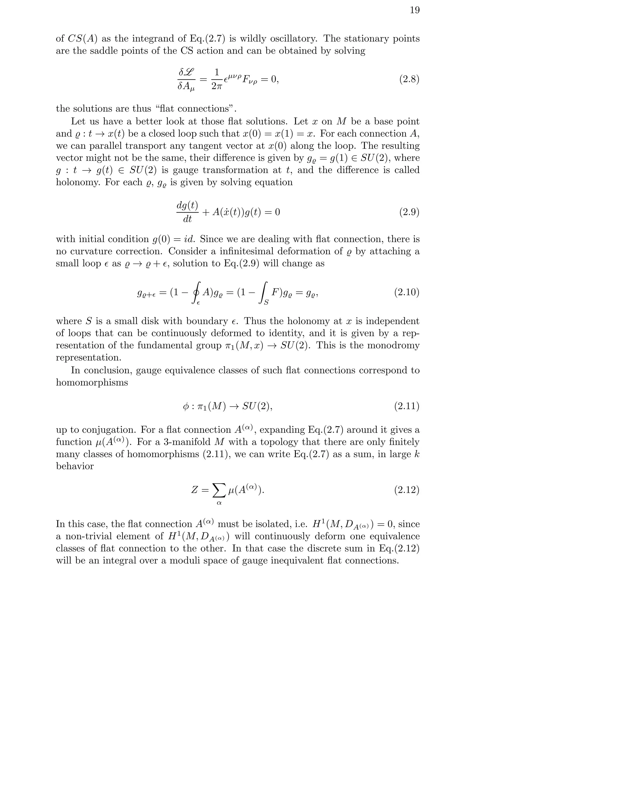

![2.2. Twisted de Rham cohomology 21
perturb around the flat connection by rewriting A = A(α)
+ B. Therefore the
differential operator will be a covariant derivative DA(α) . It acts on B as
DA(α) B = dB + [A(α)
, B]. (2.17)
Since the covariant derivative DA(α) is respect to the flat connection A(α)
,
D2
A(α) = FA(α) = 0. We can write down a complex
0 → Ω0
(M, su(2))
DA(α)
−−−−→ Ω1
(M, su(2))
DA(α)
−−−−→
Ω2
(M, su(2))
DA(α)
−−−−→ Ω3
(M, su(2)) → 0.
Notice that Ω0
(M, su(2)) is the Lie algebra of SU(2) gauge transformations, that
is if we write the gauge transformation as g = eiφ
then φ ∈ Ω0
(M, su(2)). They
generator infinitesimal gauge transformations.
With a metric on M, we can define the Hodge star as an operator maps from ∗ :
Ωq
(M, su(2)) → Ωn−q
(M, su(2)). This enable us to have a pairing on Ωq
(M, su(2))
as
b, b ≡ −
M
Tr(b ∧ ∗b), (2.18)
where b is Lie algebra valued q-form. With pairing we can define the dual operator
D†
A(α) : Ωq
(M, su(2)) → Ωq−1
(M, su(2)) by equation
D†
A(α) = (−1)n(p+1)+1
∗ DA(α) ∗, (2.19)
where n = 3 in our case.
Consider a ∈ KerDA(α) , then one has
DA(α) a, φ = a, D†
A(α) φ = 0, ∀φ ∈ Ω1
(M, su(2)), (2.20)
where D†
A(α) = − ∗ DA(α) ∗, thus the equality
(KerDA(α) )⊥
= ImD†
A(α) . (2.21)
Therefore we have the basic orthogonal decomposition3
,
Ω0
(M, su(2)) = KerDA(α) ⊕ ImD†
A(α) , (2.22)
similarly, it is readily to obtain
Ω1
(M, su(2)) = KerD†
A(α) ⊕ ImDA(α) . (2.23)
3The Hodge decomposition.](https://image.slidesharecdn.com/96310c1d-2d9c-47cc-b2b3-bc64b84ba972-160405111747/75/Thesis-31-2048.jpg)

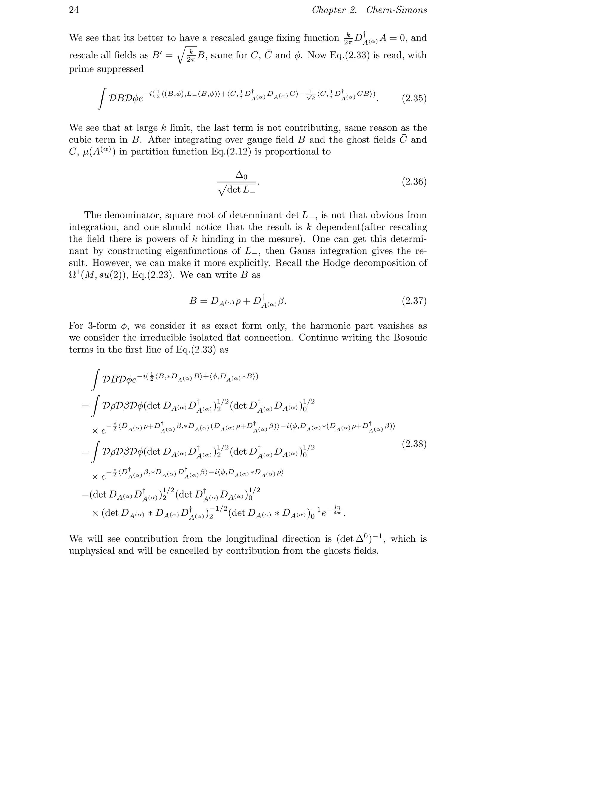
![2.3. First loop correction 23
where C, ¯C ∈ (KerDA(α) )⊥
. It can be divided into a kinetic term of ghosts plus an
interaction term between the ghost fields and the fluctuation B as
¯C, D†
A(α) DA(α)+BC
= ¯C, D†
A(α) DA(α) C + ¯C, D†
A(α) [B, C]
= ¯C, D†
A(α) DA(α) C + ¯C, D†
A(α) BC − ¯C, D†
A(α) CB
= ¯C, D†
A(α) DA(α) C − ¯C, D†
A(α) CB .
(2.30)
On the other hand the delta constraint can also be expressed by integral
δ(D†
A(α)
A) = Dφe
−i Tr(φ∧D†
A(α)
A)
= Dφei Tr(φ∧DA(α) ∗A)
= Dφe−i φ,DA(α) ∗A
,
(2.31)
where φ is a 3-form, bosonic field.
Now we are ready to check the total gauged Lagrangian. Put Eq.(2.27) together
with gauge constrain Dgδ(D†
A(α) ) into L (A), and if we consider change of variable
A = A(α)
+ B, in which B is perturbation around flat connection A(α)
, expanded
Lgauged(A)5
reads
Lgauged(A) = L (A(α)
) +
k
4π M
Tr( B ∧ DA(α) B + φ ∧
4π
k
D†
A(α) B
+ ¯C ∧ ∗
4π
ik
D†
A(α) DA(α) C − ¯C ∧ ∗
4π
ik
D†
A(α) CB).
(2.32)
Combining the dynamical term of B , we have the integrand written as
e
−i k
4π ( B,∗DA(α) B + φ, 4π
k DA(α) ∗B + ¯C, 4π
ik D†
A(α)
DA(α) C − ¯C, 4π
ik D†
A(α)
CB )
=e
−i k
4π ( (B,φ),L−(B,φ) + ¯C, 4π
ik D†
A(α)
DA(α) C − ¯C, 4π
ik D†
A(α)
CB )
,
(2.33)
where we have write the pair (B, φ) as a two component vector, and L− = (DA(α) ∗
+∗DA(α) )ǫ, where ǫψ = ψ for ψ ∈ Ω1
(M, su(2)) and ǫψ = −ψ for ψ ∈ Ω3
(M, su(2)),
is a self-dual operator, maps within forms of odd order, given by
L− =
∗DA(α) −2π
k DA(α) ∗
2π
k DA(α) ∗ 0
(2.34)
5The gauged Lagrangian possesses BRST symmetry, and it is metric independent. See details
in Appendix F](https://image.slidesharecdn.com/96310c1d-2d9c-47cc-b2b3-bc64b84ba972-160405111747/75/Thesis-33-2048.jpg)
![26 Chapter 2. Chern-Simons
We have used identities6
. This agrees with Rozansky[31]. Denote the Ray-Singer
torsion at level k as τ = ( k
4π2 )−1/2(ζ(0,∆0)−ζ(0,∆1)) (det ∆0)3/4
(det ∆1)1/4 . Recall that there is
k dependence hidden in the integration measure after rescaled all fields, and the
results of rescaled and non-rescaled cases must be consistent. As zeta regulariza-
tion removes all zero modes, a factor ( k
4π2 )−1/2(dim H0
(M,DA(α) )−dim H1
(M,DA(α) ))
is
needed to account for the k dependence of zero modes7
.
Later in this section, we will see this ratio is exactly the analytic Ray-Singer
torsion of DA(α) , after zeta regularization of these determinants, see details about
Ray-Singer torsion in Appendix C. This torsion is topologically invariant which
means the gauged Lagrangian must be metric independent. On the other hand,
a similar problem appears that Lgauge’s dependence on gauge fixing functional
may ruin gauge invariance of the theory. Fortunately, a continues symmetry ,which
related to gauge invariance, of Lgauge was discovered by Becchi, Rouet, and Stora[8]
(independently by Tyutin[35]) in 1975, and is known in honor of its discoverers as
BRST symmetry. BRST symmetry was originally found in string theory, it features
general covariance, thus topological. In Appendix F, we use BRST symmetry to
demonstrate the topological feature of gauge CS action.
6Here we need three identities. If one has self-dual operator K, the relation det |K| =
(det K2)1/2 = (det K†K)1/2 is trivial and we can write
(det
ik
4π2
DA(α) ∗ DA(α) ǫD†
A(α) )
−1/2
2
=(det(
k
4π2
)2
DA(α) ∗ DA(α) ǫD†
A(α)
DA(α) ∗ DA(α) ǫD†
A(α)
)
−1/4
2
=(det(
k
4π2
)2/3
DA(α) D†
A(α) )
−3/4
2
(2.42)
Recall [∆, D] = 0, also true for the twisted operator DA(α) , and act it on a q − 1-form ωq−1 from
both side, we have
Dq−1∆q−1(D†
qωq + Dq−2ωq−2) = ∆qDq−1(D†
qωq + Dq−2ωq−2). (2.43)
We see that the eigenvalues of ∆q−1 restricted to co-exact eigenmodes are same as the
eigenvalues of ∆q restricted to exact eigenmodes. This means det D†
qDq−1 = det Dq−1D†
q.
Furthermore, orthogonality of the Hodge decomposition leads to the relation det ∆q =
(det D†
q+1Dq)(det Dq−1D†
q). One can prove this by considering the zeta invariant of ∆ given
by
ζ(s, ∆) = ζ(s, D†
q+1Dq) + ζ(s, Dq−1D†
q), (2.44)
and the determinant of Laplacian is
det ∆q =e−ζ′(0,∆q)
=e
−ζ′
(0,D
†
q+1Dq)
+ e−ζ′
(0,Dq−1D†
q)
=(det D†
q+1Dq)(det Dq−1D†
q)
(2.45)
7This factor is indeed for general cases. In our situation, isolated connection indicates
dim H1(M, DA(α) )) = 0. In most simple case, irreducible isolated connection Witten first consid-
ered, there is no such factor.](https://image.slidesharecdn.com/96310c1d-2d9c-47cc-b2b3-bc64b84ba972-160405111747/75/Thesis-36-2048.jpg)
![2.4. Regularization 27
2.4 Regularization
The determinants in Eq.(2.75) might not be well defined as there are infinite many
eigenvalues. An appropriate regularization is needed. Consider a Laplace operator
∆ with positive eigenvalues λ, one can define the zeta function
ζ(s, ∆) =
λ
λ−s
= Tr ∆−s
. (2.46)
When Re(s) is sufficiently large, zeta function is meromorphic. Schwarz showed
in [32] that it can be analytically continued to the whole complex plane, in which
s = 0 is not a pole and ζ(0, ∆) and ζ′
(0, ∆) are well defined. From this definition,
ζ(0, ∆) is the dimension of the Hilbert space, only for even dimensions. Ray and
Singer[30] showed that one can define
det ∆ = e−ζ′
(0,∆)
, (2.47)
since
ζ′
(0, ∆) =
λ
d
ds
λ−s
|s=0
=
λ
− log λ.
(2.48)
This definition results det ∆ as a real number, and is exactly what we want from a
Gaussian integration. On the other hand the sign of operator in the phase term of
Eq.(2.16) can be given by the eta-function which for a self-adjoint linear operator
K (may have both positive and negative eigenvalues) is defined as
η(s, K) =
k
1
(λ
(+)
k )s
−
l
1
(λ
(−)
l )s
, (2.49)
where λ
(+)
l and λ
(−)
l are the strictly positive and negative eigenvalues of K, re-
spectively. With this regularization scheme, the determinants are well defined. We
actually already used this regularization in deriving the result, as one can see the
k dependent factor is coming from this procedure8
, Eq.(2.75). Moreover, Ray and
Singer[30] proved that
TA(α) =
(det ∆0
A(α) )
3
4
(det ∆1
A(α) )
1
4
(2.50)
is topological invariant. Therefore the 1-loop correction of the CS theory is topolog-
ical invariant. See more details about how to define Ray-Singer torsion in Appendix
C.
8In literatures, some authors intend to use det′
∆ to denote the regularized determinant.](https://image.slidesharecdn.com/96310c1d-2d9c-47cc-b2b3-bc64b84ba972-160405111747/75/Thesis-37-2048.jpg)
![28 Chapter 2. Chern-Simons
2.5 The eta invariant
The eta invariant η(0, L−) is defined to see the spectral asymmetry of operators9
.
We want to know its dependence on the background field A(α)
, and write η(A(α)
)
instead later on. Before getting complicated we start with a simple example. Sup-
pose we have a particular operator with eigenvalues λm = m + a, m ∈ Z and
0 < a < 1. With zeta regularization we have the spectral asymmetry as
ηa = lim
ǫ→0
(
λm>0
e−λmǫ
−
λm<0
eλmǫ
)
= lim
ǫ→0
(
e−aǫ
1 − e−ǫ
−
e−(1−a)ǫ
1 − e−ǫ
)
= 1 − 2a.
(2.51)
We see this non-trivial dependence of ηa on a since numbers of positive and negative
λ of different a ∈ (0, 1) are not same. Moreover, since m ∈ Z ηa is periodic, i.e.
ηa = ηa+n, n ∈ Z. We can consider variation of a within (0, 1) as continuous
dependence of ηa on a. When a passes through an integer n, λ−n changes sign and
we recognize this as discontinuous dependence of ηa on a. Then we can write ηa
for any a as
ηa = 1 − 2a − 2SFa, (2.52)
where SFa is the discontinuous jump called spectral flow and the factor 2 comes as
once an eigenvalue changes sign ηa jumps by 2 units. If we define zero eigenvalues
as positive, η0 = 1 as number of positive eigenvalues is the same as of negative
eigenvalues and we have
ηa = η0 − 1 + (1 − 2a) − 2SFa
→ ηa − η0 = cont.0→a − 2SFa.
(2.53)
Now we can proceed to analyse η(A(α)
). For trivial connection, the zero modes
are easy to count. Recall operator L− is acting on zero and 1-forms, thus zero
modes are constant Lie algebra valued functions and Lie algebra valued closed 1-
forms, i.e. (1 + b1
(M)) dim G. However, from the second line of Eq.(2.53) we see
that it is not important to know the zero modes, especially in simplest case there
is no zero modes. The crucial observation is their difference compares to “1 − 2a”.
This difference is the continuous dependence of A(α)
, and it can be written by a
local expression. To see this explicitly, a rigorous derivation refers to [9], we will
start with an observation from Mellin transformation
1
2
Γ(
s + 1
2
)t−(s+1)/2
=
∞
0
dyys
e−ty2
, t > 0. (2.54)
9This phase term is induced by existing of both positive and negative eigenvalues.](https://image.slidesharecdn.com/96310c1d-2d9c-47cc-b2b3-bc64b84ba972-160405111747/75/Thesis-38-2048.jpg)
![2.5. The eta invariant 29
Notice that if we change variable t = x2
, it becomes
x−s
=
2
Γ(s+1
2 )
∞
0
dyys
xe−x2
y2
→ |x|−s
sign x =
2
Γ(s+1
2 )
∞
0
dyys
xe−x2
y2
,
(2.55)
where the first line obviously detects the sign of x, and thus the second line is valid.
The eta invariant of operator L− with arbitrary gauge field A can be written as
η(s, L−) =
2
Γ(s+1
2 )
∞
0
dyys
Tr(L−e−y2
L2
− ), (2.56)
where the trace is over all eigenvalues of L−. The eta invariant is well defined at
s = 0 in our case, and one can write
η(L−) =
2
√
π
lim
s→0
∞
0
dyys
Tr(L−e−y2
L2
− ). (2.57)
Under an arbitrary variation of A, we have
δη(L−) =
2
√
π
lim
s→0
∞
0
dyys
Tr((δL− − 2y2
δL− · L2
−)e−y2
L2
− )
=
2
√
π
lim
s→0
∞
0
dyys d
dy
(y Tr(δL−e−y2
L2
− )).
(2.58)
Integrating by parts, setting s → 0 and evaluating boundary term at y = 0, we
have
δη(L−) =
2
√
π
lim
y→0
(y Tr(δL−e−y2
L2
− )), (2.59)
such limit might not be rigorous. In general case, one has to picking out the
coefficient of y−1
in the small y expansion of Tr(e−y2
L2
− )[9].
To see how the variation works, we first separate the operator into components.
For local coordinates xi
on M, a differential operator DA coupled with gauge field
A acts on a q-form ω as
DAω = dω + A ∧ ω
= ∂iω ∧ dxi
+ Aidxi
∧ ω
= ψi
∂iω + ψi
Aiω
= ψi
Diω
(2.60)
One can see the operator ψi
maps a → a ∧ dxi
. Also there is a dual operation
associated with it
∗ψi
∗ = (−1)F
χi
, ∗χi
∗ = ψi
(−1)F
, (2.61)](https://image.slidesharecdn.com/96310c1d-2d9c-47cc-b2b3-bc64b84ba972-160405111747/75/Thesis-39-2048.jpg)
F
∗DAǫDA ∗ ǫ = −
1
2
χi
χj
[Di, Dj](−1)F
DA ∗ ǫDA ∗ ǫ + ∗DAǫ ∗ DAǫ = DiDi
,
(2.63)
we can write it as L2
− = −(X − ∆) with
X =
1
2
(ψi
ψj
[Di, Dj](−1)F
+ χi
χj
[Di, Dj](−1)F
). (2.64)
Now we can use expansion
e−y2
∆
ey2
X
= e−y2
∆
+
y2
0
dse−s∆
Xe−(y2
−s)∆
+ . . . , (2.65)
and the Zassenhaus formula
ey2
(−∆+X)
= e−y2
∆
ey2
X
e− y4
2 [−∆,X]
e
y8
6 (2[X,[−∆,X]]+[−∆,[−∆,X]]
· · · (2.66)
to rewrite
ey2
(−∆+X)
→ y2
Xe−y2
∆
. (2.67)
The fact that we can do this is because when taking the limit y → 0, only the second
term in expansion Eq.(2.65) survives. Moreover, we can see from the Zassenhaus
formula that non-commutative part of X and ∆ have higher orders in y2
, thus the
assumption that non-commutative part does not contribute ensure this rewrite is
legitimate. The assumption will be assured by evaluating e−y2
∆
with help of the
heat kernel method. With the standard heat kernel expansion
e−y2
∆
∼ (4π)−3/2
s
ys−3
bs, (2.68)
we see that the lowest power in y is −3. Therefore any higher order in y2
will be
zero within the limit y → 0. On the other hand, other terms not vanishing after the
limit will be zero by taking trace in Eq.(2.59). Gather all the steps above, Eq.(2.59)
can be written as
δη =
1
4π2
Tr(δL− · X). (2.69)
Since the Hodge star ∗ maps odd forms to even forms and even forms to odd
forms in 3-dimension and it does not change the eigenvalues, we can consider](https://image.slidesharecdn.com/96310c1d-2d9c-47cc-b2b3-bc64b84ba972-160405111747/75/Thesis-40-2048.jpg)
![2.5. The eta invariant 31
L− which acts on Ω1
(M, su(2)) ⊕ Ω3
(M, su(2)) as ∗DAǫ acts on the total space
Ω•
(M, su(2)). Thus
δη =
1
4π2
M
˜Tr(∗δDAǫ · X), (2.70)
where the trace is over Ω•
(M, su(2)). Notice that every term in X is quadratic in
χi
and ψj
, and δDA = ψi
δAi, hence if we denote χi
and ψi
both as γi
we have
˜Tr ∗ ψi
ǫγj
γk
= εijk
, (2.71)
where εijk
is the Levi-Civita antisymmetric tensor. Since the space Ω∗
(M, su(2)) is
Lie algebra valued, we still have the trace over su(2) in the adjoint representation
left10
and
δη =
1
8π2
M
εijk
Trsu(2)(4δAi[Dj, Dk])
=
−1
π2
M
Trsu(2)(δA ∧ dA + δA ∧ A ∧ A).
(2.72)
Notice that the minus sign in second line is caused by the pairing eq.(2.18), thus
one should bear in mind the eta invariant is respect to this pairing. We can take
A as our background field A(α)
. After integration, the continuous dependence of
η(A(α)
) is given by
˜η(A(α)
) =
−1
2π2
M
Trsu(2)(A(α)
∧ dA(α)
+
2
3
A(α)
∧ A(α)
∧ A(α)
)
=
−2c2(SU(2))
π
CS(A(α)
),
(2.73)
where c2(G) is the value of the quadratic Casimir operator of G in the adjoint
representation(c2(SU(N)) = 2N, see Eq.(3.63) and Eq.(3.69) for detail), CS(A(α)
)
is the CS invariant of flat connection A(α)
.
In conclusion, η(A(α)
) in the phase term of the one-loop correction can be writ-
ten as
η(A(α)
) = η(0) −
2c2(G)
π
CS(A(α)
) − 2SFA(α) . (2.74)
Again, this is the formula for general cases. The problem of this formula is that
only η(0) is not topological. Now we can write the partition function at 1-loop
correction of flat connection A(α)
as
Zα =
1
VolHα
eiπη(0)/4−iπSFA(α) /2
(
k
4π2
)−1/2 dim H0
(M,DA(α) )
(2.75)
ei(k+
c2(SU(2))
2 )CS(A(α)
)
TA(α) .
10Notice that the path integral Eq.(2.33) is over perturbation B which transforms in adjoint
representation under gauge symmetry. Thus the trace left with is in adjoint representation in-
stead of the fundamental one. However they differ by a quadratic Casimir of the SU(2) adjoint
representation.](https://image.slidesharecdn.com/96310c1d-2d9c-47cc-b2b3-bc64b84ba972-160405111747/75/Thesis-41-2048.jpg)
![32 Chapter 2. Chern-Simons
For isolated irreducible flat connection ( k
4π2 )−1/2 dim H0
(M,DA(α) )
= 1, VolHα = 1
and SFA(α) = 0. To get rid of the metric dependence for η(0), Witten in [42] added
a gravitational CS functional(definition in Appendix D) to cancel it. This operation
requires a trivialization of the tangent bundle of M. Different trivializations only
differ in a number of “twists”, which is the framing dependence. Thus there is an
overall phase factor
eiπd(ηgrav/4−CS(ω)/24π)
=e−2πidσ(µ)/8
,
(2.76)
where d = dim SU(2), dηgrav = η(0), and define σ(µ) as the overall factor depends
on framing. The theory finally gives topologically invariant result with a specific
framing choice. In addition, Atiyah showed that there always exists a canonical
2-framing µ such that σ(µ) = 0 [2].
2.6 Metric dependence of η(0)
To understand the detail about the framing dependence of the CS theory, we first
start with Atiyah-Patodi-Singer theorem and see why η(0) is metric dependent. The
original purpose of the theorem is to have a generalization of Hirzebruch’s signature
theorem of manifolds with boundary. Let W be a compact manifold with boundary
Y and D : C∞
(W, E) → C∞
(W, F) be a linear first order elliptic differential
operator acting from vector bundle E to vector bundle F over W. Assuming that,
in a neighbourhood Y × [0, 1] of the boundary, D has the form D = ∂u + A, where
u is the inward normal coordinate to the boundary and A : E|Y → F|Y is elliptic
self-adjoint operator on Y . Then one can write a finite index of D as
index D =
W
α0dx −
h + η(A)
2
, (2.77)
where α0 is some characteristic polynomial obtained from the constant term in the
asymptotic expansion of the heat kernel e−tD†
D
− e−tDD†
. In the case of operator
L, recall L− is the restriction to odd forms, α0 is given by[3]
α0 = −π−2
Tr[F2
] +
2
3
p1, (2.78)
and we can consider it as twice the continuous part of η(A(α)
). The second term
comes from boundary condition. An interesting point is that this term only de-
pends on Y as one can glue W′
with opposite orientation to W along Y . With
suitable example of lens space, this indicates the boundary term must be a global
invariant of metric on Y [4]. Surprisingly η invariant separates the spectrum of A
into positive and negative parts and such non-local character is exactly what we
want for the boundary condition. This also explain the reason that η(0) is metric](https://image.slidesharecdn.com/96310c1d-2d9c-47cc-b2b3-bc64b84ba972-160405111747/75/Thesis-42-2048.jpg)
![2.7. 2-framing of 3-manifold 33
dependent. h in the second term is the multiplicity of zero eigenvalues of D on Y ,
h = (dim H0
(Y, D) + dim H1
(Y, D) + dim H2
(Y, D) + dim H3
(Y, D)).
Freed and Gompf used this theorem to calculate η(A(α)
)[17]. By putting A(α)
and trivial connection to the ends of Y × [0, 1], separately, the APS theorem gives
exactly same result as Eq.(2.74). The only thing one has to take care is that D is
not restricted to odd forms, i.e η(A) = 2η(A(α)
), when applying the APS theorem.
2.7 2-framing of 3-manifold
Given a manifold, we are wondering whether it is plausible to have a same basis at
each point, that is whether one can find a global section to trivialize the tangent
bundle. For this reason one constructs a frame bundle over the base manifold, and
at each point the bundle consists all local basses. Suppose we have a section of
the frame bundle, it gives a trivialization of the tangent bundle. To ensure the
trivialization is globally defined, we have to first make sure it is extendible from
0-skeleton to 1-skeleton. This is indeed the definition of orientation, that is for
an oriented 3-manifold Y , the extension is trivial. An orientation is specified by
its homotopy class. Moreover, analogous to orientation we define spin structure.
In this scenario Y admits spin structure if the trivialization can be extended over
the 2-skeleton. For oriented 3-manifold, one can always find such globally defined
trivialization and the manifold is called parallelizable. However, the choice of trivi-
alization of its tangent bundle is not unique. This arouses the definition of framing
of 3-manifold, a choice of trivialization of the tangent bundle of Y . Two different
trivializations are related by the transition function, thus it can be characterized by
the map Y → SO(3). Since Y is oriented, the first Stiefel-Whitney class vanishes,
ω1(Y ) = 0. Since the tangent bundle of Y has structure group SO(3) and the
Stiefel-Whitney classes ω1(Y ) = 0, we can lift map Y → SO(3) to Y → SU(2)
if and only if ω2(Y ) = 0, i.e. Y admits a spin structure. Different framings of
Y is thus characterized by homotopy classes of this map11
. However, there is an-
other more interesting integer we can define, called the 2-framing of Y , which is
introduced by Atiyah in [2].
Let TY denotes tangent bundle of Y , we can define a direct sum 2TY = TY ⊕TY .
Consider a diagonal embedding map
SO(3) → SO(3) × SO(3) → SO(6), (2.79)
11From standard obstruction theory when one wishes to expend a trivialization from 0-skeleton
over 1-skeleton, the obstruction is coming from ω1 ∈ H1(Y, π0(SO(3)). To extend over 2-skeleton,
the obstruction is coming from ω2 ∈ H2(Y, π1(SO(3)). Thus if both ω1 and ω2 are zero, one
can change the SO(3) bundle to SU(2) bundle which is a double over of SO(3). It is readily
seen that H1(Y, π0(SU(2)) and H2(Y, π1(SU(2)) vanish trivially as SU(2) is 2-connected, thus a
globally defined trivialization of SU(2) bundle exists. Different trivialization is within homotopy
class of map Y → SU(2). Since we are within 3-dimension, this map is indeed the degree map
that different homotopy classes are characterized by the number of times the map wraps over Y .](https://image.slidesharecdn.com/96310c1d-2d9c-47cc-b2b3-bc64b84ba972-160405111747/75/Thesis-43-2048.jpg)

![2.7. 2-framing of 3-manifold 35
Naively, by using Stokes theorem
Y ×I
Tr F2
=
Y
Tr(AdA +
2
3
A3
), (2.83)
we can consider the degree of θµν as the difference between non-trivial gauge trans-
formations of the CS functional, i.e. the last term of Eq.(2.5). Indeed it is an
integer. To be precise, we first cover W with coordinates patches UI, on which
2TY is trivialized. Locally, we can always define connection over Ui, and glue them
together with the partition of unity {ρi} as
Ai =
j
ρjt−1
ji dtji, (2.84)
where tij is the transition function. If we write tij = tiktkj, the formula of gauge
transformation is recovered
Ai =
j
ρj(tjktki)−1
d(tjktki)
= t−1
ki (
j
ρjt−1
ki dtki)tki +
j
ρjt−1
ki dtki
= t−1
ki Aktki + t−1
ki dtki.
(2.85)
In our case, 2TY is trivialized by µ and ν on U1 and U2, respectively, hence the
transition function is t = θ−1
µν . Accordingly, we can write connections as
A1 = ρ2t−1
dt, A2 = ρ1tdt−1
, ρ1 + ρ2 = 1. (2.86)
The curvature is given by
F1 = dA1 + A1 ∧ A1
= dρ2t−1
dt + (ρ2
2 − ρ2)(t−1
dt)2
.
(2.87)
Now the degree of θµν is calculated as
deg(θµν) =
1
2 Y ×I
ˆp1(2TW )
=
1
8π2
Y ×I
2dρ2(ρ2 − ρ2
2) Tr[(t−1
dt)3
]
=
1
24π2
Y
Tr[(θ−1
µν dθµν)3
].
(2.88)
Now consider Fig.(2.1(b)), in this scenario M1 is an oriented 4-manifold with
boundary Y . Given any 2-framing µ of Y we can define
σ(µ) = SignM1 −
1
6 M1
ˆp1(2TM1 , µ), (2.89)
where SignM1 is the Hirzebruch signature. The definition here makes sense since we
can consider σ(µ) as the boundary condition to the generalized Hirzebruch signature](https://image.slidesharecdn.com/96310c1d-2d9c-47cc-b2b3-bc64b84ba972-160405111747/75/Thesis-45-2048.jpg)

![Chapter 3
Non-perturbative
comparison
We will compare the 1-loop correction with exact result in this section. The reason
besides evaluating the validity of perturbative method are that this leads to the
first example of AdS3/CFT2. The main tool to compute the CS partition function
is the affine Lie algebra introduced by Kac[24]. We will first give a brief review
of representation theory of Lie algebra and see how to calculate the character of
it. Then extend to the case of affine Lie algebra and we will see its connection to
conformal field theory.
3.1 Weyl character formula
Let G be a Lie group and ta (a = 0, . . . , dim G) be its group generators. The
commutation relations of ta define its Lie algebra g. We will focus on semi-simple
Lie algebra which is a direct sum of simple Lie algebra1
. Most simple example of
non-semisimple group is U(n) = U(1)×SU(n) since U(1) is the non-trivial Abelian
subalgebra, and we see that SU(n) is semisimple.
Let V be representations of G on complex vector spaces, its characters are
defined as functions
χV : g ∈ G → Tr(V (g)) ∈ C, (3.1)
and they are invariant under conjugation
χ(g′
gg′−1
) = χ(g) g′
∈ G. (3.2)
1g is simple if it has no non-trivial Abelian subalgebra. The generators of such subalgebra
commute with all other generators of g.
37](https://image.slidesharecdn.com/96310c1d-2d9c-47cc-b2b3-bc64b84ba972-160405111747/75/Thesis-47-2048.jpg)
![38 Chapter 3. Non-perturbative comparison
Moreover, the character characterizes the associated representation up to isomor-
phism. Consider G = U(1), the irreducible representations are one dimensional
with integer label n. The character is given by
χ(eiθ
) = einθ
. (3.3)
Let Ha
(a = 0, . . . , rankG) be linearly independent generators of g that com-
mute within themselves
[Ha
, Hb
] = 0, a, b = 1, . . . , rank G. (3.4)
{Ha
} forms a maximal Abelian subalgebra h of g, i.e. the Cartan subalgebra. The
Lie group of h is denoted as T , a maximal torus of G. We can consider the maximal
torus as a finite product of k copies of U(1) and its irreducible representations are
labelled by k integers. The importance of maximal torus is that any element g ∈ G
can be conjugated into an element of T 2
. Therefore a conjugation invariant func-
tion, e.g. χV , is determined by its values on T . Since the characters of irreducible
representations of T are known, it is plausible to determine that of G.
To achieve this goal, we begin with denoting other generators of g as Eα
and
their commutation relations with Ha
[Ha
, Eα
] = αa
Eα
, a = 1, . . . , rank G = r. (3.5)
The eigenvalues αa
, the Dynkin labels, form a r-dimensional vector space and is
called a root of g. The root α is called a positive root if its first component is posi-
tive. We can choose a basis for this r-dimensional vector space as {α(a)
} and each
α(a)
is called a simple root. With this set up, we have the Cartan decomposition
of g
g = h ⊕ g+ ⊕ g−. (3.6)
For semi-simple Lie groups, their Killing forms are non-degenerate. Thus it can
help us to define an inner product ·, · on Cartan subalgebra h
K(Ha
, Hb
) = 2
c
α(c)
, α(a)
α(c)
, α(b)
α(a), α(a) α(b), α(b)
. (3.7)
In addition, we can define the r × r Cartan matrix and its entries are given by
Aab
= 2
α(a)
, α(b)
α(b), α(b)
. (3.8)
If we define the dual root or coroot of α by
α∨
=
2α
α, α
, (3.9)
2Indeed, this is the main theorem of maximal torus. For detail poof, we refer interested reader
to look into formal text books on Lie group representation theory, e.g. [10].](https://image.slidesharecdn.com/96310c1d-2d9c-47cc-b2b3-bc64b84ba972-160405111747/75/Thesis-48-2048.jpg)

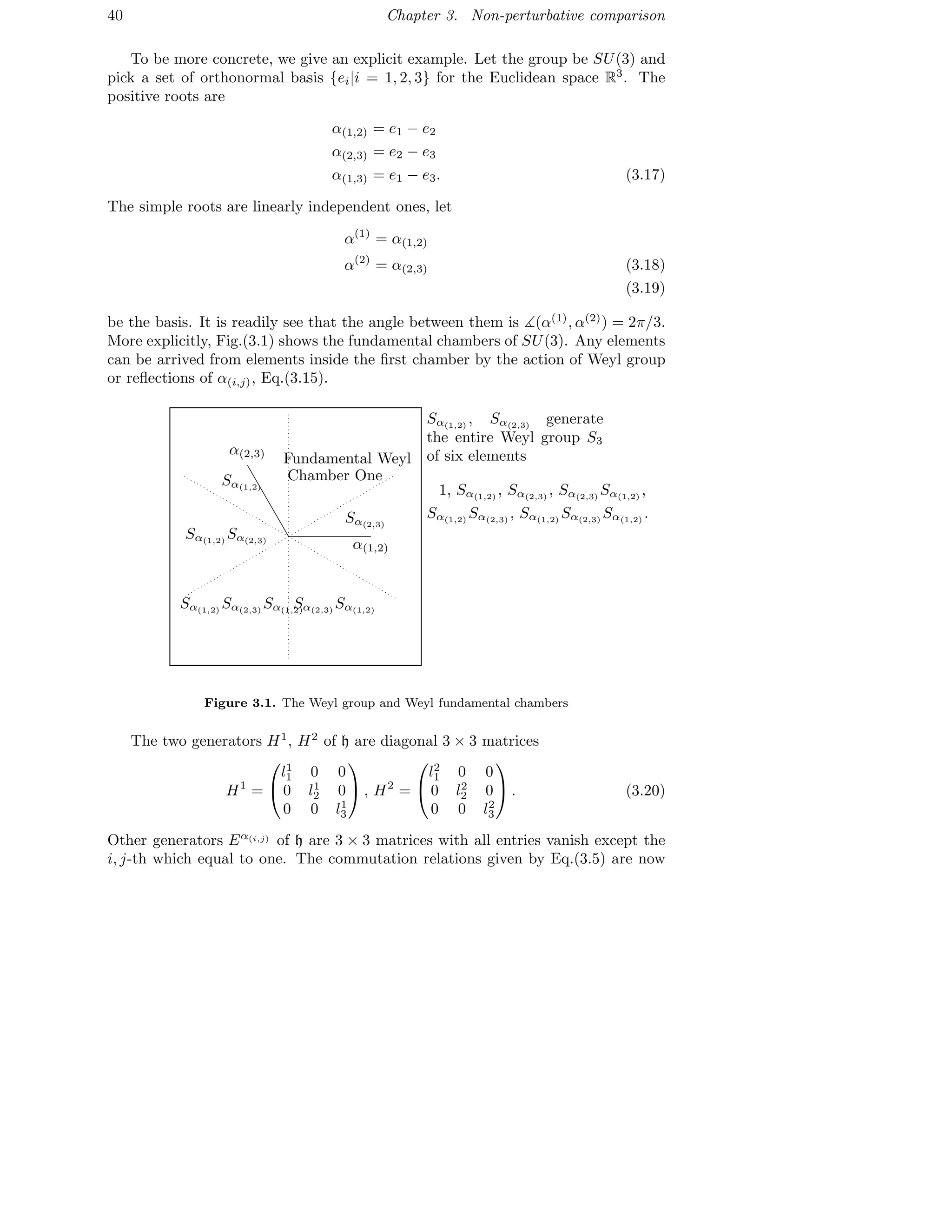
![3.1. Weyl character formula 41
written as,
[H1
, Eα(i,j)
] = (l1
i − l1
j )Eα(i,j)
, [H2
, Eα(i,j)
] = (l2
i − l2
j )Eα(i,j)
. (3.21)
Now the components of root α(i,j) in the basis of fundamental weights Λ(i) are given
by the eigenvalues, the Dynkin labels, of these commutation relations
α(i,j) = (la
i − la
j )Λ(a) = α(i,j)(Ha
)Λ(a), (3.22)
where α(i,j)(Ha
) denotes the inner product of α(i,j), Ha
in the Euclidean basis ei.
For example,
α(1)
= 2Λ(1) − Λ(2), α(2)
= −Λ(1) + 2Λ(2). (3.23)
Moreover, the Cartan matrix is computed as
A =
2 −1
−1 2
(3.24)
by Eq.(3.8).
One can see theses relation explicitly in Fig.(3.2). The highest weights are
living in the fundamental Weyl chamber one. We point out three of them, in Λ(i)
basis, and how they transform under the Weyl group. The red line represents the
(1, 0) fundamental representation of SU(3) which is the defining representation on
R3
, the highest weight is Λ(1). The blue line represents the (0, 1) fundamental
representation of SU(3) which is the wedge product representation on ∧2
(R3
), the
highest weight is Λ(2). The green line represents the adjoint representation of
SU(3), the highest weight is the Weyl vector
ρ =
1
2
(α(1,2) + α(2,3) + α(1,3)). (3.25)](https://image.slidesharecdn.com/96310c1d-2d9c-47cc-b2b3-bc64b84ba972-160405111747/75/Thesis-51-2048.jpg)


![3.2. Affine Lie algebra 47
3.2 Affine Lie algebra
The significance of Weyl character formula is that affine Lie algebra character func-
tions can be regarded as partition functions of physics models. To see this, we first
need to learn several basic aspects of affine Lie algebra. It is a subclass of infinite
dimensional Lie algebra, or the Kac-Moody algebra which is a generalization of fi-
nite Lie algebra to infinite dimensional. The affine generalization is done by soften
the positive definite restriction of Cartan matrix, the 4-th property of Eq.(3.17), to
be
det A{i} > 0 for all i = 0, . . . , r, (3.52)
where {i} means removing the i-th row and column of A. It turns out that this
algebra can be obtained by a non-trivial central extension6
of loop algebra which
is a set of maps from S1
into some finite dimensional Lie algebra g.
For a simple Lie algebra g with generators {ta
} and the unit circle S1
in the
complex plane with coordinate z. Let us define ta
m = ta
⊗ zn
as basis for analytic
maps from S1
→ g, and the new commutation relations are given by
[ta
m, tb
n] = fab
c tc
⊗ zm+n
= fab
c tc
m+n, (3.53)
where fab
c are structure constants of g. Denote this loop algebra as gloop. There is
a non-trivial central extension ˜g of gloop with commutation relations
[ta
m, tb
n] = fab
c tc
m+n + mδm+n,0κab
K
[K, ta
m] = 0, (3.54)
where K is the additional generator of ˜g and κab
is the Killing form of g which
also called the Cartan metric. Notice that ta
0 generate the finite g. Since the
central element K commute with all the other generators, there exists degeneracy.
By introducing one more generator D to lift the degeneracy with commutation
relations
[D, ta
m] = mta
m
[D, K] = 0, (3.55)
we arrive the affine Lie algebra ˆg. The eigenvalues of D defines gradation of the
algebra and the eigenvalues of K is the level of the algebra. One way to consider
this is that the root lattice of affine Lie algebra contains infinite copies of root lattice
of h with a ladder-like structure such that ta
m=0 shifts one copy to the other. The
scenario is same as a torus, and one would expect the module invariance to occur.
6A central extension of group C is an exact sequence
1 → A → B → C → 1
such that A is a normal subgroup of B which lies in the center of B.](https://image.slidesharecdn.com/96310c1d-2d9c-47cc-b2b3-bc64b84ba972-160405111747/75/Thesis-57-2048.jpg)

![3.2. Affine Lie algebra 49
The Weyl vector is half of sum of all positive roots, for infinite ˆg it is not
well defined. We have to change the definition with a certain regularization of the
infinite sum. By requiring
(ˆρ, αi
) =
1
2
(αi
, αi
), (3.65)
we have the affine Weyl vector ˆρ = (ρ, cv, 0).
The generalization of Weyl character formula from finite algebra to infinite
algebra was done by Kac[24, 25]. With appropriate choice of weights ˆµ, we have
the well defined Weyl-Kac character formula, for irreducible representation ˆVˆλ with
highest weight ˆλ,
χˆVˆλ
(ˆµ) = ˆw∈ ˆW sgn( ˆw)e ˆw(ˆλ+ˆρ)(ˆµ)
ˆw∈ ˆW sgn( ˆw)e ˆwˆρ(ˆµ)
. (3.66)
Similar to Eq.(3.49), the Weyl denominator identity, we have
ˆw∈ ˆW
sgn( ˆw)e ˆwˆρ(ˆµ)
= eˆρ(ˆµ)
ˆα∈R+
(1 − e−ˆα(ˆµ)
)mult(ˆα)
, (3.67)
where mult(ˆα) appears to count degeneracies of positive roots, and apparently it is
one for real roots and r for imaginary roots. Then we can write the formula as
χˆVˆλ
(ˆµ) = ˆw∈ ˆW sgn( ˆw)e[ ˆw(ˆλ+ˆρ)−ˆρ](ˆµ)
ˆα∈R+ (1 − e−ˆα(ˆµ))mult(ˆα)
. (3.68)
The importance of this formula is its underlining modular invariance which is
generic for partition functions of string theory. To see this we first look at the
affine Weyl group ˆW. Given a root ˆα = (α, 0, 1), the action of Weyl reflection ˆSˆα
on ˆλ = (λ, k, d), check Eq.(3.15 for finite case, is given by
ˆSˆα(ˆλ) = ˆλ − 2
(ˆα, ˆλ)
(ˆα, ˆα)
ˆα (3.69)
= (Sα(λ + 2kα∨
), k, d +
1
2k
[λ2
− (λ + 2kα∨
)2
]).
In terms of highest root θ
c2(θ) =
a,b
Aab θ, α(a)∨
θ, α(b)∨
+
α∈R+
θ, α
= θ + 2ρ, θ (3.64)
= θ2
+ θ2
ρ,
i
miα(i)∨
= 2cv](https://image.slidesharecdn.com/96310c1d-2d9c-47cc-b2b3-bc64b84ba972-160405111747/75/Thesis-59-2048.jpg)
![50 Chapter 3. Non-perturbative comparison
We see that the affine Weyl group contains two parts, the finite Weyl group W and
a translation tα∨ defined by
tα∨ (ˆλ) = (λ + kα∨
, k, d +
1
2k
[λ2
− (λ + kα∨
)2
]). (3.70)
One can readily check that tα∨ tβ∨ = tα∨+β∨ and t ˆwα∨ = ˆwtα∨ ˆw−1
. Moreover,
all possible translations are associated with simple root ˆα0 = (−θ, 0, 1) and its
reflections under W. Therefore we see that the translation subgroup corresponds to
a lattice generated by wθ, denote the lattice by M10
. Let T denotes the translation
group. It is a normal subgroup of ˆW from t ˆwα∨ = ˆwtα∨ ˆw−1
, and any element
is composed as ˆw = wtα∨ . In addition, W ∩ T = 1, therefore ˆW is a semidirect
product of the finite Weyl group and the translation group
ˆW = W ⋉ T. (3.71)
Same to the finite case, the character of affine Lie algebra is a ratio of antisym-
metric functions, we choose them as the theta functions. Given ˆλ = (λ, k, d), define
the theta function as
Θˆλ = e−ˆλ2
ι/2k
t∈T
et(ˆλ)
. (3.72)
Notice that with Eq.(3.70), if we write kβ = λ + kα∨
the summation over T in
above equation can be replaced by a summation over β ∈ M + k−1
λ as
Θˆλ = ekΛ0
β∈M+k−1λ
e−kβ2
ι/2+kβ
. (3.73)
We can write this equation more explicitly with appropriately chosen basis. Let
ν1, . . . , νr be a orthonormal basis for the root space of g, the additional “dimensions”
for ˆg are based by ι and Λ0. Any vector in the root space can be written as
v = −2πi(
r
s=1
zsνs + τΛ0 + uι), (3.74)
where zs, τ and u are arbitrary complex numbers. We have a classical theta function
at level k being explicitly written as
Θˆλ(z, τ, u) = e−2πiku
β∈M+k−1λ
eπikτβ2
−2πik(z1β1+···+zrβr)
. (3.75)
The affine Weyl-Kac character formula Eq.(3.66) can be expressed in terms of
the theta functions. The summation over the affine Weyl group is replaced by a
10In the case of SU(N), M is simply the root lattice.](https://image.slidesharecdn.com/96310c1d-2d9c-47cc-b2b3-bc64b84ba972-160405111747/75/Thesis-60-2048.jpg)
![3.2. Affine Lie algebra 51
sum over the finite Weyl group and the translation group. For the denominator we
have
ˆw∈ ˆW
sgn( ˆw)e ˆwˆρ−ˆρ
= e−ˆρ
w∈W
sgn(w)
β∈M
etβ(wˆρ)
= e−ˆρ+ˆρ2
ι/2cv
w∈W
sgn(w)Θwˆρ.
(3.76)
On the other hand, we have the numerator
ˆw∈ ˆW
sgn( ˆw)e ˆw(ˆλ+ˆρ)−ˆρ
= exp(−ˆρ +
(ˆλ + ˆρ)2
2(k + cv)
ι)
w∈W
sgn(w)Θw(ˆλ+ˆρ), (3.77)
where λ associated to ˆλ is highest weight. Therefore the Weyl-Kac character for-
mula is of the form
e−sˆλι
χˆVˆλ
=
w∈W sgn(w)Θw(ˆλ+ˆρ)
w∈W sgn(w)Θwˆρ
, (3.78)
with sˆλ written as
sˆλ =
(ˆλ + ˆρ)2
2(k + cv)
−
ˆρ2
2cv
. (3.79)
The above formula is of significance in string theory as it can be used to construct
the partition function explained by Gepner and Witten[19]. The reason at early
times using affine Lie algebra as nonperturbative tool was mainly about the modular
invariance of theta functions, a generic symmetry of string models. As a modular
form, the theta function appears in almost every branch of mathematics, thus its
appearance is not quite a surprise. However, it might be crucial to unveil the
mysteriousness and profoundness in connection between physic and number theory.
Even through its importance, we will give a literal sketch how such symmetry arises.
The story from number theory side begins in finding p(n), the number of ways
to write integer n as sum of positive integers, also called the partition function of
n. Euler found that one can write the generating function as
∞
n=0
p(n)qn
=
∞
k=1
1
1 − qk
. (3.80)
The left hand side is the inverse of Euler function defined as φ(q) = ∞
k=1 1 − qk
.
Euler also proved that
φ(q) =
∞
n=−∞
(−1)n
q(3n2
−n)/2
. (3.81)](https://image.slidesharecdn.com/96310c1d-2d9c-47cc-b2b3-bc64b84ba972-160405111747/75/Thesis-61-2048.jpg)
![52 Chapter 3. Non-perturbative comparison
Based on this identity, Jacobi later proved the triple identity
∞
n=1
(1 − q2n
)(1 + q2n−1
e2πiz
)(1 + q2n−1
e−2πiz
) =
∞
n=−∞
qn2
e2πizn
. (3.82)
Now write q = eπiτ
, then we arrive at the Jacobi theta function
ϑ3(z|τ) =
∞
n=−∞
eπin2
τ
e2πinz
, (3.83)
where the series converges for all z ∈ C, and τ in the upper half-plane. In spite
of the difference between above definition of theta function and Eq.(3.75), one can
already expect the modular invariance by applying the Poisson summation formula
to both case. For example,
ϑ3(0|τ) =
n
eπin2
τ
=
m
eπin2
τ
e−2πimn
dn (3.84)
=
m
e−πin2
1/τ
eπiτ(n−m/τ)2
dn
= i/τϑ3(0| − 1/τ),
where the second line is the Poisson summation formula. The modular invariance
thus signals the duality in terms of Fourier transformation of Gaussian(e−x2
). To
relate the different summation, we first notice that
ϑ2
3(0|τ) =
∞
n1=−∞
eπin2
1τ
∞
n2=−∞
eπin2
2τ
=
(n1,n2)∈Z×Z
eπiτ(n2
1+n2
2)
(3.85)
=
∞
m=0
r2(m)eπimτ
,
where r2(m) is the number of ways writing m as sum of squares. Together with
p(n) these two factors make great importance in number theory. Notice that the
summation in second line is over a Z × Z lattice which is similar to M + k−1
λ in
Eq.(3.75). More details about theta function and modular invariance related to
affine Lie algebra can be found in [25].](https://image.slidesharecdn.com/96310c1d-2d9c-47cc-b2b3-bc64b84ba972-160405111747/75/Thesis-62-2048.jpg)
![3.2. Affine Lie algebra 53
Let us go back to details on the modular properties of Eq.(3.75). Write T and
S as generators of modular group PSL(2, Z), they are 2 × 2 matrices
T =
1 1
0 1
, S =
0 −1
1 0
. (3.86)
Denote the action of X ∈ PSL(2, Z) on the theta function, Eq.(3.75), as Θˆλ|X ,
which is defined by its action on the affine root space. Let us write X as
a b
c d
, (3.87)
we define
a b
c d
(z + τΛ0 + uι) =
1
cτ + d
z +
aτ + b
cτ + d
Λ0 + (u +
cz2
2(cτ + d)
)ι. (3.88)
We see that the modular group element X acting on parameter τ obeys
τ →
aτ + b
cτ + d
(3.89)
and as usual the two generators acting on it as
T : τ → τ + 1
S : τ → −
1
τ
.
As mentioned before, the modular invariance of theta function can be showed
by applying the Poisson summation formula which involves the dual space. Let
M∗
be the dual space of M, since in our case, SU(N), M is the root lattice, we
identify M∗
as the weight lattice. Let Pk denotes the weights which can be obtained
by affine Weyl group acting on dominant weights at level k, i.e. ˆλ = ˆw(Λ) and
(Λ, ι) = k. Let P+
k be the set of dominant weights. We can write down explicitly
the transformation of Θˆλ under S as
Θˆλ|S = (−iτ)r/2
|M∗
/kM|−1/2
ˆµ∈Pkmod kM
e−2πi/k λ,µ
Θˆµ, (3.90)
where |M| denotes the volume of the basic cell of the lattice. Again the proof of
this is done by Poisson summation formula.
Since the character of affine Lie algebra is quotient of above theta function, it
possesses this symmetry as well. Without proving we will just sate some results,
details can be found in [25]. The modular transformation of them are given by
χˆλ(z, τ + 1, u) =
ˆµ∈P +
k
Tˆλˆµχˆµ(z, τ, u) (3.91)
χˆλ(z/τ, −1/τ, u + z2
/2τ) =
ˆµ∈P +
k
Sˆλˆµχˆµ(z, τ, u). (3.92)](https://image.slidesharecdn.com/96310c1d-2d9c-47cc-b2b3-bc64b84ba972-160405111747/75/Thesis-63-2048.jpg)

![3.4. Calculation with simple surgery 55
then gives the Hilbert space HΣ. Let us denote the components of gauge field as
A0 in the time direction and Ai in Σ. The CS action Eq.(2.4) is then written as
CS(A) =
k
4π
dt
Σ
dµΣ Tr[εij
(Ai∂0Aj + A0Fij)], (3.94)
where µΣ is measure on Σ. We see that by integrating over A0, we get constraint
on the gauge field Fij = 0. To quantize the system, we write the canonical commu-
tation relations of the gauge fields
[Aa
i (x), Ab
j(y)] =
2πi
k
εijδab
δ2
(x − y), (3.95)
where x and y are points on Σ. There are two ways to quantize the system. One
can first impose the constraint. Resulting a space of flat vector bundles over Σ.
Then do symplectic reduction and quantize with the reduced phase space. Or one
can first impose the commutation relations and then add Fij as constraints on wave
functions. One should get same answers from these two procedures. We will not
get into any detail about this, interested readers may find everything in [14, 33, 29].
3.4 Calculation with simple surgery
If we let Σ = S2
, the only flat connection is the trivial one. Therefore the Hilbert
space HS2 is 1-dimensional. In this case, W is obtained by gluing M1 and M2 along
common boundary S2
. The partition function on W is given by
ZW = ψM1 |ψM2 , ψMi ∈ HS2 . (3.96)
On the other hand, M1 and M2 are obtained by removing a solid ball B3
from M′
and M′′
, and two B3
can be glued to be a S3
. Therefore we can write
ZW =
ψM1 |ψB3 ψB3 |ψM2
ψB3 |ψB3
=
ZM′ ZM′′
ZS3
, (3.97)
which is simply 1-dimensional linear algebra. If we embed unknots Ci, Wilson
loops, in S3
, we can write
ZS3 (C1, . . . , Cs)
ZS3
=
s
i
ZS3 (Ci)
ZS3
. (3.98)
When we have knots or links embedded in S3
, the Hilbert spaces are not simply
1-dimensional any more. For example, on the right side of Fig.(3.3) we have a
Wilson line encircled by a Wilson loop. The quantization respects to S2
×R with 3
points on different representations inserted on S2
will give a 1-dimensional Hilbert
space. If a Hopf link is embedded, then there will be 4 points with different rep-
resentations inserted on S2
and the resulting Hilbert space will be 2-dimensional.](https://image.slidesharecdn.com/96310c1d-2d9c-47cc-b2b3-bc64b84ba972-160405111747/75/Thesis-65-2048.jpg)
![56 Chapter 3. Non-perturbative comparison
The later one can be easily understood by regarding the Hopf link on a torus,
non-trivial flat connections then respect to the generator cycles. The former one is
not that obvious, however both cases and even more general ones are described by
the Verlinder’s formula[36]. The details of the two examples essentially signal the
origin of AdS3/CFT2 correspondence. One can find a brief explanation of relation
between CS and CFT in Appendix G. Without any more elaborations, we continue
with Fig.(3.3) to fully illustrate the use of Eq.(3.94) on computing CS over S3
.
α α
β
=λα
β
ψα ψ
Figure 3.3. The wave function of S3 with Wilson line embedded is proportional
to one of which a additional Wilson loop encircles, since the Hilbert spaces both are
1-dimensional.
In the two sides of Fig.(3.3), the resulting Hilbert space will be of dimension 1,
thus their wave functions are proportional to each others
ψ = λα
β ψα, (3.99)
where λα
β is a constant depending on the representations of Wilson line and Wilson
loop embedded. After gluing them along a S2
, we will have a Hopf link embedded
in S3
, write the partition function as
ZS3 (Lα,β) = ψα|ψ = ψα|λα
β |ψα . (3.100)
On the other hand, as we mentioned before S3
can be obtained by gluing two solid
torus which are S-dual to each other. Therefore we start with two solid toruses
with a Wilson loop embedded, and glue them by S, the resulting S3
will content a
Hopf link. The partition function then can be given as
ZS3 (Lα,β) = φα|S|φβ = Sαβ, (3.101)](https://image.slidesharecdn.com/96310c1d-2d9c-47cc-b2b3-bc64b84ba972-160405111747/75/Thesis-66-2048.jpg)

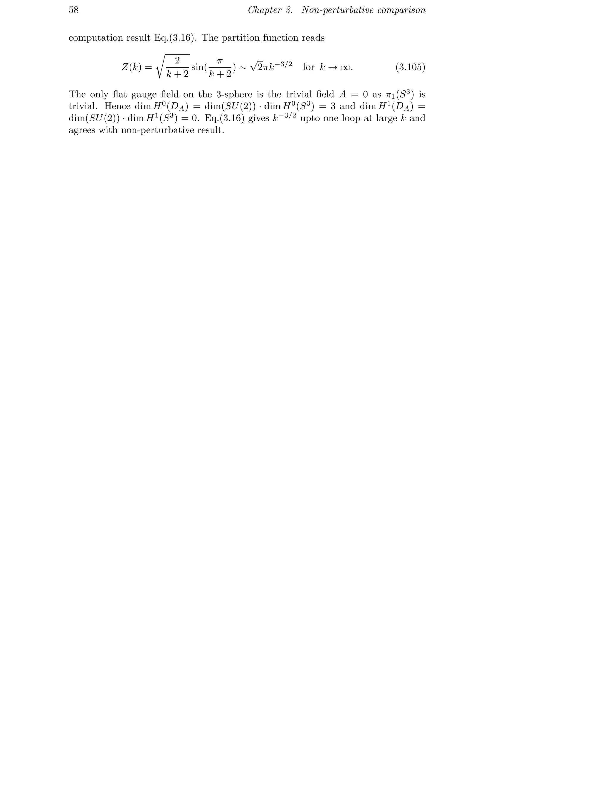
![Chapter 4
Epilogue
道可道,非常道。
—老子(Laozi), Tao Te Ching
Laozi, probably the first Chinese theoretical physicist, had ended the realm
by stating that the law of nature which can be found by people is not the never
changing law. He surely led Chinese nature science into a “bizarre” direction whilst
this conclusion might still be part of reasons young physicists of any generations
are brave enough to join a realm that having been said almost done by experts.
Moreover, he noticed that the law we are seeking is indeed an invariant. We are
not going to talk philosophy, but one worth mentioning point is its relation to
mathematics and physics. They all seem to describe some aspects of nature whilst it
is the information capacity of the languages of them distinguishes their tremendous
differences in reasoning. Mathematics as a more rigorous language compared to
speaking language makes it better tool of talking nature whilst such rigorousness
also makes it harder to translate into concrete understanding in real life. We surely
desire such understandings as they are not only providing profound comprehensions
of nature, the best things are predictions of unknowns or future. This is where
physics enters.
The interplay of mathematics and physics has been heavy once they were born.
However the fundamental problems of them diverged awhile. Their remarriage
started with use of differential geometry in relativity theory during the beginning of
20-th century, and with use of low-dimensional topology in quantum theory during
late 70s. Such trend on the one side has brought us grand new perspectives about
the world, on the other forces physicists rethinking the tool we have been used for
centuries. Until recent years people can speculate rigorous clues for axiomatically
construction of quantum mechanics[26], which categories physical world as “part”
of mathematical reality. One might be scared by leaving in the Platonic reality
59](https://image.slidesharecdn.com/96310c1d-2d9c-47cc-b2b3-bc64b84ba972-160405111747/75/Thesis-69-2048.jpg)
![60 Chapter 4. Epilogue
whilst the true “bizarreness” one needs to take care are other “parts” that different
from ours.
We see that both philosophy and mathematics would imply there are different
representations of reality. In this thesis we have seen the power of duality which
might be appropriate to regard as symmetry between representations of reality.
4.1 Discussion
Duality has a long history in mathematics, first an also simple example is between
points and lines in a plane. Any two points identify a line and if regard infinity as a
point then any two lines also identify a point, in this case we have perfect symmet-
ric descriptions of point and line in projective plane. One should also remember
vector spaces and their dual spaces in linear algebra. Direct generalization to linear
analysis, Fourier theory signals similar kind duality. In chapter 3, we have seen that
by using Poisson summation formula with which duality in Fourier theory gives the
modular invariance of theta function. We will now discussion what we have done
in each chapter and the use of duality in them.
In chapter 1 we introduced briefly about supersymmetry which can be regarded
as a duality between even and odd operators. Supersymmetry arose as the only
consistent combination of internal and Poincar´e symmetries from physics, and its
relation to differential forms seems suggest it is also mathematically elegant. More-
over with the Morse theory we can better bound the number of ground states from
perturbation theory. This is done by instaton calculation. The true ground states
are isomorphic to the cohomology of Witten complex, and it is indeed the Hodge-
de Rham cohomology. Moreover, during the instaton calculation we have seen how
would localization principle help the path integral of supersymmetric action. Indeed
localization is one elegant technic when dealing with supersymmetric perturbation
theories and it has a profound origin from topology. One direct generalization of
the Witten-Morse homology is the Floer homology where the Morse function is
given by the CS functional of su(2)-valued connection 1-forms on oriented smooth
3-manifolds. One key observation of Floer is that the gradient flows of CS are the
anti-self-duality equation for 4-manifolds, and the solutions are exactly the minima
of the Yang-Mills functional, Donaldson theory. Moreover, with knots and links
embedded Floer instanton homology is related to Khovanov homology which origi-
nally arose as a categorification of the Jones polynomial which can be obtained from
CS partition function. This leads to quantization and categorification[20, 21]. In-
stead going into such wonderful direction, we started the evaluation of CS partition
function.
In chapter 2 we started with first loop correction of perturbative CS theory. We
have seen that the Hodge duality plays the central role during the evaluation. With
standard elliptic theory we also made comments on the De Rham cohomology of
flat connection which will be important for dealing with the Floer theory. After
gauge fixing the action is topological by BRST argument. This topological model](https://image.slidesharecdn.com/96310c1d-2d9c-47cc-b2b3-bc64b84ba972-160405111747/75/Thesis-70-2048.jpg)
![4.2. Outlook 61
is a simple example of BRST formulation of topological quantum field theory. The
leading order contribution in perturbation is the Ray-Singer torsion which is a
topological invariant. With APS theorem one can fix the metric dependent phase
term to zero by adding a gravitational CS term, a local counterterm, and by the
canonical 2-framing. Therefore we arrived that the leading order contribution is
topological. For higher loop, it is always possible to add such local counterterms to
cancel out metric dependence[5, 6]. One very interesting point we did not get into
is the relation between surgery of 3-manifold and framing dependence. In topology
theories, one can usually simplify calculations by knowing how the surgery works,
and we used this simple technic to computer the exact result of CS partition function
in chapter 3. If we include knots or links in S3
, framing dependence is just about
the surgery along them. On can find more details about surgery of CS in [17]. This
can be done by adding non-trivial Wilson loops and the partition function will give
topological invariants of those loops, or knot invariants. Thus one can regard CS
partition function as generator of knots.
In chapter 3 we used affine Lie algebra to derive the exact result of CS theory,
or say the non-perturbative comparison. Started with classification of semi-simple
groups we showed that how one can characterize groups with their maximum torus,
which is the maximum Abelian subgroup. If we recall that the Green function on
torus is related to one of the Jacobi theta functions, then it would be not surprised
that we arrived a character formula with modular invariance. The generators of
this special symmetry forms PSL(2, Z) group which can be interpreted as surgery
operations on 3-manifolds. A simple example is presented to illustrate how one
uses the surgery to compute the surgery matrix. Then we showed that such surgery
matrix can help to arrive the exact result of CS. At large k limit they agree with each
other. This fact is astonishing even at first sight. It is first example of AdS3/CFT2
correspondence, and we added more details in Appendix G about this. This “new”
duality has gotten great attention. To our case, on the one side quantization of
CS leads to 2-dimensional sigma model with conformal symmetry, on the other
the coefficient of operator product expansion can be obtained by the surgery of
3-manifolds.
4.2 Outlook
Along the main stream of frontier of theoretical physics, future research of the
author will probably be focused on mathematical physics in relation with low-
dimensional topology and quantum mechanics. On the side of mathematics, we
will continue the study of interplay of Morse theory and knot theory as the fact
that the Morse theory is so effective in gaining topological information of mani-
fold from functions on it and since knots are non-trivial 1-dimensional structures
that signal a great deal of differences between dimensionality of 2 and 3. From the
physics side, relativistic extension of the Floer theory to 4-dimensional spacetime
leads one to TQFT. Moreover, the gradient flow on the space of complex-valued](https://image.slidesharecdn.com/96310c1d-2d9c-47cc-b2b3-bc64b84ba972-160405111747/75/Thesis-71-2048.jpg)
![Appendix A
Suppersymmetric non-linear
sigma model
Here we give detail relations between canonical quantisation of supersymmetric
non-linear sigma model and exterior algebra by following Witten[37]. The idea was
when we try to count the number of zero-energy states of the model whose action
is given by
L =
1
2
d2
xγij ∂µφi
∂µ
φj
+ i ¯ψi
γµ
Dµψj
+
1
4
Rijkl
¯ψi
ψk ¯ψj
ψl
, (A.1)
where γij and Rijkl are metric and curvature tensors on manifold M, and Dµ is a
covariant derivative whose action on spinor fields is given by
Dµψi
= ∂µψi
+ Γi
jk∂µφj
ψk
. (A.2)
The classical vacuum states of the theory are degenerate, thus we turn on a
perturbation that lifts the degeneracy. That is to add a generic function h(φi
),
as a “magnetic field”, define on M to the action. The new components to the
Lagrangian is
∆L = −
1
2
d2
xγij ∂h
∂φi
∂h
∂φj
+
∂2
h
∂φi∂φj
¯ψi
ψj
. (A.3)
The potential energy V (φi
) lifts the degeneracy that the energy is zero only if
∂h/∂φi
= 0.
On the other hand, since classically non-zero momentum modes carry non-zero
energies, we can determine the spectrum of low-lying states by quantizing the zero-
momentum modes. Therefore we drop the spatial dependence of φi
and ψi
and
63](https://image.slidesharecdn.com/96310c1d-2d9c-47cc-b2b3-bc64b84ba972-160405111747/75/Thesis-73-2048.jpg)
![64 Appendix A. Suppersymmetric non-linear sigma model
integrate out spatial components. Choosing a convenient base γ0
= diag(1, −1)
and consider Majorana fermion ¯ψ = (ψ†
, ψ) the simplified Lagrangian is written as
L =
1
2
L dτγij
dφi
dτ
dφj
dτ
+ iψ†i Dψj
Dτ
− i
Dψ†i
Dτ
ψj
+ Rijklψ†i
ψk
ψ†j
ψl
, (A.4)
where L is the spatial part. Under the supersymmetry transformations
δφi
= ǫψ†i
− ¯ǫψi
δψi
= ǫ(i ˙φi
− Γi
jkψ†j
ψk
)
δψ†i
= ¯ǫ(−i ˙φi
− Γi
jkψ†j
ψk
),
(A.5)
the action is invariant. By the Noether procedure, we find the corresponding su-
percharges
Q = iγijψ†i ˙φj
¯Q = −igijψi ˙φj
.
(A.6)
The conjugate momentum of φi
and ψi
are given by
pi = γij
˙φj
πψ,i = iγijψ†j
.
(A.7)
The canonical commutation and anticommutation relations are
[φi
, pj] = iδi
j
{ψi
, ψ†j
} = γij
,
(A.8)
and other relations vanish. The supercharges can be rewritten in terms of the
conjugate momentum as
Q = iψ†i
pi
Q†
= −iψi
pi.
(A.9)
Thus we see that by choosing the space of differential forms as representation
of above algebra we recover Eq.(1.1)-Eq.(1.4).
Moreover, the Lagrangian (A.4) is also invariant under the phase rotation of the
fermionic fields
ψi
→ e−iα
ψi
, ψ†i
→ eiα
ψ†i
. (A.10)
The corresponding Noether charge is given by
F = γijψ†i
ψ†i
, (A.11)
the fermion number operator. Notice that
[F, Q] = Q, [F, Q†
] = −Q†
, (A.12)
thus within the differential form representation, harmonic q-form is considered as
a state with q fermions and F in the Witten index (−1)F
is the same as fermion
number q.](https://image.slidesharecdn.com/96310c1d-2d9c-47cc-b2b3-bc64b84ba972-160405111747/75/Thesis-74-2048.jpg)


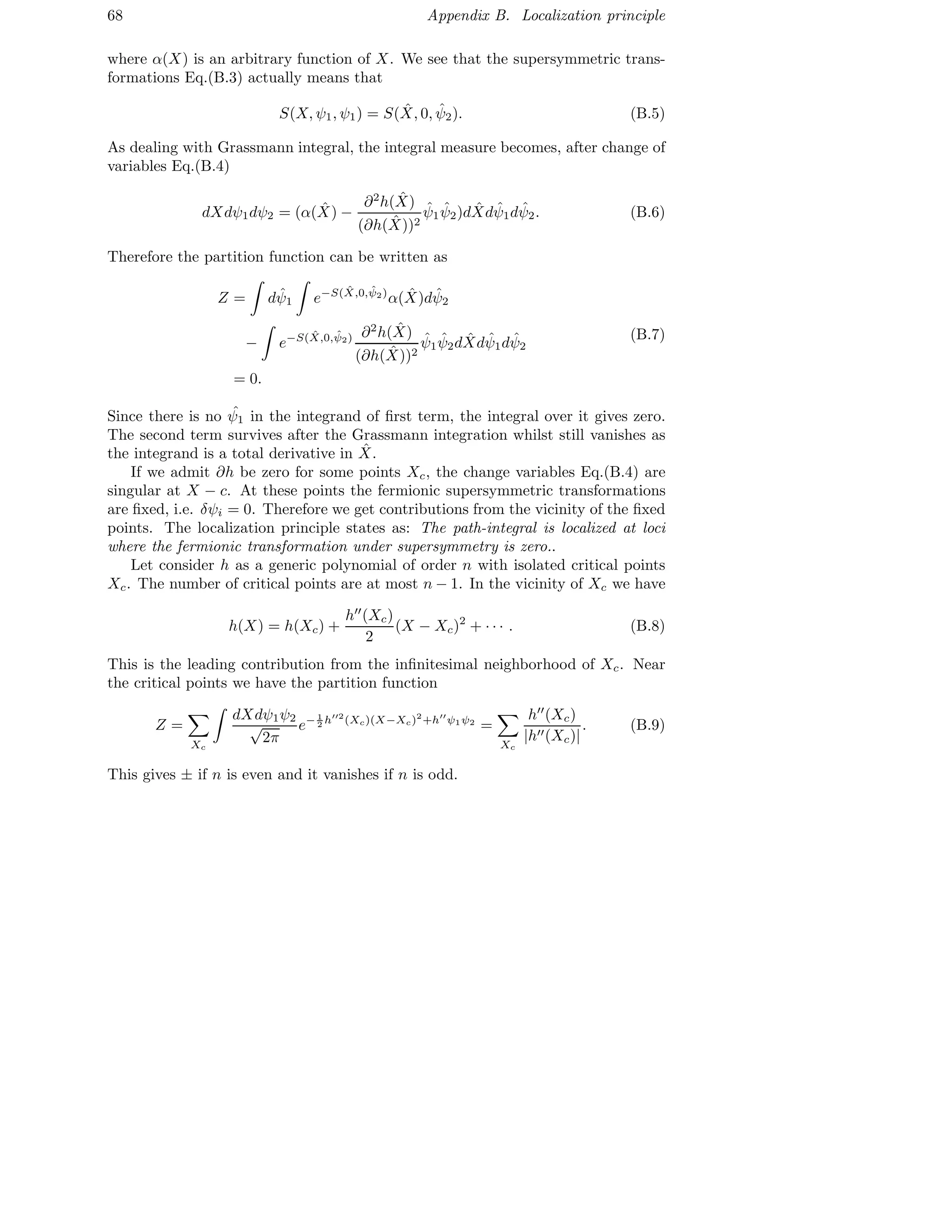
![Appendix C
Ray-Singer torsion
Here we will introduce Ray-Singer invariant, and derive the analytic torsion appears
in 1-loop correction result.
Let M be a n-dimensional compact oriented Riemannian manifold, and let K
be a simplicial complex which is a smooth triangulation of M. The Reidemeister-
Franz torsion τ of K is a function of certain representations of the fundamental
group of K. The combinatorial invariance and the equivalence of smooth trian-
gulations of M make this torsion a manifold invariant. By following Milnor[28],
give a n-dimensional vector space V over real numbers, one can have two bases
v = (v1, . . . , vn) and w = (w1, . . . , wn), and use [w/v] to denote |determinant T |,
where T represents the transformation of bases: v = T w. If [w/v] = 0 then we
can say w is equivalent to v. This will give an equivalence relation to free modules.
Now consider an exact sequence
0 → E → F → G → 0 (C.1)
of free modules. Given bases of E and G, one can construct a basis for F as
eg = (e1, · · · , ei, g′
i, · · · , g′
l), where ei ∈ E and g′
i ∈ F is lifted from gi ∈ G. We can
see the obvious dependence of eg on the choice of g′
i, whilst the equivalent class of
eg only depends on e and g. If we choose different bases ˜e and ˜g for modules E
and G, then
[˜e˜g/eg] = [˜e/e][˜g/g]. (C.2)
If we have inclusions of free modules, eg. F0 ⊂ F1 ⊂ F2 ⊂ F3, then using the exact
sequence of free quotient modules
0 → F1/F0 → F3/F0 → F2/F1 → F3/F1 → F3/F2 → 0 (C.3)
the bases bi of Fi/Fi−1 form a basis b1b2 · · · bk for Fk/F0
69](https://image.slidesharecdn.com/96310c1d-2d9c-47cc-b2b3-bc64b84ba972-160405111747/75/Thesis-79-2048.jpg)
![70 Appendix C. Ray-Singer torsion
Now we can proceed to the definition of torsion of a complex chain. Given a
chain complex
Cn → Cn−1 → · · · C1 → C0 (C.4)
of free modules that each Ci has a preferred basis ci. Let Bi denotes the image of
boundary operator ∂ : Ci+1 → Ci, Zi+1 as its kernel and Hi as the i-th homology
group. Choose bases bi and hi for Bi and Hi respectively. For each Ci we have
inclusions 0 ⊂ Bi ⊂ Zi ⊂ Ci and notice that Zi/Bi
∼= Hi, Ci/Zi
∼= Bi−1. This
suggests that by combining bases bi, hi and bi−1 we can construct a new basis
bihibi−1 for Ci. We define τ(C) = (−1)i
log[bihibi−1/ci] as the torsion of this
complex chain. The independence of τ(C) on the choice of basis bi is easily seen
by choosing a different basis ˜bi, the torsion now is written as
τ(C) = (−1)i
log[˜bihi
˜bi−1/ci]
= (−1)i
log([bihibi−1/ci][˜bi/bi][˜bi−1/bi−1])
where the last two terms sum up to zero.
To make such abstractness useful for physics, we can define an analytic ana-
logue of the torsion above when dealing with Riemannian manifold. In that case,
the metric induces a natural pairing, by the Hodge dual, that gives a preferred
orthonormal basis for each Ci. We can use the Hodge decomposition to split each
Ci as a combination of three orthogonal parts. With the help of the Laplacian
∆ = −(∂†
∂ + ∂∂†
) : Ci → Ci, we can identify the three parts of any ωq ∈ Cq as its
eigenvectors
ωq = ψq + φq + hq
∆ψi
q = −∂∂†
ψi
q = λq,iψi
q , i = 1, . . . , rq
(C.5)
where we recognize ψi
q as the i-th component of the Bq. In addition we can define
the co-boundary part φq as
φj
q = −
1
λq−1,j
∂†
ψj
q−1 , j = 1, . . . , rq−1, (C.6)
such that ∂φj
q = ψj
q−1. Notice that
|φj
q|2
=
1
λ2
q−1,j
(∂†
ψj
q−1, ∂†
ψj
q−1) = −
1
λq−1,j
, (C.7)](https://image.slidesharecdn.com/96310c1d-2d9c-47cc-b2b3-bc64b84ba972-160405111747/75/Thesis-80-2048.jpg)
![71
we finally have an orthonormal basis { −λq−1φq, ψq, hq} for Cq and the torsion of
this complex chain is
τ(C) = (−1)i
log[bihibi−1/ci]
= (−1)q
log[ψq, ∂φq, h/{ −λq−1φq, ψq, hq}]
= (−1)q
log
rq−1
j=1
(λq−1,j)−1/2
.
(C.8)
Moreover, the Laplacian is diagonal in the orthonormal basis that
(det −∆q) =
rq
j=1
(−λq,j)
rq−1
j=1
(−λq−1,j). (C.9)
By taking logarithm and induction of this, we have
log
rq−1
j=1
(−λq−1,j) =
N
k=q
(−1)k−q
log(det −∆q). (C.10)
Now we have the analytic R-torsion, or Ray-Singer torsion, as
τ(C) =
1
2
N
q=0
(−1)q+1
q log(det −∆q). (C.11)
Giving a finite-dimensional chain complex C of length n over a field F.](https://image.slidesharecdn.com/96310c1d-2d9c-47cc-b2b3-bc64b84ba972-160405111747/75/Thesis-81-2048.jpg)

![Appendix D
Gravitational Chern-Simons
People spent a lot time to formulate a gauge theory for gravity. Indeed, in 3-
dimension we have one. Such profound connection between 2 + 1-gravity and the
CS gauge theory is first noticed by Witten[39]. This is also one of the main reasons
we are interested in the pure CS theory. Concisely speaking, the Einstein-Hilbert
action of 2 + 1 dimensional manifold Y is written as
S =
1
2 Y
εijk
εabc(ea
i (∂jωbc
k − ∂kωbc
j + [ωj, ωk]bc
)). (D.1)
We can recognize the vierbein ea
i and the spin connection ωa
i b as gauge field which
is Lie-algebra valued 1-form
Ai = ea
i Pa + ωa
i Ja, Ja =
1
2
εabc
Jbc, (D.2)
where Jbc are the Lorentz generators and Pa are translations. Under this construc-
tion, Eq.(D.1) is identified with the CS invariant of ω written as
CS(ω) =
1
4π Y
Tr(ω ∧ dω +
2
3
ω ∧ ω ∧ ω). (D.3)
This is also called CS gravitational term.
73](https://image.slidesharecdn.com/96310c1d-2d9c-47cc-b2b3-bc64b84ba972-160405111747/75/Thesis-83-2048.jpg)

![Appendix E
Faddeev-Popov gauge fixing
The idea of gauge symmetry dominates modern understanding of elementary parti-
cles in quantum field theories, as most importantly, it makes one theory renormal-
izable. However it leads to infinite-dimensional spaces with infinitely many local
gauge transformations. The independence of gauge conditions is therefore crucial
for both defining and studying physical quantities in gauge theories. The action is
forced to be gauge invariant for this purpose, and the resulting Lagrangian is degen-
erate. To get rid of irrelevant degrees of freedom, here we introduce the standard
Faddeev-Popov procedure[15].
Naively, one puts a delta function δ(F(A)) in partition function as
Z = DAG (A)δ(F(A)), (E.1)
where G (A) is gauge invariant functional. However this is a bad idea that we are
dealing with non-Abelian gauge theories, and the gauge fixing function must be
local, i.e. δ(F(Agα (x))), gα means group elements parametrized by ξa
α, a is group
index. The delta function makes the integral intersecting each orbits only once, and
at the crossing point one has the local gauge fixing condition g = gα, which is non-
gauge-invariant. Unfortunately, such delta function will ruin the gauge-invariant
feature, and it gives a result that the volume of the gauge group been divided.
To solve the problem, Faddeev, Popov and De Witt found that one just need to
multiply the volume of the gauge group back by writing
V (G)/V (G) = 1 = Dgδ(g − gα), (E.2)
and the partition function now reads
Z = DADgG (A)δ(F(Agα )) det
δF(Agα )
δgβ
, (E.3)
75](https://image.slidesharecdn.com/96310c1d-2d9c-47cc-b2b3-bc64b84ba972-160405111747/75/Thesis-85-2048.jpg)
![76 Appendix E. Faddeev-Popov gauge fixing
where the determinant is Jacobian from δ(g−gα) to δ(F(Agα )). Under infinitesimal
gauge transformation, first order, gα
Agα = A + ∂ξa
αta + [A, ξα] = A + DAξα, (E.4)
where DA is the covariant exterior derivative respect to connection A and ta are
group generators, i.e. the Lie algebra of G. Therefore if F(Agα ) is linear in Agα ,
and we evaluate the determinant at identity, i.e ξa
α = 0,
det
δF(Agα )
δgβ gβ =0
= det
δF(Aα)
δAgα
δAgα
δξβ
δαβ
ξa
β=0
(E.5)
is independent of Aα, thus gauge invariant. The assumption that the measure DA
and G (A) are gauge invariant makes sure that the partition function
Z = DADgG (A)δ(F(Agα )) det
δF(Agα )
δgβ
= DAgα DgG (Agα )δ(F(Agα )) det
δF(Agα )
δgβ
= DA′
DgG (A′
)δ(F(A′
)) det
δF(Ah)
δh
= Dg DAG (A)δ(F(A)) det
δF(Ah)
δh
= V (G) DAG (A)δ(F(A)) det
δF(Ah)
δh
(E.6)
is gauge independent, we have changed the dummy variable g to h in the determi-
nant. This is the case for irreducible connection A. We will see the reducible case
in the CS theory fist noted by Rozansky[31].](https://image.slidesharecdn.com/96310c1d-2d9c-47cc-b2b3-bc64b84ba972-160405111747/75/Thesis-86-2048.jpg)
![Appendix F
BRST symmetry and gauge
fixed Chern-Simons
Following [7], we first define the BRST operator Q, which is odd derivation of the
algebra of local functionals, by its action on B, φ, C and ¯C
QBi = −(DA(α)
i + adBi)C,
Qφ = 0,
Q ¯C = φ,
QC =
1
2
[C, C] =
1
2
tafa
bccb
cc
,
(F.1)
where (adBi)c ≡ [Bi, c], and fa
bc is the structure constant of G, [tb, tc] = fa
bcta.
Acting Q on Lgauge,
QLgauge
=
−k
4π
Tr φDA(α)
i (Di
A(α) + adBi
)C + Tr(φDA(α)
i (Di
A(α) + adBi
)C
+ ¯CDA(α)
i [Di
A(α) C + [Bi
, C], C] −
1
2
¯CDA(α)
i (Di
A(α) + adBi
)[C, C])
= 0,
(F.2)
the gauged Lagrangian is invariant under BRST transformation. We continue to
investigate how the Lgauge changes under gij
→ gij
+ δgij
. Since we are dealing
with the CS theory, which is topological, δCS(B) = 0. δL will only depends on
the gauge fixing and ghosts terms as
δLgauge-fixing =
k
4π
Tr(φDA(α)
i (
√
gδgij
Bj) −
1
2
φDA(α)
k (
√
ggijδgij
gkl
Bl)) (F.3)
77](https://image.slidesharecdn.com/96310c1d-2d9c-47cc-b2b3-bc64b84ba972-160405111747/75/Thesis-87-2048.jpg)

![Appendix G
AdS3/CFT2 correspondence
To see the relation from CS to CFT, we start with part of holomorphic quantization
of Eq.(2.4). Let Az = 1
2 (Ax − iAy) and A¯z = 1
2 (Ax + iAy), the CS action is then
given by
CS = −
ik
2π t
d2
z[Tr(Az∂0A¯z − A¯z∂0Az) + iA0F¯zz]. (G.1)
The canonical commutation relations become
[Aa
z(z, ¯z), Ab
¯ω(ω, ¯ω)] =
2π
k
δab
δ(z − ω)δ(¯z − ¯ω). (G.2)
The Hilbert space is now the space of holomorphic functionals ψ of A¯z. Meanwhile
Az can be identified as the functional derivative
Aa
zψ =
2π
k
δ
δAa
¯z
ψ. (G.3)
The physical Hilbert subspace is obtained by restriction F¯zz = 0 on wave functions
(∂¯z
δ
δA¯z
+ [A¯z,
δ
δA¯z
])ψ =
k
2π
∂zA¯zψ. (G.4)
The solutions to above equation can be obtained from conformal field theory,
the WZW model. Let define map g : Σ → G with two dimensional Riemann
surface Σ and compact Lie group G. For our case we choose the group as SU(2).
The WZW action is given by
SWZW = −
1
8π Σ
d2
x
√
γγij
Tr(g−1
∂igg−1
∂jg) + iΓ(g), (G.5)
79](https://image.slidesharecdn.com/96310c1d-2d9c-47cc-b2b3-bc64b84ba972-160405111747/75/Thesis-89-2048.jpg)

![Bibliography
[1] M. Atiyah. New invariants of 3-and 4-dimensional manifolds. The mathematical
heritage of Hermann Weyl (Durham, NC, 1987), 48:285–299, 1988.
[2] M. Atiyah. On framings of 3-manifolds. Topology, 29(1):1–7, 1990.
[3] M. Atiyah, R. Bott, and V.K. Patodi. On the heat equation and the index
theorem. Inventiones mathematicæ, 19(4):279–330, 1973.
[4] M. Atiyah, V.K. Patodi, and I.M. Singer. Spectral asymmetry and riemannian
geometry. ii. In Math. Proc. Camb. Phil. Soc, volume 78, pages 405–432.
Cambridge Univ Press, 1975.
[5] S. Axelrod and I.M. Singer. Chern-simons perturbation theory. 1991.
[6] S. Axelrod and I.M. Singer. Chern–simons perturbation theory ii. arXiv
preprint hep-th/9304087, 1993.
[7] D. Bar-Natan. Perturbative chern-simons theory. Journal of Knot Theory and
its Ramifications, 4(04):503–547, 1995.
[8] C. Becchi, A. Rouet, and R. Stora. Renormalization of the abelian higgs-kibble
model. Communications in Mathematical Physics, 42(2):127–162, 1975.
[9] J.M. Bismut and D.S. Freed. The analysis of elliptic families: Ii. dirac oper-
ators, eta invariants, and the holonomy theorem. Communications in Mathe-
matical Physics, 107:103–163, 1986.
[10] T. Br¨ocker and T.T. Dieck. Representations of compact Lie groups, volume 98.
Springer, 1985.
[11] S.K. Donaldson. An application of gauge theory to four dimensional topology.
Journal of Differential Geometry, 18(2):279–315, 1983.
[12] S.K. Donaldson. The orientation ofyang-mills moduli spaces and 4-manifold
topology. J. Diff. Geo, 26:397–428, 1987.
81](https://image.slidesharecdn.com/96310c1d-2d9c-47cc-b2b3-bc64b84ba972-160405111747/75/Thesis-91-2048.jpg)
![82 Bibliography
[13] S.K. Donaldson. Polynomial invariants for smooth four-manifolds. Topology,
29(3):257–315, 1990.
[14] S. Elitzur, G. Moore, A. Schwimmer, and N. Seiberg. Remarks on the canonical
quantization of the chern-simons-witten theory. Nuclear Physics B, 326(1):108–
134, 1989.
[15] L.D. Faddeev and V.N. Popov. Feynman diagrams for the yang-mills field.
Physics Letters B, 25(1):29–30, 1967.
[16] A. Floer. An instanton-invariant for 3-manifolds. Communications in mathe-
matical physics, 118(2):215–240, 1988.
[17] D.S. Freed and R.E. Gompf. Computer calculation of witten’s 3-manifold
invariant. Communications in mathematical physics, 141(1):79–117, 1991.
[18] E. Frenkel and E. Witten. Geometric endoscopy and mirror symmetry. arXiv
preprint arXiv:0710.5939, 2007.
[19] D. Gepner and E. Witten. String theory on group manifolds. Nuclear Physics
B, 278(3):493–549, 1986.
[20] S. Gukov. Three-dimensional quantum gravity, chern-simons theory, and the
a polynomial. Commun.Math.Phys., 255:577–627, 2005.
[21] S. Gukov and P. Sulkowski. A-polynomial, b-model, and quantization. Journal
of High Energy Physics, 2012(2):1–57, 2012.
[22] S. Gukov and E. Witten. Gauge theory, ramification, and the geometric lang-
lands program. arXiv preprint hep-th/0612073, 2006.
[23] K. Hori. Mirror symmetry, volume 1. American Mathematical Soc., 2003.
[24] V.G. Kac. Infinite-dimensional Lie algebras, volume 44. Cambridge University
Press, 1994.
[25] V.G. Kac and D.H. Peterson. Infinite-dimensional lie algebras, theta functions
and modular forms. 1984.
[26] A. Kapustin. Is there life beyond quantum mechanics? 2013.
[27] A. Kapustin and E. Witten. Electric-magnetic duality and the geometric lang-
lands program. arXiv preprint hep-th/0604151, 2006.
[28] J. Milnor. Whitehead torsion. Bulletin (New Series) of the American Mathe-
matical Society, 72(3):358–426, 1966.
[29] J. Qiu. Lecture notes on topological field theory: Perturbative and non-
perturbative aspects. 2012.](https://image.slidesharecdn.com/96310c1d-2d9c-47cc-b2b3-bc64b84ba972-160405111747/75/Thesis-92-2048.jpg)
![Bibliography 83
[30] D.B. Ray and I.M. Singer. R torsion and the laplacian on riemannian mani-
folds. Adv.Math., 7:145–210, 1971.
[31] L. Rozansky. A large k asymptotics of witten’s invariant of seifert manifolds.
Communications in Mathematical Physics, 171(2):279–322, 1995.
[32] A.S. Schwarz. The partition function of degenerate quadratic functional and
ray-singer invariants. Letters in Mathematical Physics, 2(3):247–252, 1978.
[33] S. Axelrod S.D. Pietra and E. Witten. Geometric quantization of chern-simons
gauge theory. 1991.
[34] C.H. Taubes. A framework for morse theory for the yang-mills functional.
Inventiones mathematicae, 94(2):327–402, 1988.
[35] I.V. Tyutin. Lebedev institute preprint. N39, 1975.
[36] E. Verlinde. Fusion rules and modular transformations in 2d conformal field
theory. Nuclear Physics B, 300:360–376, 1988.
[37] E. Witten. Constraints on supersymmetry breaking. Nuclear Physics B,
202(2):253–316, 1982.
[38] E. Witten. Supersymmetry and morse theory. Journal of Differential Geome-
try, 17(4):661–692, 1982.
[39] E. Witten. 2+ 1 dimensional gravity as an exactly soluble system. Nuclear
Physics B, 311(1):46–78, 1988.
[40] E. Witten. Topological quantum field theory. Communications in Mathemat-
ical Physics, 117(3):353–386, 1988.
[41] E. Witten. Gauge theories and integrable lattice models. Nuclear Physics B,
322(3):629–697, 1989.
[42] E. Witten. Quantum field theory and the jones polynomial. Communications
in Mathematical Physics, 121:351–399, September 1989.
[43] E. Witten. Gauge theories, vertex models, and quantum groups. Nuclear
Physics B, 330(2):285–346, 1990.](https://image.slidesharecdn.com/96310c1d-2d9c-47cc-b2b3-bc64b84ba972-160405111747/75/Thesis-93-2048.jpg)


