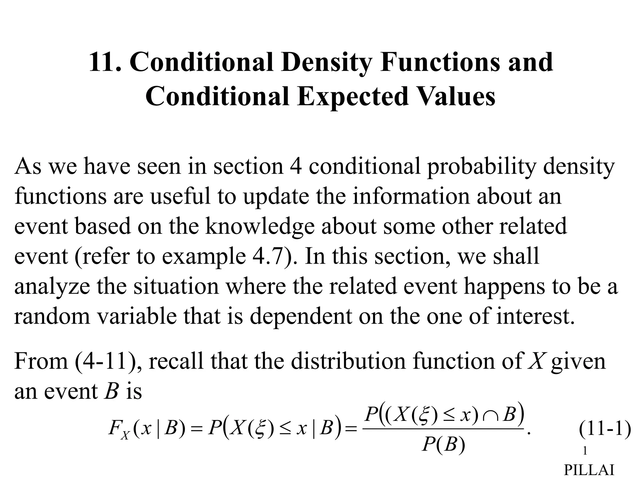
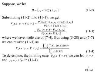
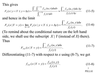
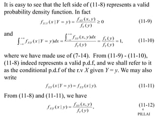
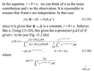
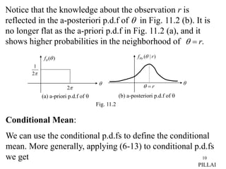
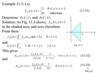
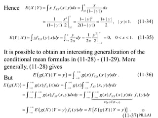
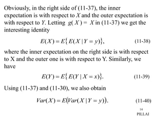
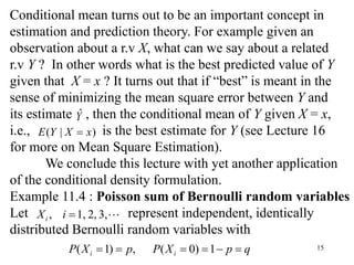
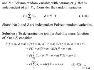
The document discusses conditional probability density functions and conditional expected values. It defines the conditional probability density function of a random variable X given another random variable Y=y as f(x|y). This allows updating knowledge about X based on information about Y. The conditional expected value of X given Y=y is defined as the integral of xf(x|y)dx. An example calculates the conditional PDFs and expected value for two random variables with a given joint PDF.

1. 1
As we have seen in section 4 conditional probability density
functions are useful to update the information about an
event based on the knowledge about some other related
event (refer to example 4.7). In this section, we shall
analyze the situation where the related event happens to be a
random variable that is dependent on the one of interest.
From (4-11), recall that the distribution function of X given
an event B is
(11-1)
   .
)
(
)
)
(
(
|
)
(
)
|
(
B
P
B
x
X
P
B
x
X
P
B
x
FX







PILLAI
11. Conditional Density Functions and
Conditional Expected Values

2. 2
Suppose, we let
Substituting (11-2) into (11-1), we get
where we have made use of (7-4). But using (3-28) and (7-7)
we can rewrite (11-3) as
To determine, the limiting case we can let
and in (11-4).
 .
)
( 2
1 y
Y
y
B 

 
(11-3)
(11-2)
 
,
)
(
)
(
)
,
(
)
,
(
)
)
(
(
)
(
,
)
(
)
|
(
1
2
1
2
2
1
2
1
2
1
y
F
y
F
y
x
F
y
x
F
y
Y
y
P
y
Y
y
x
X
P
y
Y
y
x
F
Y
Y
XY
XY
X














.
)
(
)
,
(
)
|
( 2
1
2
1
2
1

 




 y
y
Y
x y
y
XY
X
dv
v
f
dudv
v
u
f
y
Y
y
x
F
(11-4)
),
|
( y
Y
x
FX  y
y 
1
y
y
y 


2
PILLAI

3. 3
This gives
and hence in the limit
(To remind about the conditional nature on the left hand
side, we shall use the subscript X | Y (instead of X) there).
Thus
Differentiating (11-7) with respect to x using (8-7), we get
(11-5)
(11-6)
.
)
(
)
,
(
)
|
(
lim
)
|
(
0 y
f
du
y
u
f
y
y
Y
y
x
F
y
Y
x
F
Y
x
XY
X
y
X
 










(11-7)
(11-8)
y
y
f
y
du
y
u
f
dv
v
f
dudv
v
u
f
y
y
Y
y
x
F
Y
x
XY
y
y
y
Y
x y
y
y
XY
X










  







)
(
)
,
(
)
(
)
,
(
)
|
(
.
)
(
)
,
(
)
|
(
|
y
f
du
y
u
f
y
Y
x
F
Y
x
XY
Y
X
 



.
)
(
)
,
(
)
|
(
|
y
f
y
x
f
y
Y
x
f
Y
XY
Y
X 

PILLAI

4. 4
It is easy to see that the left side of (11-8) represents a valid
probability density function. In fact
and
where we have made use of (7-14). From (11-9) - (11-10),
(11-8) indeed represents a valid p.d.f, and we shall refer to it
as the conditional p.d.f of the r.v X given Y = y. We may also
write
From (11-8) and (11-11), we have
(11-9)
|
( , )
( | ) 0
( )
XY
X Y
Y
f x y
f x Y y
f y
  
,
1
)
(
)
(
)
(
)
,
(
)
|
(
| 












 y
f
y
f
y
f
dx
y
x
f
dx
y
Y
x
f
Y
Y
Y
XY
Y
X
(11-10)
(11-11)
,
)
(
)
,
(
)
|
(
|
y
f
y
x
f
y
x
f
Y
XY
Y
X  (11-12)
PILLAI
).
|
(
)
|
( |
| y
x
f
y
Y
x
f Y
X
Y
X 


5. 5
and similarly
If the r.vs X and Y are independent, then
and (11-12) - (11-13) reduces to
implying that the conditional p.d.fs coincide with their
unconditional p.d.fs. This makes sense, since if X and Y are
independent r.vs, information about Y shouldn’t be of any
help in updating our knowledge about X.
In the case of discrete-type r.vs, (11-12) reduces to
)
(
)
(
)
,
( y
f
x
f
y
x
f Y
X
XY 
(11-13)
(11-14)
(11-15)
.
)
(
)
,
(
)
|
(
|
x
f
y
x
f
x
y
f
X
XY
X
Y 
),
(
)
|
(
),
(
)
|
( |
| y
f
x
y
f
x
f
y
x
f Y
X
Y
X
Y
X 

  .
)
(
)
,
(
|
j
j
i
j
i
y
Y
P
y
Y
x
X
P
y
Y
x
X
P






PILLAI

6. 6
Next we shall illustrate the method of obtaining conditional
p.d.fs through an example.
Example 11.1: Given
determine and
Solution: The joint p.d.f is given to be a constant in the
shaded region. This gives
Similarly
and
(11-16)


 



,
otherwise
,
0
,
1
0
,
)
,
(
y
x
k
y
x
fXY
.
2
1
2
)
,
(
1
0
1
0 0





 
   k
k
dy
y
k
dy
dx
k
dxdy
y
x
f
y
XY
)
|
(
| y
x
f Y
X ).
|
(
| x
y
f X
Y
x
y
1
1
Fig. 11.1
,
1
0
),
1
(
)
,
(
)
(
1





 
 x
x
k
dy
k
dy
y
x
f
x
f
x
XY
X
(11-17)
.
1
0
,
)
,
(
)
(
0




 
 y
y
k
dx
k
dx
y
x
f
y
f
y
XY
Y
(11-18)
PILLAI

7. 7
From (11-16) - (11-18), we get
and
We can use (11-12) - (11-13) to derive an important result.
From there, we also have
or
But
and using (11-23) in (11-22), we get
(11-19)
(11-20)
(11-21)
,
1
0
,
1
)
(
)
,
(
)
|
(
| 



 y
x
y
y
f
y
x
f
y
x
f
Y
XY
Y
X
.
1
0
,
1
1
)
(
)
,
(
)
|
(
| 




 y
x
x
x
f
y
x
f
x
y
f
X
XY
X
Y
)
(
)
|
(
)
(
)
|
(
)
,
( |
| x
f
x
y
f
y
f
y
x
f
y
x
f X
X
Y
Y
Y
X
XY 

.
)
(
)
(
)
|
(
)
|
( |
|
x
f
y
f
y
x
f
x
y
f
X
Y
Y
X
X
Y  (11-22)











 | )
(
)
|
(
)
,
(
)
( dy
y
f
y
x
f
dy
y
x
f
x
f Y
Y
X
XY
X (11-23)
PILLAI

8. 8
Equation (11-24) represents the p.d.f version of Bayes’
theorem. To appreciate the full significance of (11-24), one
need to look at communication problems where
observations can be used to update our knowledge about
unknown parameters. We shall illustrate this using a simple
example.
Example 11.2: An unknown random phase  is uniformly
distributed in the interval and where
n  Determine
Solution: Initially almost nothing about the r.v  is known,
so that we assume its a-priori p.d.f to be uniform in the
interval
.
)
(
)
|
(
)
(
)
|
(
)
|
(
|
|






dy
y
f
y
x
f
y
f
y
x
f
x
y
f
Y
Y
X
Y
Y
X
YX (24)
),
2
,
0
(  ,
n
r 

).
,
0
( 2

N ).
|
( r
f 
).
2
,
0
( 
PILLAI

9. 9
In the equation we can think of n as the noise
contribution and r as the observation. It is reasonable to
assume that  and n are independent. In that case

since it is given that is a constant, behaves
like n. Using (11-24), this gives the a-posteriori p.d.f of 
given r to be (see Fig. 11.2 (b))
where
,
n
r 

)
,
(
)
|
( 2


 N
r
f 
θ (11-25)


θ
,
2
0
,
)
(
2
1
)
(
)
|
(
)
(
)
|
(
)
|
(
2
2
2
2
2
2
2
/
)
(
2
0
2
/
)
(
2
/
)
(
2
0


































r
r
r
e
r
d
e
e
d
f
r
f
f
r
f
r
f
.
2
)
( 2
0
2
/
)
( 2
2



 





d
e
r
r
(11-26)
n
r 

PILLAI

10. 10
Notice that the knowledge about the observation r is
reflected in the a-posteriori p.d.f of  in Fig. 11.2 (b). It is
no longer flat as the a-priori p.d.f in Fig. 11.2 (a), and it
shows higher probabilities in the neighborhood of .
r


)
|
(
| r
f r 


(b) a-posteriori p.d.f of 
r


Fig. 11.2
Conditional Mean:
We can use the conditional p.d.fs to define the conditional
mean. More generally, applying (6-13) to conditional p.d.fs
we get
)
(

f

(a) a-priori p.d.f of 

2
1

2
PILLAI

11. 11
 
( ) | ( ) ( | ) .
X
E g X B g x f x B dx


  (11-27)
and using a limiting argument as in (11-2) - (11-8), we get
to be the conditional mean of X given Y = y. Notice
that will be a function of y. Also
In a similar manner, the conditional variance of X given Y
= y is given by
we shall illustrate these calculations through an example.
  






 |
| )
|
(
| dx
y
x
f
x
y
Y
X
E Y
X
Y
X
 (11-28)
)
|
( y
Y
X
E 
  .
)
|
(
| |
| 






 dy
x
y
f
y
x
X
Y
E X
Y
X
Y
 (11-29)
   
 .
|
)
(
)
|
(
|
)
|
(
2
|
2
2
2
|
y
Y
X
E
y
Y
X
E
y
Y
X
E
Y
X
Var
Y
X
Y
X










(11-30)
PILLAI

12. 12
Example 11.3: Let
Determine and
Solution: As Fig. 11.3 shows,
in the shaded area, and zero elsewhere.
From there
and
This gives
and


 



.
otherwise
,
0
,
1
|
|
0
,
1
)
,
(
x
y
y
x
fXY (11-31)
)
|
( Y
X
E ).
|
( X
Y
E
,
1
0
,
2
)
,
(
)
( 


 
x
x
dy
y
x
f
x
f
x
x
XY
X
1
| |
( ) 1 1 | |, | | 1,
Y
y
f y dx y y
   

,
1
|
|
0
,
|
|
1
1
)
(
)
,
(
)
|
(
| 




 x
y
y
y
f
y
x
f
y
x
f
Y
XY
Y
X
.
1
|
|
0
,
2
1
)
(
)
,
(
)
|
(
| 



 x
y
x
x
f
y
x
f
x
y
f
X
XY
X
Y
(11-32)
(11-33)
x
y
1
Fig. 11.3
1
)
,
( 
y
x
fXY
PILLAI

13. 13
Hence
It is possible to obtain an interesting generalization of the
conditional mean formulas in (11-28) - (11-29). More
generally, (11-28) gives
But
.
1
|
|
,
2
|
|
1
|)
|
1
(
2
|
|
1
2
|)
|
1
(
1
|)
|
1
(
)
|
(
)
|
(
2
1
|
|
2
1
|
|
|










  
y
y
y
y
x
y
dx
y
x
dx
y
x
f
x
Y
X
E
y
y
Y
X
.
1
0
,
0
2
2
1
2
)
|
(
)
|
(
2
| 







  x
y
x
dy
x
y
dy
x
y
yf
X
Y
E
x
x
x
x
X
Y
(11-34)
(11-35)
 
 
 
|
( )|
( ) ( ) ( ) ( ) ( , )
( ) ( , ) ( ) ( | ) ( )
( ) | ( )
X XY
XY X Y Y
E g X Y y
Y
E g X g x f x dx g x f x y dydx
g x f x y dxdy g x f x y dx f y dy
E g X Y y f y dy E E
  
  
   
   



 
 
  
  
   
  
 
( ) | .
g X Y y

  |
( ) | ( ) ( | ) .
X Y
E g X Y y g x f x y dx


   (11-36)
(11-37)PILLAI

14. 14
Obviously, in the right side of (11-37), the inner
expectation is with respect to X and the outer expectation is
with respect to Y. Letting g( X ) = X in (11-37) we get the
interesting identity
where the inner expectation on the right side is with respect
to X and the outer one is with respect to Y. Similarly, we
have
Using (11-37) and (11-30), we also obtain
 ,
)
|
(
)
( y
Y
X
E
E
X
E 

 .
)
|
(
)
( x
X
Y
E
E
Y
E 

(11-38)
(11-39)
 .
)
|
(
)
( y
Y
X
Var
E
X
Var 
 (11-40)
PILLAI

15. 15
Conditional mean turns out to be an important concept in
estimation and prediction theory. For example given an
observation about a r.v X, what can we say about a related
r.v Y ? In other words what is the best predicted value of Y
given that X = x ? It turns out that if “best” is meant in the
sense of minimizing the mean square error between Y and
its estimate , then the conditional mean of Y given X = x,
i.e., is the best estimate for Y (see Lecture 16
for more on Mean Square Estimation).
We conclude this lecture with yet another application
of the conditional density formulation.
Example 11.4 : Poisson sum of Bernoulli random variables
Let represent independent, identically
distributed Bernoulli random variables with
Yˆ
)
|
( x
X
Y
E 

3,
2,
1,
, 
i
Xi
q
p
X
P
p
X
P i
i 




 1
)
0
(
,
)
1
(

16. 16
and N a Poisson random variable with parameter that is
independent of all . Consider the random variables
Show that Y and Z are independent Poisson random variables.
Solution : To determine the joint probability mass function
of Y and Z, consider
.
,
1
Y
N
Z
X
Y
N
i
i 

 

(11-41)
i
X

PILLAI































n
m
i
i
N
i
i
n
m
N
P
m
X
P
n
m
N
P
n
m
N
m
X
P
n
m
N
P
n
m
N
m
Y
P
n
m
N
m
Y
P
n
Y
N
m
Y
P
n
Z
m
Y
P
1
1
)
(
)
(
)
(
)
(
)
(
)
(
)
,
(
)
,
(
)
,
(
(11-42)

17. 17
)
)
,
(
~
( of
t
independen
are
and
that
Note
1
N
s
X
p
n
m
B
X i
n
m
i
i 



(11-43)
( )!
! ! ( )!
m n
m n
m n
p q e
m n m n
  

  
 
    

   












 

!
)
(
!
)
(
n
q
e
m
p
e
n
q
m
p 
 

).
(
)
( n
Z
P
m
Y
P 


PILLAI
Thus
and Y and Z are independent random variables.
Thus if a bird lays eggs that follow a Poisson random
variable with parameter , and if each egg survives
)
(
~
)
(
~ and 
 q
P
Z
p
P
Y (11-44)


18. 18
with probability p, then the number of chicks that survive
also forms a Poisson random variable with parameter .

p
PILLAI