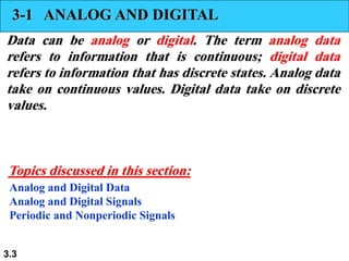
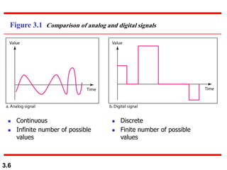
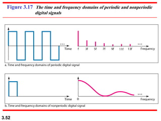
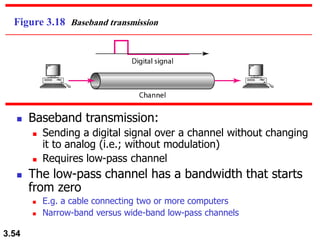
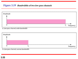
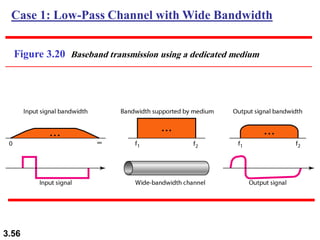
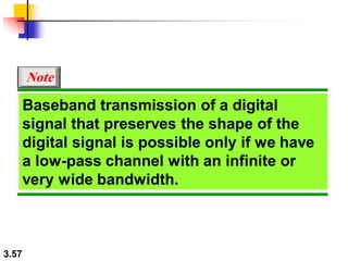
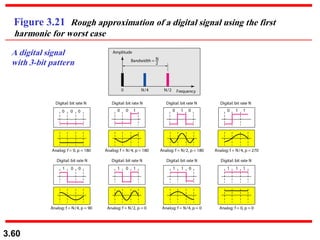
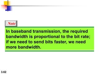
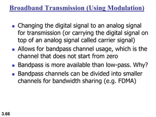
Data can exist in either analog or digital form. Analog data is continuous while digital data takes on discrete values. Signals can also be analog or digital, with analog signals having an infinite number of possible values and digital signals having a finite set of values. For data to be transmitted, it must be converted into electromagnetic signals. Baseband transmission of digital signals is only possible if the channel has an extremely wide bandwidth to preserve the shape of the digital signal.
Data and signals are fundamental concepts in the field of communication and information technology. In general, data refers to any information that can be represented in a digital format, while a signal is an analog or digital representation of data that can be transmitted over a communication channel.
There are many ways to present data and signals, and the choice depends on the specific application and requirements of the system. In this answer, we will discuss some common methods used for data and signal presentation.
Analog Signals:
Analog signals are continuous and can take any value within a certain range. Examples of analog signals include sound waves, voltage or current signals in electrical circuits, and temperature measurements. Analog signals can be presented graphically using waveform plots or oscilloscopes. The amplitude of the signal is plotted on the vertical axis, while time is plotted on the horizontal axis.
Digital Signals:
Digital signals, on the other hand, are discrete and take on only a finite set of values. These values are represented by binary digits (bits), which can take on the values of 0 or 1. Digital signals are used in many digital communication systems, such as computers, telecommunication networks, and the internet. Digital signals can be presented in several ways, such as waveform plots, histograms, and eye diagrams.
Textual Data:
Textual data refers to data that is represented by characters, such as letters, numbers, and symbols. Textual data can be presented in many ways, such as plain text, tables, spreadsheets, and databases. Textual data can also be formatted in different ways, such as font size, style, and color.
Graphical Data:
Graphical data refers to data that is presented in a graphical form, such as charts, graphs, and diagrams. Graphical data is commonly used to represent trends, patterns, and relationships between different variables. Common types of graphical data include bar charts, line graphs, scatter plots, and pie charts.
Multimedia Data:
Multimedia data refers to data that includes various types of media, such as images, videos, and audio. Multimedia data can be presented in many different formats, such as JPEG, MPEG, and WAV. Multimedia data can also be compressed and transmitted over networks using various compression techniques, such as JPEG compression and MP3 compression.
In conclusion, data and signals can be presented in many ways, depending on the specific application and requirements of the system. The choice of presentation method will depend on factors such as the type of data or signal being presented, the accuracy and resolution required, and the constraints of the communication system.
Hybrid optimization of pumped hydro system and solar- Engr. Abdul-Azeez.pdffxintegritypublishin
Advancements in technology unveil a myriad of electrical and electronic breakthroughs geared towards efficiently harnessing limited resources to meet human energy demands. The optimization of hybrid solar PV panels and pumped hydro energy supply systems plays a pivotal role in utilizing natural resources effectively. This initiative not only benefits humanity but also fosters environmental sustainability. The study investigated the design optimization of these hybrid systems, focusing on understanding solar radiation patterns, identifying geographical influences on solar radiation, formulating a mathematical model for system optimization, and determining the optimal configuration of PV panels and pumped hydro storage. Through a comparative analysis approach and eight weeks of data collection, the study addressed key research questions related to solar radiation patterns and optimal system design. The findings highlighted regions with heightened solar radiation levels, showcasing substantial potential for power generation and emphasizing the system's efficiency. Optimizing system design significantly boosted power generation, promoted renewable energy utilization, and enhanced energy storage capacity. The study underscored the benefits of optimizing hybrid solar PV panels and pumped hydro energy supply systems for sustainable energy usage. Optimizing the design of solar PV panels and pumped hydro energy supply systems as examined across diverse climatic conditions in a developing country, not only enhances power generation but also improves the integration of renewable energy sources and boosts energy storage capacities, particularly beneficial for less economically prosperous regions. Additionally, the study provides valuable insights for advancing energy research in economically viable areas. Recommendations included conducting site-specific assessments, utilizing advanced modeling tools, implementing regular maintenance protocols, and enhancing communication among system components.
NUMERICAL SIMULATIONS OF HEAT AND MASS TRANSFER IN CONDENSING HEAT EXCHANGERS...ssuser7dcef0
Power plants release a large amount of water vapor into the
atmosphere through the stack. The flue gas can be a potential
source for obtaining much needed cooling water for a power
plant. If a power plant could recover and reuse a portion of this
moisture, it could reduce its total cooling water intake
requirement. One of the most practical way to recover water
from flue gas is to use a condensing heat exchanger. The power
plant could also recover latent heat due to condensation as well
as sensible heat due to lowering the flue gas exit temperature.
Additionally, harmful acids released from the stack can be
reduced in a condensing heat exchanger by acid condensation. reduced in a condensing heat exchanger by acid condensation.
Condensation of vapors in flue gas is a complicated
phenomenon since heat and mass transfer of water vapor and
various acids simultaneously occur in the presence of noncondensable
gases such as nitrogen and oxygen. Design of a
condenser depends on the knowledge and understanding of the
heat and mass transfer processes. A computer program for
numerical simulations of water (H2O) and sulfuric acid (H2SO4)
condensation in a flue gas condensing heat exchanger was
developed using MATLAB. Governing equations based on
mass and energy balances for the system were derived to
predict variables such as flue gas exit temperature, cooling
water outlet temperature, mole fraction and condensation rates
of water and sulfuric acid vapors. The equations were solved
using an iterative solution technique with calculations of heat
and mass transfer coefficients and physical properties.
KuberTENes Birthday Bash Guadalajara - K8sGPT first impressionsVictor Morales
K8sGPT is a tool that analyzes and diagnoses Kubernetes clusters. This presentation was used to share the requirements and dependencies to deploy K8sGPT in a local environment.
Harnessing WebAssembly for Real-time Stateless Streaming PipelinesChristina Lin
Traditionally, dealing with real-time data pipelines has involved significant overhead, even for straightforward tasks like data transformation or masking. However, in this talk, we’ll venture into the dynamic realm of WebAssembly (WASM) and discover how it can revolutionize the creation of stateless streaming pipelines within a Kafka (Redpanda) broker. These pipelines are adept at managing low-latency, high-data-volume scenarios.
Saudi Arabia stands as a titan in the global energy landscape, renowned for its abundant oil and gas resources. It's the largest exporter of petroleum and holds some of the world's most significant reserves. Let's delve into the top 10 oil and gas projects shaping Saudi Arabia's energy future in 2024.
Water billing management system project report.pdfKamal Acharya
Our project entitled “Water Billing Management System” aims is to generate Water bill with all the charges and penalty. Manual system that is employed is extremely laborious and quite inadequate. It only makes the process more difficult and hard.
The aim of our project is to develop a system that is meant to partially computerize the work performed in the Water Board like generating monthly Water bill, record of consuming unit of water, store record of the customer and previous unpaid record.
We used HTML/PHP as front end and MYSQL as back end for developing our project. HTML is primarily a visual design environment. We can create a android application by designing the form and that make up the user interface. Adding android application code to the form and the objects such as buttons and text boxes on them and adding any required support code in additional modular.
MySQL is free open source database that facilitates the effective management of the databases by connecting them to the software. It is a stable ,reliable and the powerful solution with the advanced features and advantages which are as follows: Data Security.MySQL is free open source database that facilitates the effective management of the databases by connecting them to the software.
Literature Review Basics and Understanding Reference Management.pptxDr Ramhari Poudyal
Three-day training on academic research focuses on analytical tools at United Technical College, supported by the University Grant Commission, Nepal. 24-26 May 2024
Forklift Classes Overview by Intella PartsIntella Parts
Discover the different forklift classes and their specific applications. Learn how to choose the right forklift for your needs to ensure safety, efficiency, and compliance in your operations.
For more technical information, visit our website https://intellaparts.com
NO1 Uk best vashikaran specialist in delhi vashikaran baba near me online vas...Amil Baba Dawood bangali
Contact with Dawood Bhai Just call on +92322-6382012 and we'll help you. We'll solve all your problems within 12 to 24 hours and with 101% guarantee and with astrology systematic. If you want to take any personal or professional advice then also you can call us on +92322-6382012 , ONLINE LOVE PROBLEM & Other all types of Daily Life Problem's.Then CALL or WHATSAPP us on +92322-6382012 and Get all these problems solutions here by Amil Baba DAWOOD BANGALI
#vashikaranspecialist #astrologer #palmistry #amliyaat #taweez #manpasandshadi #horoscope #spiritual #lovelife #lovespell #marriagespell#aamilbabainpakistan #amilbabainkarachi #powerfullblackmagicspell #kalajadumantarspecialist #realamilbaba #AmilbabainPakistan #astrologerincanada #astrologerindubai #lovespellsmaster #kalajaduspecialist #lovespellsthatwork #aamilbabainlahore#blackmagicformarriage #aamilbaba #kalajadu #kalailam #taweez #wazifaexpert #jadumantar #vashikaranspecialist #astrologer #palmistry #amliyaat #taweez #manpasandshadi #horoscope #spiritual #lovelife #lovespell #marriagespell#aamilbabainpakistan #amilbabainkarachi #powerfullblackmagicspell #kalajadumantarspecialist #realamilbaba #AmilbabainPakistan #astrologerincanada #astrologerindubai #lovespellsmaster #kalajaduspecialist #lovespellsthatwork #aamilbabainlahore #blackmagicforlove #blackmagicformarriage #aamilbaba #kalajadu #kalailam #taweez #wazifaexpert #jadumantar #vashikaranspecialist #astrologer #palmistry #amliyaat #taweez #manpasandshadi #horoscope #spiritual #lovelife #lovespell #marriagespell#aamilbabainpakistan #amilbabainkarachi #powerfullblackmagicspell #kalajadumantarspecialist #realamilbaba #AmilbabainPakistan #astrologerincanada #astrologerindubai #lovespellsmaster #kalajaduspecialist #lovespellsthatwork #aamilbabainlahore #Amilbabainuk #amilbabainspain #amilbabaindubai #Amilbabainnorway #amilbabainkrachi #amilbabainlahore #amilbabaingujranwalan #amilbabainislamabad
An Approach to Detecting Writing Styles Based on Clustering Techniquesambekarshweta25
An Approach to Detecting Writing Styles Based on Clustering Techniques
Authors:
-Devkinandan Jagtap
-Shweta Ambekar
-Harshit Singh
-Nakul Sharma (Assistant Professor)
Institution:
VIIT Pune, India
Abstract:
This paper proposes a system to differentiate between human-generated and AI-generated texts using stylometric analysis. The system analyzes text files and classifies writing styles by employing various clustering algorithms, such as k-means, k-means++, hierarchical, and DBSCAN. The effectiveness of these algorithms is measured using silhouette scores. The system successfully identifies distinct writing styles within documents, demonstrating its potential for plagiarism detection.
Introduction:
Stylometry, the study of linguistic and structural features in texts, is used for tasks like plagiarism detection, genre separation, and author verification. This paper leverages stylometric analysis to identify different writing styles and improve plagiarism detection methods.
Methodology:
The system includes data collection, preprocessing, feature extraction, dimensional reduction, machine learning models for clustering, and performance comparison using silhouette scores. Feature extraction focuses on lexical features, vocabulary richness, and readability scores. The study uses a small dataset of texts from various authors and employs algorithms like k-means, k-means++, hierarchical clustering, and DBSCAN for clustering.
Results:
Experiments show that the system effectively identifies writing styles, with silhouette scores indicating reasonable to strong clustering when k=2. As the number of clusters increases, the silhouette scores decrease, indicating a drop in accuracy. K-means and k-means++ perform similarly, while hierarchical clustering is less optimized.
Conclusion and Future Work:
The system works well for distinguishing writing styles with two clusters but becomes less accurate as the number of clusters increases. Future research could focus on adding more parameters and optimizing the methodology to improve accuracy with higher cluster values. This system can enhance existing plagiarism detection tools, especially in academic settings.
Hierarchical Digital Twin of a Naval Power SystemKerry Sado
A hierarchical digital twin of a Naval DC power system has been developed and experimentally verified. Similar to other state-of-the-art digital twins, this technology creates a digital replica of the physical system executed in real-time or faster, which can modify hardware controls. However, its advantage stems from distributing computational efforts by utilizing a hierarchical structure composed of lower-level digital twin blocks and a higher-level system digital twin. Each digital twin block is associated with a physical subsystem of the hardware and communicates with a singular system digital twin, which creates a system-level response. By extracting information from each level of the hierarchy, power system controls of the hardware were reconfigured autonomously. This hierarchical digital twin development offers several advantages over other digital twins, particularly in the field of naval power systems. The hierarchical structure allows for greater computational efficiency and scalability while the ability to autonomously reconfigure hardware controls offers increased flexibility and responsiveness. The hierarchical decomposition and models utilized were well aligned with the physical twin, as indicated by the maximum deviations between the developed digital twin hierarchy and the hardware.
Sachpazis:Terzaghi Bearing Capacity Estimation in simple terms with Calculati...Dr.Costas Sachpazis
Terzaghi's soil bearing capacity theory, developed by Karl Terzaghi, is a fundamental principle in geotechnical engineering used to determine the bearing capacity of shallow foundations. This theory provides a method to calculate the ultimate bearing capacity of soil, which is the maximum load per unit area that the soil can support without undergoing shear failure. The Calculation HTML Code included.
3. 3.3
3-1 ANALOG AND DIGITAL
Data can be analog or digital. The term analog data
refers to information that is continuous; digital data
refers to information that has discrete states. Analog data
take on continuous values. Digital data take on discrete
values.
Analog and Digital Data
Analog and Digital Signals
Periodic and Nonperiodic Signals
Topics discussed in this section:
4. 3.4
Note
Data can be analog or digital.
Analog data are continuous and take
continuous values.
Digital data have discrete states and
take discrete values.
5. 3.5
Signals can be analog or digital.
Analog signals can have an infinite
number of values in a range; digital
signals can have only a limited
number of values.
Note
6. 3.6
Figure 3.1 Comparison of analog and digital signals
◼ Continuous
◼ Infinite number of possible
values
◼ Discrete
◼ Finite number of possible
values
7. 3.7
Periodic and Aperiodic Signals
◼ Periodic signal
◼ Completes a pattern within a certain time frame called a period
◼ Repeats the pattern over subsequent identical periods called cycles
◼ Aperiodic signal
◼ Changes with no patterns or cycles over time
◼ Both analog and digital signals can be either periodic or aperiodic
In data communications, we commonly use
periodic analog signals (for less bandwidth
use) and nonperiodic digital signals (for
representing the variation in data).
Note
8. 3.8
3-2 PERIODIC ANALOG SIGNALS
Periodic analog signals can be classified as simple or
composite. A simple periodic analog signal, a sine wave,
cannot be decomposed into simpler signals. A
composite
periodic analog signal is composed of multiple sine
waves.
Sine Wave
Wavelength
Time and Frequency Domain
Composite Signals
Bandwidth
Topics discussed in this section:
9. 3.9
Figure 3.2 A sine wave
( ) ( )
+
= ft
A
t
s 2
sin
Instantaneous
Amplitude
Peak
Amplitude
Frequency Phase
Characteristics of the sine wave
5
10. 3.10
Figure 3.3 Two signals with the same phase and frequency,
but different amplitudes
14. 3.14
The power we use at home (in the USA) has a
frequency of 60 Hz. The period of this sine wave can be
determined as follows:
Example 3.3
15. 3.15
Express a period of 100 ms in microseconds.
Example 3.4
Solution
From Table 3.1 we find the equivalents of 1 ms (1 ms is
10−3 s) and 1 s (1 s is 106 μs). We make the following
substitutions:.
16. 3.16
The period of a signal is 100 ms. What is its frequency
in kilohertz?
Example 3.5
Solution
First we change 100 ms to seconds, and then we
calculate the frequency from the period (1 Hz = 10−3
kHz).
17. 3.17
Frequency is the rate of change with
respect to time.
Change in a short span of time
means high frequency.
Change over a long span of
time means low frequency.
Note
18. 3.18
If a signal does not change at all, its
frequency is zero (DC Signal).
If a signal changes instantaneously, its
frequency is infinite (only in theory).
Note
22. 3.22
A sine wave is offset 1/6 cycle with respect to time 0.
What is its phase in degrees and radians?
Example 3.6
Solution
We know that 1 complete cycle is 360°. Therefore, 1/6
cycle is
23. 3.23
◼ Wavelength is the distance traveled by a simple signal in one period
◼ Relates the frequency or period of a simple signal to the propagation
speed of the signal in medium
◼ Wavelength = Propagation Speed x Signal Period
Figure 3.6 Wavelength and period
f
c
T
c =
=
25. 3.25
A complete sine wave in the time
domain can be represented by one
single spike in the frequency domain.
Note
26. 3.26
Figure 3.8 The time domain and frequency domain of three sine waves
Example 3.7
The frequency domain is more compact and useful when we are dealing
with more than one sine wave. For example, Figure 3.8 shows three sine
waves, each with different amplitude and frequency. All can be
represented by three spikes in the frequency domain.
27. 3.27
A single-frequency sine wave is not
useful in data communications;
we need to send a composite signal, a
signal made of many simple sine waves.
Note
28. 3.28
According to Fourier analysis, any
composite signal is a combination of
simple sine waves with different
frequencies, amplitudes, and/or phases.
Fourier analysis is discussed in
Appendix C.
Note
29. 3.29
If the composite signal is periodic, the
decomposition gives a series of signals
with discrete frequencies.
If the composite signal is nonperiodic,
the decomposition gives a combination
of sine waves with continuous
frequencies.
Note
30. 3.30
Figure 3.9 A composite periodic signal
Example 3.8
Figure 3.9 shows a periodic composite signal with frequency f.
This type of signal is not typical of those found in data
communications. We can consider it to be three alarm systems,
each with a different frequency. The analysis of this signal can
give us a good understanding of how to decompose signals.
31. 3.31
Figure 3.10 Decomposition of a composite periodic signal in the time and
frequency domains
1st Harmonic
(or fundamental
frequency)
3rd Harmonic 9th Harmonic
Frequency
32. 3.32
Figure 3.11 The time and frequency domains of a nonperiodic signal
Example 3.9
Figure 3.11 shows a nonperiodic composite signal. It can be the
signal created by a microphone or a telephone set when a word
or two is pronounced. In this case, the composite signal cannot
be periodic, because that implies that we are repeating the same
word or words with exactly the same tone.
33. 3.33
The bandwidth of a composite signal is
the difference between the
highest and the lowest frequencies
contained in that signal.
Note
35. 3.35
If a periodic signal is decomposed into five sine waves
with frequencies of 100, 300, 500, 700, and 900 Hz,
what is its bandwidth? Draw the spectrum, assuming
all components have a maximum amplitude of 10 V.
Solution
Let fh be the highest frequency, fl the lowest frequency,
and B the bandwidth. Then
Example 3.10
The spectrum has only five spikes, at 100, 300, 500,
700, and 900 Hz (see Figure 3.13).
37. 3.37
A periodic signal has a bandwidth of 20 Hz. The
highest frequency is 60 Hz. What is the lowest
frequency? Draw the spectrum if the signal contains
all frequencies of the same amplitude.
Solution
Let fh be the highest frequency, fl the lowest frequency,
and B the bandwidth. Then
Example 3.11
The spectrum contains all integer frequencies. We
show this by a series of spikes (see Figure 3.14).
39. 3.39
A nonperiodic composite signal has a bandwidth of 200
kHz, with a middle frequency of 140 kHz and peak
amplitude of 20 V. The two extreme frequencies have
an amplitude of 0. Draw the frequency domain of the
signal.
Solution
The lowest frequency must be at 40 kHz and the
highest at 240 kHz. Figure 3.15 shows the frequency
domain and the bandwidth.
Example 3.12
41. 3.41
An example of a nonperiodic composite signal is the
signal propagated by an AM radio station. In the
United States, each AM radio station is assigned a 10-
kHz bandwidth. The total bandwidth dedicated to AM
radio ranges from 530 to 1700 kHz. We will show the
rationale behind this 10-kHz bandwidth in Chapter 5.
Example 3.13
42. 3.42
Another example of a nonperiodic composite signal is
the signal propagated by an FM radio station. In the
United States, each FM radio station is assigned a 200-
kHz bandwidth. The total bandwidth dedicated to FM
radio ranges from 88 to 108 MHz. We will show the
rationale behind this 200-kHz bandwidth in Chapter 5.
Example 3.14
43. 3.43
Another example of a nonperiodic composite signal is
the signal received by an old-fashioned analog black-
and-white TV. A TV screen is made up of pixels. If we
assume a resolution of 525 × 700, we have 367,500
pixels per screen. If we scan the screen 30 times per
second, this is 367,500 × 30 = 11,025,000 pixels per
second. The worst-case scenario is alternating black
and white pixels. We can send 2 pixels per cycle.
Therefore, we need 11,025,000 / 2 = 5,512,500 cycles
per second, or Hz. The bandwidth needed is 5.5125
MHz.
Example 3.15
44. 3.44
3-3 DIGITAL SIGNALS
In addition to being represented by an analog signal,
information can also be represented by a digital signal.
For example, a 1 can be encoded as a positive voltage
and a 0 as zero voltage. A digital signal can have more
than two levels. In this case, we can send more than 1
bit for each level.
Bit Rate
Bit Length
Digital Signal as a Composite Analog Signal
Application Layer
Topics discussed in this section:
45. 3.45
Figure 3.16 Two digital signals: one with two signal levels and the other
with four signal levels
46. 3.46
A digital signal has eight levels. How many bits are
needed per level?
Solution
We calculate the number of bits using the formula
Example 3.16
Each signal level is represented by 3 bits.
47. 3.47
A digital signal has nine levels. How many bits are
needed per level?
Solution
We calculate the number of bits by using the
formula. Each signal level is represented by 3.17
bits. However, this answer is not realistic. The
number of bits sent per level needs to be an integer
as well as a power of 2. For this example, 4 bits can
represent one level.
Example 3.17
48. 3.48
Assume that we need to download text documents at
the rate of 100 pages per minute. What is the required
bit rate of the channel?
Solution
A page has an average of 24 lines with 80 characters in
each line. If we assume that one character requires 8
bits, the bit rate is
100 x 24 x 80 x 8 = 1.536 M bits per minute
= 25.6 kbps
Example 3.18
wrong
49. 3.49
A digitized voice channel, as we will see in Chapter 4,
is made by digitizing a 4-kHz bandwidth analog voice
signal. We need to sample the signal at twice the
highest frequency (two samples per hertz or 8k
samples/second). We assume that each sample requires
8 bits. What is the required bit rate?
Solution
The bit rate can be calculated as
Example 3.19
50. 3.50
What is the bit rate for high-definition TV (HDTV)?
Solution
HDTV uses digital signals to broadcast high quality
video signals. The HDTV screen is normally a ratio of
16:9. There are 1920 by 1080 pixels per screen, and the
screen is renewed 30 times per second. Twenty-four
bits represent one color pixel.
Example 3.20
The TV stations reduce this rate to 20 to 40 Mbps
through compression.
51. 3.51
Bit Length
◼ The wavelength is the distance that one cycle
occupies on the transmission medium, which is
a characteristic of the analog signal.
Wavelength = Propagation Speed x Period
◼ The bit length is the distance that one bit
occupies on the transmission medium, which is
a characteristic of the digital signal.
Bit Length = Propagation Speed x Bit Duration
= Propagation Speed / Bit Rate
52. 3.52
Figure 3.17 The time and frequency domains of periodic and nonperiodic
digital signals
54. 3.54
Figure 3.18 Baseband transmission
◼ Baseband transmission:
◼ Sending a digital signal over a channel without changing
it to analog (i.e.; without modulation)
◼ Requires low-pass channel
◼ The low-pass channel has a bandwidth that starts
from zero
◼ E.g. a cable connecting two or more computers
◼ Narrow-band versus wide-band low-pass channels
56. 3.56
Figure 3.20 Baseband transmission using a dedicated medium
Case 1: Low-Pass Channel with Wide Bandwidth
57. 3.57
Baseband transmission of a digital
signal that preserves the shape of the
digital signal is possible only if we have
a low-pass channel with an infinite or
very wide bandwidth.
Note
58. 3.58
An example of a dedicated channel where the entire bandwidth
of the medium is used as one single channel is a LAN.
Almost every wired LAN today uses a dedicated channel for two
stations communicating with each other.
•In a bus topology LAN with multipoint connections, only
two stations can communicate with each other at each
moment in time (timesharing); the other stations need to
refrain from sending data.
•In a star topology LAN, the entire channel between each
station and the hub is used for communication between
these two entities.
• LANs will be covered in Chapter 14.
Example 3.21
59. 3.59
Case 2: Low-Pass Channel with Limited Bandwidth
◼ Approximate the digital signal with an analog
signal depending on the available bandwidth.
◼ Consider a digital signal of bit rate N:
◼ Rough approximation
◼ Use first harmonic only (least bandwidth usage)
◼ The worst case is a sequence of alternating bits of 0’s & 1’s
◼ To simulate the worst case, we need an analog signal of
frequency with f=N/2
◼ More signal components are needed to represent the
different patterns. For example, the signal phase
◼ Better approximation
◼ Use more harmonics (more bandwidth usage)
◼ Results in a better representation of the digital signal
60. 3.60
Figure 3.21 Rough approximation of a digital signal using the first
harmonic for worst case
A digital signal
with 3-bit pattern
62. 3.62
In baseband transmission, the required bandwidth is
proportional to the bit rate;
if we need to send bits faster, we need more bandwidth.
Note
In baseband transmission, the required
bandwidth is proportional to the bit rate;
if we need to send bits faster, we need
more bandwidth.
64. 3.64
What is the required bandwidth of a low-pass channel if we need
to send 1 Mbps by using baseband transmission?
Solution
The answer depends on the accuracy desired.
a. The minimum bandwidth, is B = bit rate /2, or 500 kHz.
b. A better solution is to use the first and the third
harmonics with B = 3 × 500 kHz = 1.5 MHz.
c. Still a better solution is to use the first, third, and fifth
harmonics with B = 5 × 500 kHz = 2.5 MHz.
Example 3.22
65. 3.65
We have a low-pass channel with bandwidth 100 kHz.
What is the maximum bit rate of this channel?
Solution
The maximum bit rate can be achieved if we use the
first harmonic. The bit rate is 2 times the available
bandwidth, or 200 kbps.
Example 3.22
66. 3.66
Broadband Transmission (Using Modulation)
◼ Changing the digital signal to an analog signal
for transmission (or carrying the digital signal on
top of an analog signal called carrier signal)
◼ Allows for bandpass channel usage, which is the
channel that does not start from zero
◼ Bandpass is more available than low-pass. Why?
◼ Bandpass channels can be divided into smaller
channels for bandwidth sharing (e.g. FDMA)
68. 3.68
If the available channel is a bandpass
channel, we cannot send the digital
signal directly to the channel;
we need to convert the digital signal to
an analog signal before transmission.
Note
70. 3.70
An example of broadband transmission using
modulation is the sending of computer data through a
telephone subscriber line, the line connecting a
resident to the central telephone office. These lines are
designed to carry voice with a limited bandwidth. The
channel is considered a bandpass channel. We convert
the digital signal from the computer to an analog
signal, and send the analog signal. We can install two
converters to change the digital signal to analog and
vice versa at the receiving end. The converter, in this
case, is called a modem which we discuss in detail in
Chapter 5.
Example 3.24
71. 3.71
A second example is the digital cellular telephone. For
better reception, digital cellular phones convert the
analog voice signal to a digital signal (see Chapter 16).
Although the bandwidth allocated to a company
providing digital cellular phone service is very wide,
we still cannot send the digital signal without
conversion. The reason is that we only have a bandpass
channel available between caller and callee. We need to
convert the digitized voice to a composite analog signal
before sending.
Example 3.25
72. 3.72
3-4 TRANSMISSION IMPAIRMENT
Signals travel through transmission media, which are
not perfect. The imperfection causes signal
impairment. This means that the signal at the
beginning of the medium is not the same as the signal
at the end of the medium. What is sent is not what is
received. Three causes of impairment are attenuation,
distortion, and noise.
Attenuation
Distortion
Noise
Topics discussed in this section:
73. 3.73
Figure 3.25 Causes of impairment
◼ Loss of signal
energy due to
channel resistance
◼ Use power
amplifier to boost
the signal
◼ Change in
composite signals
shape due to
channel limitations
◼ Each component
propagates
differently and
arrives at a
different time
◼ Unwanted random
energy in the channel
that may corrupt the
signal
◼ Thermal: electrons in
the wires
◼ Induced: by motors
◼ Crosstalk: wire on wire
◼ Impulse: power line
75. 3.75
Decibel (dB)
◼ Measures the relative strengths (or power levels) of two
signals or a signal at two different points
◼ dB = 10 log10(P2/P1)
◼ Positive value → gain (or amplification)
◼ Negative value → loss (or attenuation)
◼ dB values can be added or subtracted easily for several
points (cascading)
◼ 10 log10(P2/P1) = 3 dB ➔ P2 is as twice as P1
◼ 10 log10(P2/P1) = -3 dB ➔ P2 is as half as P1
◼ 10 log10(P2/P1) = 10 dB ➔ P2 is ten times P1
◼ 10 log10(P2/P1) = -10 dB ➔ P2 is 10% of P1
76. 3.76
Suppose a signal travels through a transmission medium
and its power is reduced to one-half. This means that P2 is
(1/2)P1. In this case, the attenuation (loss of power) can be
calculated as
Example 3.26
A loss of 3 dB (–3 dB) is equivalent to losing one-half the power.
77. 3.77
A signal travels through an amplifier, and its power is increased
10 times. This means that P2 = 10P1 . In this case, the
amplification (gain of power) can be calculated as
Example 3.27
78. 3.78
One reason that engineers use the decibel to measure the
changes in the strength of a signal is that decibel numbers
can be added (or subtracted) when we are measuring
several points (cascading) instead of just two.
In Figure 3.27 a signal travels from point 1 to point 4. In
this case, the decibel value can be calculated as
Example 3.28
80. 3.80
Sometimes the decibel is used to measure signal power in
milliwatts. In this case, it is referred to as dBm and is
calculated as dBm = 10 log10 Pm , where Pm is the power in
milliwatts. Calculate the power of a signal with dBm = −30.
Example 3.29
Solution
We can calculate the power in the signal as
81. 3.81
The loss in a cable is usually defined in decibels per
kilometer (dB/km).
If the signal at the beginning of a cable with −0.3 dB/km has
a power of 2 mW, what is the power of the signal at 5 km?
Example 3.30
Solution
The loss in the cable in decibels is 5 × (−0.3) = −1.5 dB.
We can calculate the power as
84. 3.84
Signal-to-Noise Ratio (SNR)
◼ SNR is the ratio of the signal power to the noise power
◼ SNR=average signal power/average noise power
◼ Since SNR is ratio of two powers, it is usually expressed
in decibel, SNRdB
◼ SNRdB = 10 log10 SNR = 10 log10 (Ps / Pn)
86. 3.86
The power of a signal is 10 mW and the power of the noise is
1 μW; what are the values of SNR and SNRdB ?
Solution
The values of SNR and SNRdB can be calculated as follows:
Example 3.31
87. 3.87
The values of SNR and SNRdB for a noiseless channel are
Example 3.32
We can never achieve this ratio in real life; it is an ideal case.
88. 3.88
3-5 DATA RATE LIMITS
A very important consideration in data communications is
how fast we can send data, in bits per second, over a
channel. Data rate depends on three factors:
1. The bandwidth available
2. The number of signal levels used
3. The quality of the channel (the level of noise)
Noiseless Channel: Nyquist Bit Rate
Noisy Channel: Shannon Capacity
Using Both Limits
Topics discussed in this section:
89. 3.89
Noiseless Channel: Nyquist Bit Rate
◼ Defines the theoretical maximum bit rate possible
for noiseless channels
◼ Nyquist Bit Rate = 2 x Bandwidth x log2(L)
◼ Bit rate is the maximum bit rate in bps
◼ Bandwidth is the channel bandwidth in Hz
◼ L is the number of signal levels used
◼ Increasing the number of levels is not practical:
◼ It imposes a burden on the receiver
◼ It complicates the receiver design
◼ It reduces the reliability of the system (i.e.; increase the
probability of reception errors)
91. 3.91
Does the Nyquist theorem bit rate agree with the
intuitive bit rate described in baseband transmission?
Solution
They match when we have only two levels. We said, in
baseband transmission, the bit rate is 2 times the
bandwidth if we use only the first harmonic in the
worst case. However, the Nyquist formula is more
general than what we derived intuitively; it can be
applied to baseband transmission and modulation.
Also, it can be applied when we have two or more
levels of signals.
Example 3.33
92. 3.92
Consider a noiseless channel with a bandwidth of
3000 Hz transmitting a signal with two signal levels.
The maximum bit rate can be calculated as
Example 3.34
93. 3.93
Consider the same noiseless channel transmitting a
signal with four signal levels (for each level, we send
2 bits). The maximum bit rate can be calculated as
Example 3.35
94. 3.94
We need to send 265 kbps over a noiseless channel
with a bandwidth of 20 kHz. How many signal levels
do we need?
Solution
We can use the Nyquist formula as shown:
Example 3.36
We need to either increase the number of levels or
reduce the bit rate. If we have 128 levels, the bit rate is
280 kbps. If we have 64 levels, the bit rate is 240 kbps.
95. 3.95
Noisy Channel: Shannon Capacity
◼ Defines the theoretical maximum bit rate
possible for noisy channels
◼ Channel Capacity = Bandwidth x log2(1+SNR)
◼ Capacity is the maximum possible bit rate in bps
◼ Bandwidth is the channel bandwidth in Hz
◼ SNR is the signal-to-noise power ratio
◼ Defines a channel characteristic not the method
of transmission
96. 3.96
Consider an extremely noisy channel in which the
value of the signal-to-noise ratio is almost zero. In
other words, the noise is so strong that the signal is
faint. For this channel the capacity C is calculated as
Example 3.37
This means that the capacity of this channel is zero
regardless of the bandwidth. In other words, we
cannot receive any data through this channel.
97. 3.97
We can calculate the theoretical highest bit rate of a
regular telephone line. A telephone line normally has a
bandwidth of 3000 Hz. The signal-to-noise ratio is
usually 3162. For this channel the capacity is
calculated as
Example 3.38
This means that the highest bit rate for a telephone
line is 34.860 kbps. If we want to send data faster than
this, we can either increase the bandwidth of the line
or improve the signal-to-noise ratio.
98. 3.98
The signal-to-noise ratio is often given in decibels.
Assume that SNRdB = 36 and the channel bandwidth is
2 MHz. The theoretical channel capacity can be
calculated as
Example 3.39
99. 3.99
For practical purposes, when the SNR is very high, we
can assume that SNR + 1 is almost the same as SNR.
In these cases, the theoretical channel capacity can be
simplified to
Example 3.40
For example, we can calculate the theoretical capacity
of the previous example as
100. 3.100
We have a channel with a 1-MHz bandwidth. The SNR
for this channel is 63. What are the appropriate bit
rate and signal level?
Solution
First, we use the Shannon formula to find the upper
limit.
Example 3.41
101. 3.101
The Shannon formula gives us 6 Mbps, the upper
limit. For better performance we choose something
lower, 4 Mbps, for example. Then we use the Nyquist
formula to find the number of signal levels.
Example 3.41 (continued)
102. 3.102
The Shannon capacity gives us the
upper limit; the Nyquist formula tells us
how many signal levels we need.
Note
103. 3.103
3-6 PERFORMANCE
One important issue in networking is the performance
of the network—how good is it? We discuss quality of
service, an overall measurement of network
performance, in greater detail in Chapter 24. In this
section, we introduce terms that we need for future
chapters.
Bandwidth
Throughput
Latency (Delay)
Bandwidth-Delay Product
Topics discussed in this section:
104. 3.104
In networking, we use the term
bandwidth in two contexts.
❏ The first, bandwidth in hertz, refers to
the range of frequencies in a
composite signal or the range of
frequencies that a channel can pass.
❏ The second, bandwidth in bits per
second, refers to the speed of bit
transmission in a channel or link.
Note
105. 3.105
The bandwidth of a subscriber line is 4 kHz for voice
or data. The bandwidth of this line for data
transmission can be up to 56,000 bps using a
sophisticated modem to change the digital signal to
analog.
Example 3.42
106. 3.106
If the telephone company improves the quality of the
line and increases the bandwidth to 8 kHz, we can send
112,000 bps by using the same technology as
mentioned in Example 3.42.
Example 3.43
107. 3.107
❑ The Bandwidth is a potential measurement of
how much we can send data over the link
❑ The Throughput is the actual measurement of
how fast we can send data over the link
❑ The throughput can be limited by the
capabilities of the communicating devices or the
availability of the network resources
Throughput versus Bandwidth
108. 3.108
A network with bandwidth of 10 Mbps can pass only
an average of 12,000 frames per minute with each
frame carrying an average of 10,000 bits. What is the
throughput of this network?
Solution
We can calculate the throughput as
Example 3.44
The throughput is almost one-fifth of the bandwidth in
this case.
109. 3.109
❑ The latency (or delay) defines the total time
needed to transfer an entire message from source to
destination
❑ The total delay consists of four components:
▪ Propagation delay = Distance / Propagation Speed
▪ Transmission delay = Message Size / Bandwidth
▪ Queuing delay: depends on the current network status
▪ Processing delay: depends on the speed and
capabilities of the nodes
❑ The Jitter defines the variations in the delay
Latency (or Delay)
110. 3.110
What is the propagation time if the distance between
the two points is 12,000 km? Assume the propagation
speed to be 2.4 × 10⁸ m/s in cable.
Solution
We can calculate the propagation time as
Example 3.45
The example shows that a bit can go over the Atlantic
Ocean in only 50 ms if there is a direct cable between
the source and the destination.
111. 3.111
What are the propagation time and the transmission
time for a 2.5-kbyte message (an e-mail) if the
bandwidth of the network is 1 Gbps? Assume that the
distance between the sender and the receiver is 12,000
km and that light travels at 2.4 × 10⁸ m/s.
Solution
We can calculate the propagation and transmission
time as shown on the next slide:
Example 3.46
112. 3.112
Note that in this case, because the message is short and
the bandwidth is high, the dominant factor is the
propagation time, not the transmission time. The
transmission time can be ignored.
Example 3.46 (continued)
113. 3.113
What are the propagation time and the transmission
time for a 5-Mbyte message (an image) if the
bandwidth of the network is 1 Mbps? Assume that the
distance between the sender and the receiver is 12,000
km and that light travels at 2.4 × 10⁸ m/s.
Solution
We can calculate the propagation and transmission
times as shown on the next slide.
Example 3.47
114. 3.114
Note that in this case, because the message is very long
and the bandwidth is not very high, the dominant
factor is the transmission time, not the propagation
time. The propagation time can be ignored.
Example 3.47 (continued)