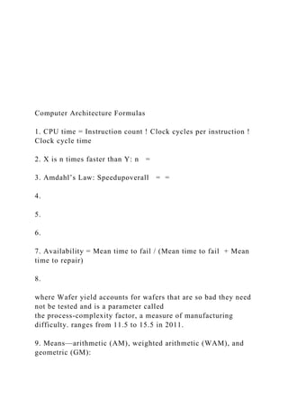
The document outlines key computer architecture formulas and principles, including performance metrics such as CPU time, Amdahl's Law, and memory access times. It discusses the importance of domain-specific architectures in leveraging the slowdown of Moore's Law and the evolving landscape of computer architecture. Additionally, it highlights updates in the sixth edition of 'Computer Architecture: A Quantitative Approach,' emphasizing newly incorporated technology advancements and real-world applications.

1. Computer Architecture Formulas
1. CPU time = Instruction count ! Clock cycles per instruction !
Clock cycle time
2. X is n times faster than Y: n =
3. Amdahl’s Law: Speedupoverall = =
4.
5.
6.
7. Availability = Mean time to fail / (Mean time to fail + Mean
time to repair)
8.
where Wafer yield accounts for wafers that are so bad they need
not be tested and is a parameter called
the process-complexity factor, a measure of manufacturing
difficulty. ranges from 11.5 to 15.5 in 2011.
9. Means—arithmetic (AM), weighted arithmetic (WAM), and
geometric (GM):

2. AM = WAM = GM =
where Timei is the execution time for the ith program of a total
of n in the workload, Weighti is the
weighting of the ith program in the workload.
10. Average memory-access time = Hit time + Miss rate ! Miss
penalty
11. Misses per instruction = Miss rate ! Memory access per
instruction
12. Cache index size: 2index = Cache size /(Block size ! Set
associativity)
13. Power Utilization Effectiveness (PUE) of a Warehouse
Scale Computer =
Rules of Thumb
1. Amdahl/Case Rule: A balanced computer system needs about
1 MB of main memory capacity and 1
megabit per second of I/O bandwidth per MIPS of CPU
performance.
2. 90/10 Locality Rule: A program executes about 90% of its
instructions in 10% of its code.
3. Bandwidth Rule: Bandwidth grows by at least the square of
the improvement in latency.
4. 2:1 Cache Rule: The miss rate of a direct-mapped cache of
size N is about the same as a two-way set-
associative cache of size N/2.
5. Dependability Rule: Design with no single point of failure.

3. 6. Watt-Year Rule: The fully burdened cost of a Watt per year
in a Warehouse Scale Computer in North
America in 2011, including the cost of amortizing the power
and cooling infrastructure, is about $2.
Execution timeY Execution timeX/ PerformanceX
PerformanceY/=
Execution timeold
Execution timenew
-------------------------------------------
1
1 Fractionenhanced–# )
Fractionenhanced
Speedupenhanced
------------------------------------+
---------------------------------------------------------------------------
------------------
Energydynamic 1 2/ Capacitive load Voltage
2
!!
Powerdynamic 1 2/ Capacitive load! Voltage
2 Frequency switched! !
Powerstatic Currentstatic Voltage!
Die yield Wafer yield 1 1 Defects per unit area Die area!+ )(/
N!=

4. 1
n
--- Timei
i 1=
n
Weighti Timei!
i 1=
n n
Timei
i 1=
n
Total Facility Power
IT Equipment Power
--------------------------------------------------
(
N
N
In Praise of Computer Architecture: A Quantitative Approach
Sixth Edition
“Although important concepts of architecture are timeless, this
edition has been
thoroughly updated with the latest technology developments,

5. costs, examples,
and references. Keeping pace with recent developments in open-
sourced architec-
ture, the instruction set architecture used in the book has been
updated to use the
RISC-V ISA.”
—from the foreword by Norman P. Jouppi, Google
“Computer Architecture: A Quantitative Approach is a classic
that, like fine wine,
just keeps getting better. I bought my first copy as I finished up
my undergraduate
degree and it remains one of my most frequently referenced
texts today.”
—James Hamilton, Amazon Web Service
“Hennessy and Patterson wrote the first edition of this book
when graduate stu-
dents built computers with 50,000 transistors. Today,
warehouse-size computers
contain that many servers, each consisting of dozens of
independent processors
and billions of transistors. The evolution of computer
architecture has been rapid
and relentless, butComputer Architecture: A Quantitative
Approach has kept pace,
with each edition accurately explaining and analyzing the
important emerging
ideas that make this field so exciting.”
—James Larus, Microsoft Research
“Another timely and relevant update to a classic, once again
also serving as a win-

6. dow into the relentless and exciting evolution of computer
architecture! The new
discussions in this edition on the slowing of Moore's law and
implications for
future systems are must-reads for both computer architects and
practitioners
working on broader systems.”
—Parthasarathy (Partha) Ranganathan, Google
“I love the ‘Quantitative Approach’ books because they are
written by engineers,
for engineers. John Hennessy and Dave Patterson show the
limits imposed by
mathematics and the possibilities enabled by materials science.
Then they teach
through real-world examples how architects analyze, measure,
and compromise
to build working systems. This sixth edition comes at a critical
time: Moore’s
Law is fading just as deep learning demands unprecedented
compute cycles.
The new chapter on domain-specific architectures documents a
number of prom-
ising approaches and prophesies a rebirth in computer
architecture. Like the
scholars of the European Renaissance, computer architects must
understand our
own history, and then combine the lessons of that history with
new techniques
to remake the world.”
—Cliff Young, Google
She Zinan

7. This page intentionally left blank
Computer Architecture
A Quantitative Approach
Sixth Edition
John L. Hennessy is a Professor of Electrical Engineering and
Computer Science at Stanford
University, where he has been a member of the faculty since
1977 and was, from 2000 to
2016, its 10th President. He currently serves as the Director of
the Knight-Hennessy Fellow-
ship, which provides graduate fellowships to potential future
leaders. Hennessy is a Fellow of
the IEEE and ACM, a member of the National Academy of
Engineering, the National Acad-
emy of Science, and the American Philosophical Society, and a
Fellow of the American Acad-
emy of Arts and Sciences. Among his many awards are the 2001
Eckert-Mauchly Award for
his contributions to RISC technology, the 2001 Seymour Cray
Computer Engineering Award,
and the 2000 John von Neumann Award, which he shared with
David Patterson. He has also
received 10 honorary doctorates.
In 1981, he started the MIPS project at Stanford with a handful
of graduate students. After

8. completing the project in 1984, he took a leave from the
university to cofound MIPS Com-
puter Systems, which developed one of the first commercial
RISC microprocessors. As of
2017, over 5 billion MIPS microprocessors have been shipped in
devices ranging from video
games and palmtop computers to laser printers and network
switches. Hennessy subse-
quently led the DASH (Director Architecture for Shared
Memory) project, which prototyped
the first scalable cache coherent multiprocessor; many of the
key ideas have been adopted
in modern multiprocessors. In addition to his technical
activities and university responsibil-
ities, he has continued to work with numerous start-ups, both as
an early-stage advisor and
an investor.
David A. Patterson became a Distinguished Engineer at Google
in 2016 after 40 years as a
UC Berkeley professor. He joined UC Berkeley immediately
after graduating from UCLA. He
still spends a day a week in Berkeley as an Emeritus Professor
of Computer Science. His
teaching has been honored by the Distinguished Teaching
Award from the University of
California, the Karlstrom Award from ACM, and the Mulligan
Education Medal and Under-
graduate Teaching Award from IEEE. Patterson received the
IEEE Technical Achievement
Award and the ACM Eckert-Mauchly Award for contributions to
RISC, and he shared the IEEE
Johnson Information Storage Award for contributions to RAID.
He also shared the IEEE John
von NeumannMedal and the C & C Prize with John Hennessy.
Like his co-author, Patterson is

9. a Fellow of the American Academy of Arts and Sciences, the
Computer History Museum,
ACM, and IEEE, and he was elected to the National Academy of
Engineering, the National
Academy of Sciences, and the Silicon Valley Engineering Hall
of Fame. He served on the
Information Technology Advisory Committee to the President
of the United States, as chair
of the CS division in the Berkeley EECS department, as chair of
the Computing Research
Association, and as President of ACM. This record led to
Distinguished Service Awards from
ACM, CRA, and SIGARCH. He is currently Vice-Chair of the
Board of Directors of the RISC-V
Foundation.
At Berkeley, Patterson led the design and implementation of
RISC I, likely the first VLSI
reduced instruction set computer, and the foundation of the
commercial SPARC architec-
ture. He was a leader of the Redundant Arrays of Inexpensive
Disks (RAID) project, which led
to dependable storage systems frommany companies. He was
also involved in the Network
of Workstations (NOW) project, which led to cluster technology
used by Internet companies
and later to cloud computing. His current interests are in
designing domain-specific archi-
tectures for machine learning, spreading the word on the open
RISC-V instruction set archi-
tecture, and in helping the UC Berkeley RISELab (Real-time
Intelligent Secure Execution).
Computer Architecture

10. A Quantitative Approach
Sixth Edition
John L. Hennessy
Stanford University
David A. Patterson
University of California, Berkeley
With Contributions by
Krste Asanovi!c
University of California, Berkeley
Jason D. Bakos
University of South Carolina
Robert P. Colwell
R&E Colwell & Assoc. Inc.
Abhishek Bhattacharjee
Rutgers University
Thomas M. Conte
Georgia Tech
Jos!e Duato
Proemisa
Diana Franklin
University of Chicago
David Goldberg
eBay
Norman P. Jouppi
Google
Sheng Li
Intel Labs
Naveen Muralimanohar
HP Labs
Gregory D. Peterson

11. University of Tennessee
Timothy M. Pinkston
University of Southern California
Parthasarathy Ranganathan
Google
David A. Wood
University of Wisconsin–Madison
Cliff Young
Google
Amr Zaky
University of Santa Clara
Morgan Kaufmann is an imprint of Elsevier
50 Hampshire Street, 5th Floor, Cambridge, MA 02139, United
States
© 2019 Elsevier Inc. All rights reserved.
No part of this publication may be reproduced or transmitted in
any form or by any means, electronic or mechanical,
including photocopying, recording, or any information storage
and retrieval system, without permission in writing
from the publisher. Details on how to seek permission, further
information about the Publisher’s permissions
policies and our arrangements with organizations such as the
Copyright Clearance Center and the Copyright
Licensing Agency, can be found at our website:
www.elsevier.com/permissions.
This book and the individual contributions contained in it are
protected under copyright by the Publisher (other than
as may be noted herein).
Notices

12. Knowledge and best practice in this field are constantly
changing. As new research and experience broaden our
understanding, changes in research methods, professional
practices, or medical treatment may become necessary.
Practitioners and researchers must always rely on their own
experience and knowledge in evaluating and using any
information, methods, compounds, or experiments described
herein. In using such information or methods they
should be mindful of their own safety and the safety of others,
including parties for whom they have a professional
responsibility.
To the fullest extent of the law, neither the Publisher nor the
authors, contributors, or editors, assume any liability for
any injury and/or damage to persons or property as a matter of
products liability, negligence or otherwise, or from
any use or operation of any methods, products, instructions, or
ideas contained in the material herein.
Library of Congress Cataloging-in-Publication Data
A catalog record for this book is available from the Library of
Congress
British Library Cataloguing-in-Publication Data
A catalogue record for this book is available from the British
Library
ISBN: 978-0-12-811905-1
For information on all Morgan Kaufmann publications
visit our website at https://www.elsevier.com/books-and-
journals
Publisher: Katey Birtcher
Acquisition Editor: Stephen Merken

13. Developmental Editor: Nate McFadden
Production Project Manager: Stalin Viswanathan
Cover Designer: Christian J. Bilbow
Typeset by SPi Global, India
http://www.elsevier.com/permissions
https://www.elsevier.com/books-and-journals
To Andrea, Linda, and our four sons
This page intentionally left blank
Foreword
by Norman P. Jouppi, Google
Much of the improvement in computer performance over the last
40 years has been
provided by computer architecture advancements that have
leveraged Moore’s
Law and Dennard scaling to build larger and more parallel
systems. Moore’s
Law is the observation that the maximum number of transistors
in an integrated
circuit doubles approximately every two years. Dennard scaling
refers to the reduc-
tion of MOS supply voltage in concert with the scaling of
feature sizes, so that as
transistors get smaller, their power density stays roughly
constant. With the end of

14. Dennard scaling a decade ago, and the recent slowdown of
Moore’s Law due to a
combination of physical limitations and economic factors, the
sixth edition of the
preeminent textbook for our field couldn’t be more timely. Here
are some reasons.
First, because domain-specific architectures can provide
equivalent perfor-
mance and power benefits of three or more historical
generations of Moore’s
Law and Dennard scaling, they now can provide better
implementations than
may ever be possible with future scaling of general-purpose
architectures. And
with the diverse application space of computers today, there are
many potential
areas for architectural innovation with domain-specific
architectures. Second,
high-quality implementations of open-source architectures now
have a much lon-
ger lifetime due to the slowdown in Moore’s Law. This gives
them more oppor-
tunities for continued optimization and refinement, and hence
makes them more
attractive. Third, with the slowing of Moore’s Law, different
technology compo-
nents have been scaling heterogeneously. Furthermore, new
technologies such as
2.5D stacking, new nonvolatile memories, and optical
interconnects have been
developed to provide more than Moore’s Law can supply alone.
To use these
new technologies and nonhomogeneous scaling effectively,
fundamental design
decisions need to be reexamined from first principles. Hence it

15. is important for
students, professors, and practitioners in the industry to be
skilled in a wide range
of both old and new architectural techniques. All told, I believe
this is the most
exciting time in computer architecture since the industrial
exploitation of
instruction-level parallelism in microprocessors 25 years ago.
The largest change in this edition is the addition of a new
chapter on domain-
specific architectures. It’s long been known that customized
domain-specific archi-
tectures can have higher performance, lower power, and require
less silicon area
than general-purpose processor implementations. However when
general-purpose
ix
processors were increasing in single-threaded performance by
40% per year (see
Fig. 1.11), the extra time to market required to develop a
custom architecture vs.
using a leading-edge standard microprocessor could cause the
custom architecture
to lose much of its advantage. In contrast, today single-core
performance is
improving very slowly, meaning that the benefits of custom
architectures will
not be made obsolete by general-purpose processors for a very
long time, if ever.
Chapter 7 covers several domain-specific architectures. Deep
neural networks

16. have very high computation requirements but lower data
precision requirements –
this combination can benefit significantly from custom
architectures. Two example
architectures and implementations for deep neural networks are
presented: one
optimized for inference and a second optimized for training.
Image processing
is another example domain; it also has high computation
demands and benefits
from lower-precision data types. Furthermore, since it is often
found in mobile
devices, the power savings from custom architectures are also
very valuable.
Finally, by nature of their reprogrammability, FPGA-based
accelerators can be
used to implement a variety of different domain-specific
architectures on a single
device. They also can benefit more irregular applications that
are frequently
updated, like accelerating internet search.
Although important concepts of architecture are timeless, this
edition has been
thoroughly updated with the latest technology developments,
costs, examples, and
references. Keeping pace with recent developments in open-
sourced architecture,
the instruction set architecture used in the book has been
updated to use the
RISC-V ISA.
On a personal note, after enjoying the privilege of working with
John as a grad-
uate student, I am now enjoying the privilege of working with
Dave at Google.

17. What an amazing duo!
x ■ Foreword
Contents
Foreword ix
Preface xvii
Acknowledgments xxv
Chapter 1 Fundamentals of Quantitative Design and Analysis
1.1 Introduction 2
1.2 Classes of Computers 6
1.3 Defining Computer Architecture 11
1.4 Trends in Technology 18
1.5 Trends in Power and Energy in Integrated Circuits 23
1.6 Trends in Cost 29
1.7 Dependability 36
1.8 Measuring, Reporting, and Summarizing Performance 39
1.9 Quantitative Principles of Computer Design 48
1.10 Putting It All Together: Performance, Price, and Power 55
1.11 Fallacies and Pitfalls 58
1.12 Concluding Remarks 64
1.13 Historical Perspectives and References 67
Case Studies and Exercises by Diana Franklin 67
Chapter 2 Memory Hierarchy Design
2.1 Introduction 78
2.2 Memory Technology and Optimizations 84

18. 2.3 Ten Advanced Optimizations of Cache Performance 94
2.4 Virtual Memory and Virtual Machines 118
2.5 Cross-Cutting Issues: The Design of Memory Hierarchies
126
2.6 Putting It All Together: Memory Hierarchies in the ARM
Cortex-A53
and Intel Core i7 6700 129
2.7 Fallacies and Pitfalls 142
2.8 Concluding Remarks: Looking Ahead 146
2.9 Historical Perspectives and References 148
xi
Case Studies and Exercises by Norman P. Jouppi, Rajeev
Balasubramonian, Naveen Muralimanohar, and Sheng Li 148
Chapter 3 Instruction-Level Parallelism and Its Exploitation
3.1 Instruction-Level Parallelism: Concepts and Challenges 168
3.2 Basic Compiler Techniques for Exposing ILP 176
3.3 Reducing Branch Costs With Advanced Branch Prediction
182
3.4 Overcoming Data Hazards With Dynamic Scheduling 191
3.5 Dynamic Scheduling: Examples and the Algorithm 201
3.6 Hardware-Based Speculation 208
3.7 Exploiting ILP Using Multiple Issue and Static Scheduling
218
3.8 Exploiting ILP Using Dynamic Scheduling, Multiple Issue,
and
Speculation 222
3.9 Advanced Techniques for Instruction Delivery and
Speculation 228

19. 3.10 Cross-Cutting Issues 240
3.11 Multithreading: Exploiting Thread-Level Parallelism to
Improve
Uniprocessor Throughput 242
3.12 Putting It All Together: The Intel Core i7 6700 and ARM
Cortex-A53 247
3.13 Fallacies and Pitfalls 258
3.14 Concluding Remarks: What’s Ahead? 264
3.15 Historical Perspective and References 266
Case Studies and Exercises by Jason D. Bakos and Robert P.
Colwell 266
Chapter 4 Data-Level Parallelism in Vector, SIMD, and GPU
Architectures
4.1 Introduction 282
4.2 Vector Architecture 283
4.3 SIMD Instruction Set Extensions for Multimedia 304
4.4 Graphics Processing Units 310
4.5 Detecting and Enhancing Loop-Level Parallelism 336
4.6 Cross-Cutting Issues 345
4.7 Putting It All Together: Embedded Versus Server GPUs and
Tesla Versus Core i7 346
4.8 Fallacies and Pitfalls 353
4.9 Concluding Remarks 357
4.10 Historical Perspective and References 357
Case Study and Exercises by Jason D. Bakos 357
Chapter 5 Thread-Level Parallelism
5.1 Introduction 368
5.2 Centralized Shared-Memory Architectures 377

20. 5.3 Performance of Symmetric Shared-Memory Multiprocessors
393
xii ■ Contents
5.4 Distributed Shared-Memory and Directory-Based Coherence
404
5.5 Synchronization: The Basics 412
5.6 Models of Memory Consistency: An Introduction 417
5.7 Cross-Cutting Issues 422
5.8 Putting It All Together: Multicore Processors and Their
Performance 426
5.9 Fallacies and Pitfalls 438
5.10 The Future of Multicore Scaling 442
5.11 Concluding Remarks 444
5.12 Historical Perspectives and References 445
Case Studies and Exercises by Amr Zaky and David A. Wood
446
Chapter 6 Warehouse-Scale Computers to Exploit Request-
Level
and Data-Level Parallelism
6.1 Introduction 466
6.2 Programming Models and Workloads for Warehouse-Scale
Computers 471
6.3 Computer Architecture of Warehouse-Scale Computers 477
6.4 The Efficiency and Cost of Warehouse-Scale Computers 482
6.5 Cloud Computing: The Return of Utility Computing 490
6.6 Cross-Cutting Issues 501
6.7 Putting It All Together: A Google Warehouse-Scale
Computer 503

21. 6.8 Fallacies and Pitfalls 514
6.9 Concluding Remarks 518
6.10 Historical Perspectives and References 519
Case Studies and Exercises by Parthasarathy Ranganathan 519
Chapter 7 Domain-Specific Architectures
7.1 Introduction 540
7.2 Guidelines for DSAs 543
7.3 Example Domain: Deep Neural Networks 544
7.4 Google’s Tensor Processing Unit, an Inference Data
Center Accelerator 557
7.5 Microsoft Catapult, a Flexible Data Center Accelerator 567
7.6 Intel Crest, a Data Center Accelerator for Training 579
7.7 Pixel Visual Core, a Personal Mobile Device Image
Processing Unit 579
7.8 Cross-Cutting Issues 592
7.9 Putting It All Together: CPUs Versus GPUs Versus DNN
Accelerators 595
7.10 Fallacies and Pitfalls 602
7.11 Concluding Remarks 604
7.12 Historical Perspectives and References 606
Case Studies and Exercises by Cliff Young 606
Contents ■ xiii
Appendix A Instruction Set Principles
A.1 Introduction A-2
A.2 Classifying Instruction Set Architectures A-3
A.3 Memory Addressing A-7

22. A.4 Type and Size of Operands A-13
A.5 Operations in the Instruction Set A-15
A.6 Instructions for Control Flow A-16
A.7 Encoding an Instruction Set A-21
A.8 Cross-Cutting Issues: The Role of Compilers A-24
A.9 Putting It All Together: The RISC-V Architecture A-33
A.10 Fallacies and Pitfalls A-42
A.11 Concluding Remarks A-46
A.12 Historical Perspective and References A-47
Exercises by Gregory D. Peterson A-47
Appendix B Review of Memory Hierarchy
B.1 Introduction B-2
B.2 Cache Performance B-15
B.3 Six Basic Cache Optimizations B-22
B.4 Virtual Memory B-40
B.5 Protection and Examples of Virtual Memory B-49
B.6 Fallacies and Pitfalls B-57
B.7 Concluding Remarks B-59
B.8 Historical Perspective and References B-59
Exercises by Amr Zaky B-60
Appendix C Pipelining: Basic and Intermediate Concepts
C.1 Introduction C-2
C.2 The Major Hurdle of Pipelining—Pipeline Hazards C-10
C.3 How Is Pipelining Implemented? C-26
C.4 What Makes Pipelining Hard to Implement? C-37
C.5 Extending the RISC V Integer Pipeline to Handle
Multicycle
Operations C-45
C.6 Putting It All Together: The MIPS R4000 Pipeline C-55

23. C.7 Cross-Cutting Issues C-65
C.8 Fallacies and Pitfalls C-70
C.9 Concluding Remarks C-71
C.10 Historical Perspective and References C-71
Updated Exercises by Diana Franklin C-71
xiv ■ Contents
Online Appendices
Appendix D Storage Systems
Appendix E Embedded Systems
by Thomas M. Conte
Appendix F Interconnection Networks
by Timothy M. Pinkston and Jos!e Duato
Appendix G Vector Processors in More Depth
by Krste Asanovic
Appendix H Hardware and Software for VLIW and EPIC
Appendix I Large-Scale Multiprocessors and Scientific
Applications
Appendix J Computer Arithmetic
by David Goldberg
Appendix K Survey of Instruction Set Architectures
Appendix L Advanced Concepts on Address Translation
by Abhishek Bhattacharjee

24. Appendix M Historical Perspectives and References
References R-1
Index I-1
Contents ■ xv
This page intentionally left blank
Preface
Why We Wrote This Book
Through six editions of this book, our goal has been to describe
the basic principles
underlying what will be tomorrow’s technological
developments. Our excitement
about the opportunities in computer architecture has not abated,
and we echo what
we said about the field in the first edition: “It is not a dreary
science of paper
machines that will never work. No! It’s a discipline of keen
intellectual interest,
requiring the balance of marketplace forces to cost-
performance-power, leading
to glorious failures and some notable successes.”
Our primary objective in writing our first book was to change
the way people
learn and think about computer architecture. We feel this goal is

25. still valid and
important. The field is changing daily and must be studied with
real examples
and measurements on real computers, rather than simply as a
collection of defini-
tions and designs that will never need to be realized. We offer
an enthusiastic wel-
come to anyone who came along with us in the past, as well as
to those who are
joining us now. Either way, we can promise the same
quantitative approach to, and
analysis of, real systems.
As with earlier versions, we have strived to produce a new
edition that will
continue to be as relevant for professional engineers and
architects as it is for those
involved in advanced computer architecture and design courses.
Like the first edi-
tion, this edition has a sharp focus on new platforms—personal
mobile devices and
warehouse-scale computers—and new architectures—
specifically, domain-
specific architectures. As much as its predecessors, this edition
aims to demystify
computer architecture through an emphasis on cost-
performance-energy trade-offs
and good engineering design. We believe that the field has
continued to mature and
move toward the rigorous quantitative foundation of long-
established scientific
and engineering disciplines.
xvii

26. This Edition
The ending of Moore’s Law and Dennard scaling is having as
profound effect on
computer architecture as did the switch to multicore. We retain
the focus on the
extremes in size of computing, with personal mobile devices
(PMDs) such as cell
phones and tablets as the clients and warehouse-scale computers
offering cloud
computing as the server. We also maintain the other theme of
parallelism in all
its forms: data-level parallelism (DLP) in Chapters 1 and 4,
instruction-level par-
allelism (ILP) in Chapter 3, thread-level parallelism in Chapter
5, and request-
level parallelism (RLP) in Chapter 6.
The most pervasive change in this edition is switching
fromMIPS to the RISC-
V instruction set. We suspect this modern, modular, open
instruction set may
become a significant force in the information technology
industry. It may become
as important in computer architecture as Linux is for operating
systems.
The newcomer in this edition is Chapter 7, which introduces
domain-specific
architectures with several concrete examples from industry.
As before, the first three appendices in the book give basics on
the RISC-V
instruction set, memory hierarchy, and pipelining for readers
who have not read

27. a book like Computer Organization and Design. To keep costs
down but still sup-
ply supplemental material that is of interest to some readers,
available online at
https://www.elsevier.com/books-and-journals/book-
companion/9780128119051
are nine more appendices. There are more pages in these
appendices than there are
in this book!
This edition continues the tradition of using real-world
examples to demonstrate
the ideas, and the “Putting ItAll Together” sections are brand
new.The “Putting ItAll
Together” sectionsof this edition include
thepipelineorganizationsandmemoryhier-
archies of the ARM Cortex A8 processor, the Intel core i7
processor, the NVIDIA
GTX-280 and GTX-480 GPUs, and one of the Google
warehouse-scale computers.
Topic Selection and Organization
As before, we have taken a conservative approach to topic
selection, for there are
many more interesting ideas in the field than can reasonably be
covered in a treat-
ment of basic principles. We have steered away from a
comprehensive survey of
every architecture a reader might encounter. Instead, our
presentation focuses on
core concepts likely to be found in any new machine. The key
criterion remains
that of selecting ideas that have been examined and utilized
successfully enough
to permit their discussion in quantitative terms.

28. Our intent has always been to focus on material that is not
available in equiv-
alent form from other sources, so we continue to emphasize
advanced content
wherever possible. Indeed, there are several systems here whose
descriptions can-
not be found in the literature. (Readers interested strictly in a
more basic introduc-
tion to computer architecture should readComputer Organization
and Design: The
Hardware/Software Interface.)
xviii ■ Preface
https://www.elsevier.com/books-and-journals/book-
companion/9780128119051
An Overview of the Content
Chapter 1 includes formulas for energy, static power, dynamic
power, integrated cir-
cuit costs, reliability, and availability. (These formulas are also
found on the front
inside cover.) Our hope is that these topics can be used through
the rest of the book.
In addition to the classic quantitative principles of computer
design and performance
measurement, it shows the slowing of performance improvement
of general-purpose
microprocessors, which is one inspiration for domain-specific
architectures.
Our view is that the instruction set architecture is playing less
of a role today

29. than in 1990, so we moved this material to Appendix A. It now
uses the RISC-V
architecture. (For quick review, a summary of the RISC-V ISA
can be found on the
back inside cover.) For fans of ISAs, Appendix K was revised
for this edition and
covers 8 RISC architectures (5 for desktop and server use and 3
for embedded use),
the 80!86, the DEC VAX, and the IBM 360/370.
We then move onto memory hierarchy in Chapter 2, since it is
easy to apply the
cost-performance-energy principles to this material, and
memory is a critical
resource for the rest of the chapters. As in the past edition,
Appendix B contains
an introductory review of cache principles, which is available in
case you need it.
Chapter 2 discusses 10 advanced optimizations of caches. The
chapter includes
virtual machines, which offer advantages in protection, software
management,
and hardware management, and play an important role in cloud
computing. In
addition to covering SRAM and DRAM technologies, the
chapter includes new
material both on Flash memory and on the use of stacked die
packaging for extend-
ing the memory hierarchy. The PIAT examples are the ARM
Cortex A8, which is
used in PMDs, and the Intel Core i7, which is used in servers.
Chapter 3 covers the exploitation of instruction-level
parallelism in high-
performance processors, including superscalar execution,
branch prediction

30. (including the new tagged hybrid predictors), speculation,
dynamic scheduling,
and simultaneous multithreading. As mentioned earlier,
Appendix C is a review
of pipelining in case you need it. Chapter 3 also surveys the
limits of ILP. Like
Chapter 2, the PIAT examples are again the ARM Cortex A8
and the Intel Core
i7. While the third edition contained a great deal on Itanium and
VLIW, this mate-
rial is now in Appendix H, indicating our view that this
architecture did not live up
to the earlier claims.
The increasing importance of multimedia applications such as
games and video
processing has also increased the importance of architectures
that can exploit data
level parallelism. In particular, there is a rising interest in
computing using graph-
ical processing units (GPUs), yet few architects understand
howGPUs really work.
We decided to write a new chapter in large part to unveil this
new style of computer
architecture. Chapter 4 starts with an introduction to vector
architectures, which
acts as a foundation on which to build explanations of
multimedia SIMD instruc-
tion set extensions and GPUs. (Appendix G goes into even more
depth on vector
architectures.) This chapter introduces the Roofline
performance model and then
uses it to compare the Intel Core i7 and the NVIDIAGTX 280
andGTX 480GPUs.
The chapter also describes the Tegra 2 GPU for PMDs.

31. Preface ■ xix
Chapter 5 describes multicore processors. It explores symmetric
and
distributed-memory architectures, examining both
organizational principles and
performance. The primary additions to this chapter include more
comparison of
multicore organizations, including the organization of
multicore-multilevel
caches, multicore coherence schemes, and on-chip multicore
interconnect. Topics
in synchronization and memory consistency models are next.
The example is the
Intel Core i7. Readers interested in more depth on
interconnection networks should
read Appendix F, and those interested in larger scale
multiprocessors and scientific
applications should read Appendix I.
Chapter 6 describes warehouse-scale computers (WSCs). It was
extensively
revised based on help from engineers at Google and Amazon
Web Services. This
chapter integrates details on design, cost, and performance
ofWSCs that few archi-
tects are aware of. It starts with the popular MapReduce
programming model
before describing the architecture and physical implementation
of WSCs, includ-
ing cost. The costs allow us to explain the emergence of cloud
computing, whereby
it can be cheaper to compute usingWSCs in the cloud than in
your local datacenter.

32. The PIAT example is a description of a Google WSC that
includes information
published for the first time in this book.
The new Chapter 7 motivates the need for Domain-Specific
Architectures
(DSAs). It draws guiding principles for DSAs based on the four
examples of DSAs.
EachDSAcorresponds to chips that have been deployed in
commercial settings.We
also explain why we expect a renaissance in computer
architecture via DSAs given
that single-thread performance of general-purpose
microprocessors has stalled.
This brings us to Appendices A through M. Appendix A covers
principles of
ISAs, including RISC-V, and Appendix K describes 64-bit
versions of RISC V,
ARM,MIPS, Power, and SPARC and their multimedia
extensions. It also includes
some classic architectures (80x86, VAX, and IBM 360/370) and
popular embed-
ded instruction sets (Thumb-2, microMIPS, and RISCVC).
Appendix H is related,
in that it covers architectures and compilers for VLIW ISAs.
As mentioned earlier, Appendix B and Appendix C are tutorials
on basic cach-
ing and pipelining concepts. Readers relatively new to caching
should read Appen-
dix B before Chapter 2, and those new to pipelining should read
Appendix C before
Chapter 3.
Appendix D, “Storage Systems,” has an expanded discussion of

33. reliability and
availability, a tutorial on RAID with a description of RAID 6
schemes, and rarely
found failure statistics of real systems. It continues to provide
an introduction to
queuing theory and I/O performance benchmarks. We evaluate
the cost, perfor-
mance, and reliability of a real cluster: the Internet Archive.
The “Putting It All
Together” example is the NetApp FAS6000 filer.
Appendix E, by Thomas M. Conte, consolidates the embedded
material in
one place.
Appendix F, on interconnection networks, is revised by Timothy
M. Pinkston
and Jos!e Duato. Appendix G, written originally by Krste
Asanovi!c, includes a
description of vector processors. We think these two appendices
are some of
the best material we know of on each topic.
xx ■ Preface
Appendix H describes VLIW and EPIC, the architecture of
Itanium.
Appendix I describes parallel processing applications and
coherence protocols
for larger-scale, shared-memory multiprocessing. Appendix J,
by David Goldberg,
describes computer arithmetic.

34. Appendix L, by Abhishek Bhattacharjee, is new and discusses
advanced tech-
niques for memory management, focusing on support for virtual
machines and
design of address translation for very large address spaces. With
the growth in
clouds processors, these architectural enhancements are
becoming more important.
Appendix M collects the “Historical Perspective and
References” from each
chapter into a single appendix. It attempts to give proper credit
for the ideas in each
chapter and a sense of the history surrounding the inventions.
We like to think of
this as presenting the human drama of computer design. It also
supplies references
that the student of architecture may want to pursue. If you have
time, we recom-
mend reading some of the classic papers in the field that are
mentioned in these
sections. It is both enjoyable and educational to hear the ideas
directly from the
creators. “Historical Perspective” was one of the most popular
sections of prior
editions.
Navigating the Text
There is no single best order in which to approach these
chapters and appendices,
except that all readers should start with Chapter 1. If you don’t
want to read every-
thing, here are some suggested sequences:
■ Memory Hierarchy: Appendix B, Chapter 2, and Appendices

35. D and M.
■ Instruction-Level Parallelism: Appendix C, Chapter 3, and
Appendix H
■ Data-Level Parallelism: Chapters 4, 6, and 7, Appendix G
■ Thread-Level Parallelism: Chapter 5, Appendices F and I
■ Request-Level Parallelism: Chapter 6
■ ISA: Appendices A and K
Appendix E can be read at any time, but it might work best if
read after the ISA and
cache sequences. Appendix J can be read whenever arithmetic
moves you. You
should read the corresponding portion of Appendix M after you
complete each
chapter.
Chapter Structure
The material we have selected has been stretched upon a
consistent framework that
is followed in each chapter. We start by explaining the ideas of
a chapter. These
ideas are followed by a “Crosscutting Issues” section, a feature
that shows how the
ideas covered in one chapter interact with those given in other
chapters. This is
Preface ■ xxi

36. followed by a “Putting It All Together” section that ties these
ideas together by
showing how they are used in a real machine.
Next in the sequence is “Fallacies and Pitfalls,” which lets
readers learn from
the mistakes of others. We show examples of common
misunderstandings and
architectural traps that are difficult to avoid even when you
know they are lying
in wait for you. The “Fallacies and Pitfalls” sections is one of
the most popular
sections of the book. Each chapter ends with a “Concluding
Remarks” section.
Case Studies With Exercises
Each chapter ends with case studies and accompanying
exercises. Authored by
experts in industry and academia, the case studies explore key
chapter concepts
and verify understanding through increasingly challenging
exercises. Instructors
should find the case studies sufficiently detailed and robust to
allow them to create
their own additional exercises.
Brackets for each exercise (<chapter.section>) indicate the text
sections of
primary relevance to completing the exercise. We hope this
helps readers to avoid
exercises for which they haven’t read the corresponding section,
in addition to pro-
viding the source for review. Exercises are rated, to give the
reader a sense of the
amount of time required to complete an exercise:

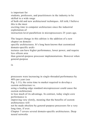
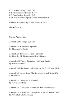
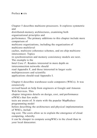
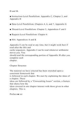
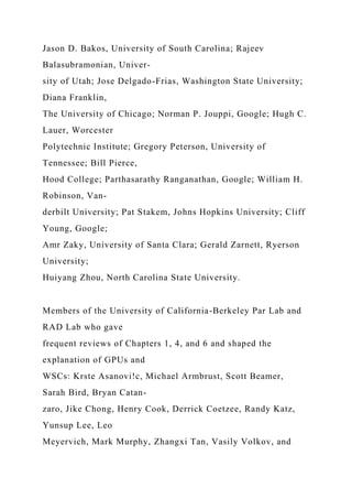
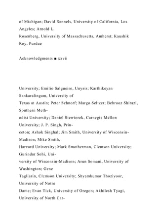
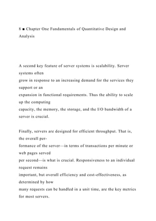
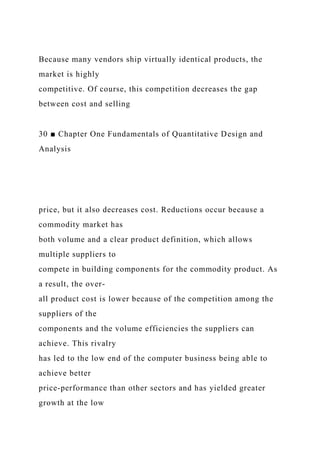
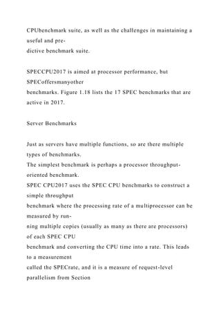
37. [10] Less than 5 min (to read and understand)
[15] 5–15 min for a full answer
[20] 15–20 min for a full answer
[25] 1 h for a full written answer
[30] Short programming project: less than 1 full day of
programming
[40] Significant programming project: 2 weeks of elapsed time
[Discussion] Topic for discussion with others
Solution
s to the case studies and exercises are available for instructors
who
register at textbooks.elsevier.com.
Supplemental Materials
A variety of resources are available online at
https://www.elsevier.com/books/
computer-architecture/hennessy/978-0-12-811905-1, including
the following:

38. ■ Reference appendices, some guest authored by subject
experts, covering a
range of advanced topics
■ Historical perspectives material that explores the development
of the key ideas
presented in each of the chapters in the text
xxii ■ Preface
https://www.elsevier.com/books/computer-
architecture/hennessy/978-0-12-811905-1
https://www.elsevier.com/books/computer-
architecture/hennessy/978-0-12-811905-1
■ Instructor slides in PowerPoint
■ Figures from the book in PDF, EPS, and PPT formats
■ Links to related material on the Web
■ List of errata

39. New materials and links to other resources available on the Web
will be added
on a regular basis.
Helping Improve This Book
Finally, it is possible to make money while reading this book.
(Talk about cost per-
formance!) If you read the Acknowledgments that follow, you
will see that we
went to great lengths to correct mistakes. Since a book goes
through many print-
ings, we have the opportunity to make even more corrections. If
you uncover any
remaining resilient bugs, please contact the publisher by
electronic mail
([email protected]).
We welcome general comments to the text and invite you to
send them to a
separate email address at [email protected]
Concluding Remarks
Once again, this book is a true co-authorship, with each of us
writing half the chap-

40. ters and an equal share of the appendices.We can’t imagine how
long it would have
taken without someone else doing half the work, offering
inspiration when the task
seemed hopeless, providing the key insight to explain a difficult
concept, supply-
ing over-the-weekend reviews of chapters, and commiserating
when the weight of
our other obligations made it hard to pick up the pen.
Thus, once again, we share equally the blame for what you are
about to read.
John Hennessy ■ David Patterson
Preface ■ xxiii
mailto:[email protected]
mailto:[email protected]
mailto:[email protected]
mailto:[email protected]
This page intentionally left blank

41. Acknowledgments
Although this is only the sixth edition of this book, we have
actually created ten
different versions of the text: three versions of the first edition
(alpha, beta, and
final) and two versions of the second, third, and fourth editions
(beta and final).
Along the way, we have received help from hundreds of
reviewers and users. Each
of these people has helped make this book better. Thus, we have
chosen to list all of
the people who have made contributions to some version of this
book.
Contributors to the Sixth Edition
Like prior editions, this is a community effort that involves
scores of volunteers.
Without their help, this edition would not be nearly as polished.
Reviewers

42. Jason D. Bakos, University of South Carolina; Rajeev
Balasubramonian, Univer-
sity of Utah; Jose Delgado-Frias, Washington State University;
Diana Franklin,
The University of Chicago; Norman P. Jouppi, Google; Hugh C.
Lauer, Worcester
Polytechnic Institute; Gregory Peterson, University of
Tennessee; Bill Pierce,
Hood College; Parthasarathy Ranganathan, Google; William H.
Robinson, Van-
derbilt University; Pat Stakem, Johns Hopkins University; Cliff
Young, Google;
Amr Zaky, University of Santa Clara; Gerald Zarnett, Ryerson
University;
Huiyang Zhou, North Carolina State University.
Members of the University of California-Berkeley Par Lab and
RAD Lab who gave
frequent reviews of Chapters 1, 4, and 6 and shaped the
explanation of GPUs and
WSCs: Krste Asanovi!c, Michael Armbrust, Scott Beamer,
Sarah Bird, Bryan Catan-
zaro, Jike Chong, Henry Cook, Derrick Coetzee, Randy Katz,
Yunsup Lee, Leo
Meyervich, Mark Murphy, Zhangxi Tan, Vasily Volkov, and

43. Andrew Waterman.
Appendices
Krste Asanovi!c, University of California, Berkeley (Appendix
G); Abhishek
Bhattacharjee, Rutgers University (Appendix L); Thomas M.
Conte, North Caro-
lina State University (Appendix E); Jos!e Duato, Universitat
Politècnica de
xxv
València and Simula (Appendix F); David Goldberg, Xerox
PARC (Appendix J);
Timothy M. Pinkston, University of Southern California
(Appendix F).
Jos!e Flich of the Universidad Polit!ecnica de Valencia
provided significant contri-
butions to the updating of Appendix F.
Case Studies With Exercises

44. Jason D. Bakos, University of South Carolina (Chapters 3 and
4); Rajeev Balasu-
bramonian, University of Utah (Chapter 2); Diana Franklin, The
University of
Chicago (Chapter 1 and Appendix C); Norman P. Jouppi,
Google, (Chapter 2);
Naveen Muralimanohar, HP Labs (Chapter 2); Gregory
Peterson, University of
Tennessee (Appendix A); Parthasarathy Ranganathan, Google
(Chapter 6); Cliff
Young, Google (Chapter 7); Amr Zaky, University of Santa
Clara (Chapter 5
and Appendix B).
Jichuan Chang, Junwhan Ahn, Rama Govindaraju, and Milad
Hashemi assisted in
the development and testing of the case studies and exercises
for Chapter 6.
Additional Material
John Nickolls, Steve Keckler, and Michael Toksvig of NVIDIA
(Chapter 4 NVI-
DIA GPUs); Victor Lee, Intel (Chapter 4 comparison of Core i7

45. and GPU); John
Shalf, LBNL (Chapter 4 recent vector architectures);
SamWilliams, LBNL (Roof-
line model for computers in Chapter 4); Steve Blackburn of
Australian National
University and Kathryn McKinley of University of Texas at
Austin (Intel perfor-
mance and power measurements in Chapter 5); Luiz Barroso,
Urs H€olzle, Jimmy
Clidaris, Bob Felderman, and Chris Johnson of Google (the
Google WSC in
Chapter 6); James Hamilton of AmazonWeb Services (power
distribution and cost
model in Chapter 6).
Jason D. Bakos of the University of South Carolina updated the
lecture slides
for this edition.
This book could not have been published without a publisher, of
course. We
wish to thank all the Morgan Kaufmann/Elsevier staff for their
efforts and support.
For this fifth edition, we particularly want to thank our editors
Nate McFadden and

46. SteveMerken, who coordinated surveys, development of the case
studies and exer-
cises, manuscript reviews, and the updating of the appendices.
We must also thank our university staff, Margaret Rowland and
Roxana
Infante, for countless express mailings, as well as for holding
down the fort at Stan-
ford and Berkeley while we worked on the book.
Our final thanks go to our wives for their suffering through
increasingly early
mornings of reading, thinking, and writing.
xxvi ■ Acknowledgments
Contributors to Previous Editions
Reviewers
George Adams, Purdue University; Sarita Adve, University of
Illinois at Urbana-
Champaign; Jim Archibald, Brigham Young University; Krste

47. Asanovi!c, Massa-
chusetts Institute of Technology; Jean-Loup Baer, University of
Washington; Paul
Barr, Northeastern University; Rajendra V. Boppana, University
of Texas, San
Antonio; Mark Brehob, University of Michigan; Doug Burger,
University of
Texas, Austin; John Burger, SGI; Michael Butler; Thomas
Casavant; Rohit Chan-
dra; Peter Chen, University of Michigan; the classes at SUNY
Stony Brook, Car-
negie Mellon, Stanford, Clemson, and Wisconsin; Tim Coe,
Vitesse
Semiconductor; Robert P. Colwell; David Cummings; Bill
Dally; David Douglas;
Jos!e Duato, Universitat Politècnica de València and Simula;
Anthony Duben,
Southeast Missouri State University; Susan Eggers, University
of Washington;
Joel Emer; Barry Fagin, Dartmouth; Joel Ferguson, University
of California, Santa
Cruz; Carl Feynman; David Filo; Josh Fisher, Hewlett-Packard
Laboratories; Rob
Fowler, DIKU; Mark Franklin, Washington University (St.
Louis); Kourosh Ghar-

48. achorloo; Nikolas Gloy, Harvard University; David Goldberg,
Xerox Palo Alto
Research Center; Antonio González, Intel and Universitat
Politècnica de Catalu-
nya; James Goodman, University of Wisconsin-Madison;
Sudhanva Gurumurthi,
University of Virginia; David Harris, Harvey Mudd College;
John Heinlein; Mark
Heinrich, Stanford; Daniel Helman, University of California,
Santa Cruz; Mark D.
Hill, University of Wisconsin-Madison; Martin Hopkins, IBM;
Jerry Huck,
Hewlett-Packard Laboratories; Wen-mei Hwu, University of
Illinois at Urbana-
Champaign; Mary Jane Irwin, Pennsylvania State University;
Truman Joe; Norm
Jouppi; David Kaeli, Northeastern University; Roger
Kieckhafer, University of
Nebraska; Lev G. Kirischian, Ryerson University; Earl Killian;
Allan Knies, Pur-
due University; Don Knuth; Jeff Kuskin, Stanford; James R.
Larus, Microsoft
Research; Corinna Lee, University of Toronto; Hank Levy; Kai
Li, Princeton Uni-
versity; Lori Liebrock, University of Alaska, Fairbanks; Mikko

49. Lipasti, University
of Wisconsin-Madison; Gyula A. Mago, University of North
Carolina, Chapel
Hill; BryanMartin; NormanMatloff;
DavidMeyer;WilliamMichalson,Worcester
Polytechnic Institute; James Mooney; Trevor Mudge, University
of Michigan;
Ramadass Nagarajan, University of Texas at Austin; David
Nagle, Carnegie Mel-
lon University; Todd Narter; Victor Nelson; Vojin Oklobdzija,
University of Cal-
ifornia, Berkeley; Kunle Olukotun, Stanford University; Bob
Owens,
Pennsylvania State University; Greg Papadapoulous, Sun
Microsystems; Joseph
Pfeiffer; Keshav Pingali, Cornell University; Timothy M.
Pinkston, University
of Southern California; Bruno Preiss, University of Waterloo;
Steven Przybylski;
Jim Quinlan; Andras Radics; Kishore Ramachandran, Georgia
Institute of Tech-
nology; Joseph Rameh, University of Texas, Austin; Anthony
Reeves, Cornell
University; Richard Reid, Michigan State University; Steve
Reinhardt, University

50. of Michigan; David Rennels, University of California, Los
Angeles; Arnold L.
Rosenberg, University of Massachusetts, Amherst; Kaushik
Roy, Purdue
Acknowledgments ■ xxvii
University; Emilio Salgueiro, Unysis; Karthikeyan
Sankaralingam, University of
Texas at Austin; Peter Schnorf; Margo Seltzer; Behrooz Shirazi,
Southern Meth-
odist University; Daniel Siewiorek, Carnegie Mellon
University; J. P. Singh, Prin-
ceton; Ashok Singhal; Jim Smith, University of Wisconsin-
Madison; Mike Smith,
Harvard University; Mark Smotherman, Clemson University;
Gurindar Sohi, Uni-
versity of Wisconsin-Madison; Arun Somani, University of
Washington; Gene
Tagliarin, Clemson University; Shyamkumar Thoziyoor,
University of Notre
Dame; Evan Tick, University of Oregon; Akhilesh Tyagi,
University of North Car-

51. olina, Chapel Hill; Dan Upton, University of Virginia; Mateo
Valero, Universidad
Polit!ecnica de Cataluña, Barcelona; Anujan Varma, University
of California, Santa
Cruz; Thorsten von Eicken, Cornell University; Hank Walker,
Texas A&M; Roy
Want, Xerox Palo Alto Research Center; David Weaver, Sun
Microsystems;
ShlomoWeiss, Tel Aviv University; DavidWells; MikeWestall,
Clemson Univer-
sity; Maurice Wilkes; Eric Williams; Thomas Willis, Purdue
University; Malcolm
Wing; Larry Wittie, SUNY Stony Brook; Ellen Witte Zegura,
Georgia Institute of
Technology; Sotirios G. Ziavras, New Jersey Institute of
Technology.
Appendices
The vector appendix was revised by Krste Asanovi!c of the
Massachusetts Institute
of Technology. The floating-point appendix was written
originally by David Gold-
berg of Xerox PARC.

52. Exercises
George Adams, Purdue University; Todd M. Bezenek,
University of Wisconsin-
Madison (in remembrance of his grandmother Ethel Eshom);
Susan Eggers;
Anoop Gupta; David Hayes; Mark Hill; Allan Knies; Ethan L.
Miller, University
of California, Santa Cruz; Parthasarathy Ranganathan, Compaq
Western Research
Laboratory; Brandon Schwartz, University of Wisconsin-
Madison; Michael Scott;
Dan Siewiorek; Mike Smith; Mark Smotherman; Evan Tick;
Thomas Willis.
Case Studies With Exercises
Andrea C. Arpaci-Dusseau, University of Wisconsin-Madison;
Remzi H. Arpaci-
Dusseau, University of Wisconsin-Madison; Robert P. Colwell,
R&E Colwell &
Assoc., Inc.; Diana Franklin, California Polytechnic State
University, San Luis
Obispo; Wen-mei W. Hwu, University of Illinois at Urbana-
Champaign; Norman

53. P. Jouppi, HP Labs; John W. Sias, University of Illinois at
Urbana-Champaign;
David A. Wood, University of Wisconsin-Madison.
Special Thanks
Duane Adams, Defense Advanced Research Projects Agency;
Tom Adams; Sarita
Adve, University of Illinois at Urbana-Champaign; Anant
Agarwal; Dave
xxviii ■ Acknowledgments
Albonesi, University of Rochester; Mitch Alsup; Howard Alt;
Dave Anderson;
Peter Ashenden; David Bailey; Bill Bandy, Defense Advanced
Research Projects
Agency; Luiz Barroso, Compaq’s Western Research Lab; Andy
Bechtolsheim; C.
Gordon Bell; Fred Berkowitz; John Best, IBM; Dileep
Bhandarkar; Jeff Bier,
BDTI; Mark Birman; David Black; David Boggs; Jim Brady;
Forrest Brewer;

54. Aaron Brown, University of California, Berkeley; E. Bugnion,
Compaq’s Western
Research Lab; Alper Buyuktosunoglu, University of Rochester;
Mark Callaghan;
Jason F. Cantin; Paul Carrick; Chen-Chung Chang; Lei Chen,
University of Roch-
ester; Pete Chen; Nhan Chu; Doug Clark, Princeton University;
Bob Cmelik; John
Crawford; Zarka Cvetanovic; Mike Dahlin, University of Texas,
Austin; Merrick
Darley; the staff of the DEC Western Research Laboratory; John
DeRosa; Lloyd
Dickman; J. Ding; Susan Eggers, University of Washington;
Wael El-Essawy,
University of Rochester; Patty Enriquez, Mills; Milos
Ercegovac; Robert Garner;
K. Gharachorloo, Compaq’s Western Research Lab; Garth
Gibson; Ronald Green-
berg; Ben Hao; John Henning, Compaq; Mark Hill, University
of Wisconsin-
Madison; Danny Hillis; David Hodges; Urs H€olzle, Google;
David Hough; Ed
Hudson; Chris Hughes, University of Illinois at Urbana-
Champaign; Mark John-
son; Lewis Jordan; Norm Jouppi; William Kahan; Randy Katz;

55. Ed Kelly; Richard
Kessler; Les Kohn; John Kowaleski, Compaq Computer Corp;
Dan Lambright;
Gary Lauterbach, Sun Microsystems; Corinna Lee; Ruby Lee;
Don Lewine;
Chao-Huang Lin; Paul Losleben, Defense Advanced Research
Projects Agency;
Yung-Hsiang Lu; Bob Lucas, Defense Advanced Research
Projects Agency;
Ken Lutz; Alan Mainwaring, Intel Berkeley Research Labs; Al
Marston; Rich
Martin, Rutgers; John Mashey; Luke McDowell; Sebastian
Mirolo, Trimedia Cor-
poration; Ravi Murthy; Biswadeep Nag; Lisa Noordergraaf, Sun
Microsystems;
Bob Parker, Defense Advanced Research Projects Agency; Vern
Paxson, Center
for Internet Research; Lawrence Prince; Steven Przybylski;
Mark Pullen, Defense
Advanced Research Projects Agency; Chris Rowen; Margaret
Rowland; Greg
Semeraro, University of Rochester; Bill Shannon; Behrooz
Shirazi; Robert Shom-
ler; Jim Slager; Mark Smotherman, Clemson University; the
SMT research group

56. at the University of Washington; Steve Squires, Defense
Advanced Research Pro-
jects Agency; Ajay Sreekanth; Darren Staples; Charles Stapper;
Jorge Stolfi; Peter
Stoll; the students at Stanford and Berkeley who endured our
first attempts at cre-
ating this book; Bob Supnik; Steve Swanson; Paul Taysom;
Shreekant Thakkar;
Alexander Thomasian, New Jersey Institute of Technology;
John Toole, Defense
Advanced Research Projects Agency; Kees A. Vissers, Trimedia
Corporation;
Willa Walker; David Weaver; Ric Wheeler, EMC; Maurice
Wilkes; Richard
Zimmerman.
John Hennessy ■ David Patterson
Acknowledgments ■ xxix
1.1 Introduction 2
1.2 Classes of Computers 6
1.3 Defining Computer Architecture 11

57. 1.4 Trends in Technology 18
1.5 Trends in Power and Energy in Integrated Circuits 23
1.6 Trends in Cost 29
1.7 Dependability 36
1.8 Measuring, Reporting, and Summarizing Performance 39
1.9 Quantitative Principles of Computer Design 48
1.10 Putting It All Together: Performance, Price, and Power 55
1.11 Fallacies and Pitfalls 58
1.12 Concluding Remarks 64
1.13 Historical Perspectives and References 67
Case Studies and Exercises by Diana Franklin 67
1
Fundamentals of Quantitative
Design and Analysis
An iPod, a phone, an Internet mobile communicator… these are
NOT three separate devices! And we are calling it iPhone!
Today
Apple is going to reinvent the phone. And here it is.
Steve Jobs, January 9, 2007

58. New information and communications technologies, in
particular
high-speed Internet, are changing the way companies do
business,
transforming public service delivery and democratizing
innovation.
With 10 percent increase in high speed Internet connections,
economic growth increases by 1.3 percent.
The World Bank, July 28, 2009
Computer Architecture. https://doi.org/10.1016/B978-0-12-
811905-1.00001-8
© 2019 Elsevier Inc. All rights reserved.
https://doi.org/10.1016/B978-0-12-811905-1.00001-8
1.1 Introduction
Computer technology has made incredible progress in the
roughly 70 years since
the first general-purpose electronic computer was created.
Today, less than $500

59. will purchase a cell phone that has as much performance as the
world’s fastest
computer bought in 1993 for $50 million. This rapid
improvement has come both
from advances in the technology used to build computers and
from innovations in
computer design.
Although technological improvements historically have been
fairly steady,
progress arising from better computer architectures has been
much less consistent.
During the first 25 years of electronic computers, both forces
made a major con-
tribution, delivering performance improvement of about 25%
per year. The late
1970s saw the emergence of the microprocessor. The ability of
the microprocessor
to ride the improvements in integrated circuit technology led to
a higher rate of
performance improvement—roughly 35% growth per year.
This growth rate, combined with the cost advantages of a mass-
produced
microprocessor, led to an increasing fraction of the computer

60. business being based
on microprocessors. In addition, two significant changes in the
computer market-
place made it easier than ever before to succeed commercially
with a new archi-
tecture. First, the virtual elimination of assembly language
programming reduced
the need for object-code compatibility. Second, the creation of
standardized,
vendor-independent operating systems, such as UNIX and its
clone, Linux, low-
ered the cost and risk of bringing out a new architecture.
These changes made it possible to develop successfully a new
set of architec-
tures with simpler instructions, called RISC (Reduced
Instruction Set Computer)
architectures, in the early 1980s. The RISC-based machines
focused the attention
of designers on two critical performance techniques, the
exploitation of instruc-
tion-level parallelism (initially through pipelining and later
through multiple
instruction issue) and the use of caches (initially in simple
forms and later using

61. more sophisticated organizations and optimizations).
The RISC-based computers raised the performance bar, forcing
prior architec-
tures to keep up or disappear. The Digital Equipment Vax could
not, and so it was
replaced by a RISC architecture. Intel rose to the challenge,
primarily by translat-
ing 80x86 instructions into RISC-like instructions internally,
allowing it to adopt
many of the innovations first pioneered in the RISC designs. As
transistor counts
soared in the late 1990s, the hardware overhead of translating
the more complex
x86 architecture became negligible. In low-end applications,
such as cell phones,
the cost in power and silicon area of the x86-translation
overhead helped lead to a
RISC architecture, ARM, becoming dominant.
Figure 1.1 shows that the combination of architectural and
organizational
enhancements led to 17 years of sustained growth in
performance at an annual rate
of over 50%—a rate that is unprecedented in the computer

62. industry.
The effect of this dramatic growth rate during the 20th century
was fourfold.
First, it has significantly enhanced the capability available to
computer users. For
many applications, the highest-performance microprocessors
outperformed the
supercomputer of less than 20 years earlier.
2 ■ Chapter One Fundamentals of Quantitative Design and
Analysis
1
5
9
13
18
24

63. 51
80
117
183
280
481
649
993
1,267
1,779
3,016
4,195
6,043
6,681 7,108
11,86514,387

64. 19,484
21,871
24,129
31,999
34,967
39,419
40,967
49,935
49,935
49,870
1
10

65. 100
1000
10,000
100,000
1978 1980 1982 1984 1986 1988 1990 1992 1994 1996 1998
2000 2002 2004 2006 2008 2010 2012 2014 2016 2018
P
er
fo
rm
an
ce
(
vs
. V
A

66. X
-1
1/
78
0)
25%/year
52%/year
23%/year 12%/year 3.5%/year
IBM POWERstation 100, 150 MHz
Digital Alphastation 4/266, 266 MHz
Digital Alphastation 5/300, 300 MHz
Digital Alphastation 5/500, 500 MHz
AlphaServer 4000 5/600, 600 MHz 21164
Digital AlphaServer 8400 6/575, 575 MHz 21264

67. Professional Workstation XP1000, 667 MHz 21264A
Intel VC820 motherboard, 1.0 GHz Pentium III processor
IBM Power4, 1.3 GHz
Intel Xeon EE 3.2 GHz
AMD Athlon, 2.6 GHz
Intel Core 2 Extreme 2 cores, 2.9 GHz
Intel Core Duo Extreme 2 cores, 3.0 GHz
Intel Core i7 Extreme 4 cores 3.2 GHz (boost to 3.5 GHz)
Intel Core i7 4 cores 3.4 GHz (boost to 3.8 GHz)
Intel Xeon 4 cores 3.6 GHz (Boost to 4.0 GHz)
Intel Xeon 4 cores 3.6 GHz (Boost to 4.0 GHz)
Intel Xeon 4 cores 3.7 GHz (Boost to 4.1 GHz)
Intel Core i7 4 cores 4.0 GHz (Boost to 4.2 GHz)
Intel Core i7 4 cores 4.0 GHz (Boost to 4.2 GHz)
Intel Core i7 4 cores 4.2 GHz (Boost to 4.5 GHz)
Intel Xeon 4 cores, 3.3 GHz (boost to 3.6 GHz)

68. Intel Xeon 6 cores, 3.3 GHz (boost to 3.6 GHz)
Intel D850EMVR motherboard (3.06 GHz, Pentium 4 processor
with Hyper-Threading Technology)
AMD Athlon 64, 2.8 GHz
Digital 3000 AXP/500, 150 MHz
HP 9000/750, 66 MHz
IBM RS6000/540, 30 MHz
MIPS M2000, 25 MHz
MIPS M/120, 16.7 MHz
Sun-4/260, 16.7 MHz
VAX 8700, 22 MHz
AX-11/780, 5 MHz
Figure 1.1 Growth in processor performance over 40 years. This
chart plots program performance relative to the VAX 11/780 as
measured by

69. the SPEC integer benchmarks (see Section 1.8). Prior to the
mid-1980s, growth in processor performance was largely
technology-driven and
averaged about 22% per year, or doubling performance every
3.5 years. The increase in growth to about 52% starting in 1986,
or doubling every
2 years, is attributable to more advanced architectural and
organizational ideas typified in RISC architectures. By 2003
this growth led to a dif-
ference in performance of an approximate factor of 25 versus
the performance that would have occurred if it had continued at
the 22% rate. In
2003 the limits of power due to the end of Dennard scaling and
the available instruction-level parallelism slowed uniprocessor
performance to
23% per year until 2011, or doubling every 3.5 years. (The
fastest SPECintbase performance since 2007 has had automatic
parallelization turned
on, so uniprocessor speed is harder to gauge. These results are
limited to single-chip systems with usually four cores per chip.)
From 2011 to 2015,
the annual improvement was less than 12%, or doubling every 8
years in part due to the limits of parallelism of Amdahl’s Law.
Since 2015, with the
end of Moore’s Law, improvement has been just 3.5% per year,

70. or doubling every 20 years! Performance for floating-point-
oriented calculations
follows the same trends, but typically has 1% to 2% higher
annual growth in each shaded region. Figure 1.11 on page 27
shows the improvement
in clock rates for these same eras. Because SPEC has changed
over the years, performance of newer machines is estimated by
a scaling factor that
relates the performance for different versions of SPEC:
SPEC89, SPEC92, SPEC95, SPEC2000, and SPEC2006. There
are too few results for SPEC2017
to plot yet.
1.1
Introduction
■
3
Second, this dramatic improvement in cost-performance led to
new classes of
computers. Personal computers and workstations emerged in the
1980s with the

71. availability of the microprocessor. The past decade saw the rise
of smart cell
phones and tablet computers, which many people are using as
their primary com-
puting platforms instead of PCs. These mobile client devices are
increasingly using
the Internet to access warehouses containing 100,000 servers,
which are being
designed as if they were a single gigantic computer.
Third, improvement of semiconductor manufacturing as
predicted by Moore’s
law has led to the dominance of microprocessor-based
computers across the entire
range of computer design. Minicomputers, which were
traditionally made from
off-the-shelf logic or from gate arrays, were replaced by servers
made by using
microprocessors. Even mainframe computers and high-
performance supercom-
puters are all collections of microprocessors.
The preceding hardware innovations led to a renaissance in
computer design,
which emphasized both architectural innovation and efficient

72. use of technology
improvements. This rate of growth compounded so that by 2003,
high-
performance microprocessors were 7.5 times as fast as what
would have been
obtained by relying solely on technology, including improved
circuit design, that
is, 52% per year versus 35% per year.
This hardware renaissance led to the fourth impact, which was
on software
development. This 50,000-fold performance improvement since
1978 (see
Figure 1.1) allowed modern programmers to trade performance
for productivity.
In place of performance-oriented languages like C and C++,
much more program-
ming today is done in managed programming languages like
Java and Scala. More-
over, scripting languages like JavaScript and Python, which are
even more
productive, are gaining in popularity along with programming
frameworks like
AngularJS and Django. To maintain productivity and try to
close the performance

73. gap, interpreters with just-in-time compilers and trace-based
compiling are repla-
cing the traditional compiler and linker of the past. Software
deployment is chang-
ing as well, with Software as a Service (SaaS) used over the
Internet replacing
shrink-wrapped software that must be installed and run on a
local computer.
The nature of applications is also changing. Speech, sound,
images, and video
are becoming increasingly important, along with predictable
response time that is
so critical to the user experience. An inspiring example is
Google Translate. This
application lets you hold up your cell phone to point its camera
at an object, and the
image is sent wirelessly over the Internet to a warehouse-scale
computer (WSC)
that recognizes the text in the photo and translates it into your
native language.
You can also speak into it, and it will translate what you said
into audio output
in another language. It translates text in 90 languages and voice
in 15 languages.

74. Alas, Figure 1.1 also shows that this 17-year hardware
renaissance is over. The
fundamental reason is that two characteristics of semiconductor
processes that
were true for decades no longer hold.
In 1974 Robert Dennard observed that power density was
constant for a given
area of silicon even as you increased the number of transistors
because of smaller
dimensions of each transistor. Remarkably, transistors could go
faster but use less
4 ■ Chapter One Fundamentals of Quantitative Design and
Analysis
power. Dennard scaling ended around 2004 because current and
voltage couldn’t
keep dropping and still maintain the dependability of integrated
circuits.
This change forced the microprocessor industry to use multiple

75. efficient pro-
cessors or cores instead of a single inefficient processor.
Indeed, in 2004 Intel can-
celed its high-performance uniprocessor projects and joined
others in declaring
that the road to higher performance would be via multiple
processors per chip
rather than via faster uniprocessors. This milestone signaled a
historic switch from
relying solely on instruction-level parallelism (ILP), the
primary focus of the first
three editions of this book, to data-level parallelism (DLP) and
thread-level par-
allelism (TLP), which were featured in the fourth edition and
expanded in the fifth
edition. The fifth edition also added WSCs and request-level
parallelism (RLP),
which is expanded in this edition. Whereas the compiler and
hardware conspire
to exploit ILP implicitly without the programmer’s attention,
DLP, TLP, and
RLP are explicitly parallel, requiring the restructuring of the
application so that
it can exploit explicit parallelism. In some instances, this is
easy; in many, it is

76. a major new burden for programmers.
Amdahl’s Law (Section 1.9) prescribes practical limits to the
number of useful
cores per chip. If 10% of the task is serial, then the maximum
performance benefit
from parallelism is 10 no matter how many cores you put on the
chip.
The second observation that ended recently is Moore’s Law. In
1965 Gordon
Moore famously predicted that the number of transistors per
chip would double
every year, which was amended in 1975 to every two years.
That prediction lasted
for about 50 years, but no longer holds. For example, in the
2010 edition of this
book, the most recent Intel microprocessor had 1,170,000,000
transistors. If
Moore’s Law had continued, we could have expected
microprocessors in 2016
to have 18,720,000,000 transistors. Instead, the equivalent Intel
microprocessor
has just 1,750,000,000 transistors, or off by a factor of 10 from
what Moore’s

77. Law would have predicted.
The combination of
■ transistors no longer getting much better because of the
slowing of Moore’s
Law and the end of Dinnard scaling,
■ the unchanging power budgets for microprocessors,
■ the replacement of the single power-hungry processor with
several energy-
efficient processors, and
■ the limits to multiprocessing to achieve Amdahl’s Law
caused improvements in processor performance to slow down,
that is, to double
every 20 years, rather than every 1.5 years as it did between
1986 and 2003
(see Figure 1.1).
The only path left to improve energy-performance-cost is
specialization. Future
microprocessors will include several domain-specific cores that

78. perform only one
class of computations well, but they do so remarkably better
than general-purpose
cores. The new Chapter 7 in this edition introduces domain-
specific architectures.
1.1 Introduction ■ 5
This text is about the architectural ideas and accompanying
compiler improve-
ments that made the incredible growth rate possible over the
past century, the rea-
sons for the dramatic change, and the challenges and initial
promising approaches
to architectural ideas, compilers, and interpreters for the 21st
century. At the core is
a quantitative approach to computer design and analysis that
uses empirical obser-
vations of programs, experimentation, and simulation as its
tools. It is this style and
approach to computer design that is reflected in this text. The
purpose of this chap-
ter is to lay the quantitative foundation on which the following

79. chapters and appen-
dices are based.
This book was written not only to explain this design style but
also to stimulate
you to contribute to this progress.We believe this approach will
serve the computers
of the future just as it worked for the implicitly parallel
computers of the past.
1.2 Classes of Computers
These changes have set the stage for a dramatic change in how
we view computing,
computing applications, and the computer markets in this new
century. Not since
the creation of the personal computer have we seen such
striking changes in the way
computers appear and in how they are used. These changes in
computer use have led
to five diverse computing markets, each characterized by
different applications,
requirements, and computing technologies. Figure 1.2
summarizes these main-
stream classes of computing environments and their important

80. characteristics.
Internet of Things/Embedded Computers
Embedded computers are found in everyday machines:
microwaves, washing
machines, most printers, networking switches, and all
automobiles. The phrase
Feature
Personal
mobile device
(PMD)
Desktop Server Clusters/warehouse-scale computer
Internet of
things/
embedded
Price of system $100–$1000 $300–$2500 $5000–$10,000,000
$100,000–$200,000,000 $10–$100,000
Price of
microprocessor

81. $10–$100 $50–$500 $200–$2000 $50–$250 $0.01–$100
Critical system
design issues
Cost, energy,
media
performance,
responsiveness
Price-
performance,
energy, graphics
performance
Throughput,
availability,
scalability, energy
Price-performance,
throughput, energy
proportionality
Price, energy,

82. application-
specific
performance
Figure 1.2 A summary of the five mainstream computing classes
and their system characteristics. Sales in 2015
included about 1.6 billion PMDs (90% cell phones), 275 million
desktop PCs, and 15 million servers. The total number
of embedded processors sold was nearly 19 billion. In total,
14.8 billion ARM-technology-based chips were shipped in
2015. Note the wide range in system price for servers and
embedded systems, which go from USB keys to network
routers. For servers, this range arises from the need for very
large-scale multiprocessor systems for high-end trans-
action processing.
6 ■ Chapter One Fundamentals of Quantitative Design and
Analysis
Internet of Things (IoT) refers to embedded computers that are
connected to the
Internet, typically wirelessly. When augmented with sensors and
actuators, IoT

83. devices collect useful data and interact with the physical world,
leading to a wide
variety of “smart” applications, such as smart watches, smart
thermostats, smart
speakers, smart cars, smart homes, smart grids, and smart cities.
Embedded computers have the widest spread of processing
power and cost.
They include 8-bit to 32-bit processors that may cost one penny,
and high-end
64-bit processors for cars and network switches that cost $100.
Although the range
of computing power in the embedded computing market is very
large, price is a key
factor in the design of computers for this space. Performance
requirements do exist,
of course, but the primary goal often meets the performance
need at a minimum
price, rather than achieving more performance at a higher price.
The projections
for the number of IoT devices in 2020 range from 20 to 50
billion.
Most of this book applies to the design, use, and performance of
embedded

84. processors, whether they are off-the-shelf microprocessors or
microprocessor
cores that will be assembled with other special-purpose
hardware.
Unfortunately, the data that drive the quantitative design and
evaluation of
other classes of computers have not yet been extended
successfully to embedded
computing (see the challenges with EEMBC, for example, in
Section 1.8). Hence
we are left for now with qualitative descriptions, which do not
fit well with the rest
of the book. As a result, the embedded material is concentrated
in Appendix E. We
believe a separate appendix improves the flow of ideas in the
text while allowing
readers to see how the differing requirements affect embedded
computing.
Personal Mobile Device
Personal mobile device (PMD) is the term we apply to a
collection of wireless
devices with multimedia user interfaces such as cell phones,

85. tablet computers,
and so on. Cost is a prime concern given the consumer price for
the whole
product is a few hundred dollars. Although the emphasis on
energy efficiency
is frequently driven by the use of batteries, the need to use less
expensive packag-
ing—plastic versus ceramic—and the absence of a fan for
cooling also limit total
power consumption. We examine the issue of energy and power
in more detail
in Section 1.5. Applications on PMDs are often web-based and
media-oriented,
like the previously mentioned Google Translate example.
Energy and size
requirements lead to use of Flash memory for storage (Chapter
2) instead of
magnetic disks.
The processors in a PMD are often considered embedded
computers, but we
are keeping them as a separate category because PMDs are
platforms that can
run externally developed software, and they share many of the
characteristics of

86. desktop computers. Other embedded devices are more limited in
hardware and
software sophistication. We use the ability to run third-party
software as the divid-
ing line between nonembedded and embedded computers.
Responsiveness and predictability are key characteristics for
media applica-
tions. A real-time performance requirement means a segment of
the application
has an absolute maximum execution time. For example, in
playing a video on a
1.2 Classes of Computers ■ 7
PMD, the time to process each video frame is limited, since the
processor must
accept and process the next frame shortly. In some applications,
a more nuanced
requirement exists: the average time for a particular task is
constrained as well as
the number of instances when some maximum time is exceeded.
Such

87. approaches—sometimes called soft real-time—arise when it is
possible to miss
the time constraint on an event occasionally, as long as not too
many are missed.
Real-time performance tends to be highly application-
dependent.
Other key characteristics in many PMD applications are the
need to minimize
memory and the need to use energy efficiently. Energy
efficiency is driven by both
battery power and heat dissipation. The memory can be a
substantial portion of the
system cost, and it is important to optimize memory size in such
cases. The impor-
tance of memory size translates to an emphasis on code size,
since data size is dic-
tated by the application.
Desktop Computing
The first, and possibly still the largest market in dollar terms, is
desktop computing.
Desktop computing spans from low-end netbooks that sell for
under $300 to high-

88. end, heavily configured workstations that may sell for $2500.
Since 2008, more
than half of the desktop computers made each year have been
battery operated lap-
top computers. Desktop computing sales are declining.
Throughout this range in price and capability, the desktop
market tends to
be driven to optimize price-performance. This combination of
performance
(measured primarily in terms of compute performance and
graphics perfor-
mance) and price of a system is what matters most to customers
in this market,
and hence to computer designers. As a result, the newest,
highest-performance
microprocessors and cost-reduced microprocessors often appear
first in desktop
systems (see Section 1.6 for a discussion of the issues affecting
the cost of
computers).
Desktop computing also tends to be reasonably well
characterized in terms of
applications and benchmarking, though the increasing use of

89. web-centric, interac-
tive applications poses new challenges in performance
evaluation.
Servers
As the shift to desktop computing occurred in the 1980s, the
role of servers grew to
provide larger-scale and more reliable file and computing
services. Such servers
have become the backbone of large-scale enterprise computing,
replacing the tra-
ditional mainframe.
For servers, different characteristics are important. First,
availability is critical.
(We discuss availability in Section 1.7.) Consider the servers
running ATM
machines for banks or airline reservation systems. Failure of
such server systems
is far more catastrophic than failure of a single desktop, since
these servers must
operate seven days a week, 24 hours a day. Figure 1.3 estimates
revenue costs of
downtime for server applications.

90. 8 ■ Chapter One Fundamentals of Quantitative Design and
Analysis
A second key feature of server systems is scalability. Server
systems often
grow in response to an increasing demand for the services they
support or an
expansion in functional requirements. Thus the ability to scale
up the computing
capacity, the memory, the storage, and the I/O bandwidth of a
server is crucial.
Finally, servers are designed for efficient throughput. That is,
the overall per-
formance of the server—in terms of transactions per minute or
web pages served
per second—is what is crucial. Responsiveness to an individual
request remains
important, but overall efficiency and cost-effectiveness, as
determined by how
many requests can be handled in a unit time, are the key metrics
for most servers.

91. We return to the issue of assessing performance for different
types of computing
environments in Section 1.8.
Clusters/Warehouse-Scale Computers
The growth of Software as a Service (SaaS) for applications like
search, social net-
working, video viewing and sharing, multiplayer games, online
shopping, and so
on has led to the growth of a class of computers called clusters.
Clusters are col-
lections of desktop computers or servers connected by local area
networks to act as
a single larger computer. Each node runs its own operating
system, and nodes com-
municate using a networking protocol. WSCs are the largest of
the clusters, in that
they are designed so that tens of thousands of servers can act as
one. Chapter 6
describes this class of extremely large computers.
Price-performance and power are critical to WSCs since they
are so large. As
Chapter 6 explains, the majority of the cost of a warehouse is

92. associated with
power and cooling of the computers inside the warehouse. The
annual amortized
computers themselves and the networking gear cost for a WSC
is $40 million,
because they are usually replaced every few years. When you
are buying that
Application Cost of downtime
per hour
Annual losses with downtime of
1%
(87.6 h/year)
0.5%
(43.8 h/year)
0.1%
(8.8 h/year)
Brokerage service $4,000,000 $350,400,000 $175,200,000
$35,000,000

93. Energy $1,750,000 $153,300,000 $76,700,000 $15,300,000
Telecom $1,250,000 $109,500,000 $54,800,000 $11,000,000
Manufacturing $1,000,000 $87,600,000 $43,800,000 $8,800,000
Retail $650,000 $56,900,000 $28,500,000 $5,700,000
Health care $400,000 $35,000,000 $17,500,000 $3,500,000
Media $50,000 $4,400,000 $2,200,000 $400,000
Figure 1.3 Costs rounded to nearest $100,000 of an unavailable
system are shown by analyzing the cost of down-
time (in terms of immediately lost revenue), assuming three
different levels of availability, and that downtime is
distributed uniformly. These data are from Landstrom (2014)
and were collected and analyzed by Contingency Plan-
ning Research.
1.2 Classes of Computers ■ 9
much computing, you need to buy wisely, because a 10%

94. improvement in price-
performance means an annual savings of $4 million (10% of $40
million) per
WSC; a company like Amazon might have 100 WSCs!
WSCs are related to servers in that availability is critical. For
example, Ama-
zon.com had $136 billion in sales in 2016. As there are about
8800 hours in a year,
the average revenue per hour was about $15million. During a
peak hour for Christ-
mas shopping, the potential loss would be many times higher.
As Chapter 6
explains, the difference between WSCs and servers is that
WSCs use redundant,
inexpensive components as the building blocks, relying on a
software layer to
catch and isolate the many failures that will happen with
computing at this scale
to deliver the availability needed for such applications. Note
that scalability for a
WSC is handled by the local area network connecting the
computers and not by
integrated computer hardware, as in the case of servers.

95. Supercomputers are related to WSCs in that they are equally
expensive,
costing hundreds of millions of dollars, but supercomputers
differ by emphasi-
zing floating-point performance and by running large,
communication-intensive
batch programs that can run for weeks at a time. In contrast,
WSCs emphasize
interactive applications, large-scale storage, dependability, and
high Internet
bandwidth.
Classes of Parallelism and Parallel Architectures
Parallelism at multiple levels is now the driving force of
computer design across all
four classes of computers, with energy and cost being the
primary constraints.
There are basically two kinds of parallelism in applications:
1. Data-level parallelism (DLP) arises because there are many
data items that can
be operated on at the same time.
2. Task-level parallelism (TLP) arises because tasks of work are

96. created that can
operate independently and largely in parallel.
Computer hardware in turn can exploit these two kinds of
application parallelism in
four major ways:
1. Instruction-level parallelism exploits data-level parallelism at
modest levels
with compiler help using ideas like pipelining and at medium
levels using ideas
like speculative execution.
2. Vector architectures, graphic processor units (GPUs), and
multimedia instruc-
tion sets exploit data-level parallelism by applying a single
instruction to a col-
lection of data in parallel.
3. Thread-level parallelism exploits either data-level parallelism
or task-level par-
allelism in a tightly coupled hardware model that allows for
interaction between
parallel threads.

97. 4. Request-level parallelism exploits parallelism among largely
decoupled tasks
specified by the programmer or the operating system.
10 ■ Chapter One Fundamentals of Quantitative Design and
Analysis
When Flynn (1966) studied the parallel computing efforts in the
1960s, he
found a simple classification whose abbreviations we still use
today. They target
data-level parallelism and task-level parallelism. He looked at
the parallelism in the
instruction and data streams called for by the instructions at the
most constrained
component of the multiprocessor and placed all computers in
one of four
categories:
1. Single instruction stream, single data stream (SISD)—This
category is the uni-
processor. The programmer thinks of it as the standard
sequential computer, but

98. it can exploit ILP. Chapter 3 covers SISD architectures that use
ILP techniques
such as superscalar and speculative execution.
2. Single instruction stream, multiple data streams (SIMD)—
The same instruc-
tion is executed bymultiple processors using different data
streams. SIMD com-
puters exploit data-level parallelism by applying the same
operations to
multiple items of data in parallel. Each processor has its own
data memory
(hence, the MD of SIMD), but there is a single instruction
memory and control
processor, which fetches and dispatches instructions. Chapter 4
covers DLP and
three different architectures that exploit it: vector architectures,
multimedia
extensions to standard instruction sets, and GPUs.
3. Multiple instruction streams, single data stream (MISD)—No
commercial mul-
tiprocessor of this type has been built to date, but it rounds out
this simple
classification.

99. 4. Multiple instruction streams, multiple data streams
(MIMD)—Each processor
fetches its own instructions and operates on its own data, and it
targets task-level
parallelism. In general, MIMD is more flexible than SIMD and
thus more gen-
erally applicable, but it is inherently more expensive than
SIMD. For example,
MIMD computers can also exploit data-level parallelism,
although the overhead
is likely to be higher than would be seen in an SIMD computer.
This overhead
means that grain size must be sufficiently large to exploit the
parallelism effi-
ciently. Chapter 5 covers tightly coupled MIMD architectures,
which exploit
thread-level parallelism because multiple cooperating threads
operate in paral-
lel. Chapter 6 covers loosely coupled MIMD architectures—
specifically, clus-
ters and warehouse-scale computers—that exploit request-level
parallelism,
where many independent tasks can proceed in parallel naturally
with little need

100. for communication or synchronization.
This taxonomy is a coarse model, as many parallel processors
are hybrids of the
SISD, SIMD, and MIMD classes. Nonetheless, it is useful to put
a framework on
the design space for the computers we will see in this book.
1.3 Defining Computer Architecture
The task the computer designer faces is a complex one:
determine what attributes
are important for a new computer, then design a computer to
maximize
1.3 Defining Computer Architecture ■ 11
performance and energy efficiency while staying within cost,
power, and availabil-
ity constraints. This task has many aspects, including
instruction set design, func-
tional organization, logic design, and implementation. The
implementation may

101. encompass integrated circuit design, packaging, power, and
cooling. Optimizing
the design requires familiarity with a very wide range of
technologies, from com-
pilers and operating systems to logic design and packaging.
A few decades ago, the term computer architecture generally
referred to only
instruction set design. Other aspects of computer design were
called implementa-
tion, often insinuating that implementation is uninteresting or
less challenging.
We believe this view is incorrect. The architect’s or designer’s
job is much
more than instruction set design, and the technical hurdles in
the other aspects
of the project are likely more challenging than those
encountered in instruction
set design. We’ll quickly review instruction set architecture
before describing
the larger challenges for the computer architect.
Instruction Set Architecture: The Myopic View
of Computer Architecture

102. We use the term instruction set architecture (ISA) to refer to the
actual
programmer-visible instruction set in this book. The ISA serves
as the boundary
between the software and hardware. This quick review of ISA
will use examples
from 80x86, ARMv8, and RISC-V to illustrate the seven
dimensions of an ISA.
The most popular RISC processors come from ARM (Advanced
RISC Machine),
which were in 14.8 billion chips shipped in 2015, or roughly 50
times as many
chips that shipped with 80x86 processors. Appendices A and K
give more details
on the three ISAs.
RISC-V (“RISC Five”) is a modern RISC instruction set
developed at the
University of California, Berkeley, which was made free and
openly adoptable
in response to requests from industry. In addition to a full
software stack (com-
pilers, operating systems, and simulators), there are several
RISC-V implementa-

103. tions freely available for use in custom chips or in field-
programmable gate arrays.
Developed 30 years after the first RISC instruction sets, RISC-
V inherits its ances-
tors’ good ideas—a large set of registers, easy-to-pipeline
instructions, and a lean
set of operations—while avoiding their omissions or mistakes.
It is a free and
open, elegant example of the RISC architectures mentioned
earlier, which is
why more than 60 companies have joined the RISC-V
foundation, including
AMD, Google, HP Enterprise, IBM, Microsoft, Nvidia,
Qualcomm, Samsung,
and Western Digital. We use the integer core ISA of RISC-V as
the example
ISA in this book.
1. Class of ISA—Nearly all ISAs today are classified as
general-purpose register
architectures, where the operands are either registers or memory
locations. The
80x86 has 16 general-purpose registers and 16 that can hold
floating-point data,
while RISC-V has 32 general-purpose and 32 floating-point

104. registers (see
Figure 1.4). The two popular versions of this class are register-
memory ISAs,
12 ■ Chapter One Fundamentals of Quantitative Design and
Analysis
such as the 80x86, which can access memory as part of many
instructions, and
load-store ISAs, such as ARMv8 and RISC-V, which can access
memory
only with load or store instructions. All ISAs announced since
1985 are
load-store.
2. Memory addressing—Virtually all desktop and server
computers, including the
80x86, ARMv8, and RISC-V, use byte addressing to access
memory operands.
Some architectures, like ARMv8, require that objects must be
aligned. An
access to an object of size s bytes at byte address A is aligned if
A mod

105. s¼0. (See Figure A.5 on page A-8.) The 80x86 and RISC-V do
not require
alignment, but accesses are generally faster if operands are
aligned.
3. Addressing modes—In addition to specifying registers and
constant operands,
addressing modes specify the address of a memory object.
RISC-V addressing
modes are Register, Immediate (for constants), and
Displacement, where a con-
stant offset is added to a register to form the memory address.
The 80x86
supports those three modes, plus three variations of
displacement: no register
(absolute), two registers (based indexed with displacement), and
two registers
Register Name Use Saver
x0 zero The constant value 0 N.A.
x1 ra Return address Caller
x2 sp Stack pointer Callee
x3 gp Global pointer –
x4 tp Thread pointer –

106. x5–x7 t0–t2 Temporaries Caller
x8 s0/fp Saved register/frame pointer Callee
x9 s1 Saved register Callee
x10–x11 a0–a1 Function arguments/return values Caller
x12–x17 a2–a7 Function arguments Caller
x18–x27 s2–s11 Saved registers Callee
x28–x31 t3–t6 Temporaries Caller
f0–f7 ft0–ft7 FP temporaries Caller
f8–f9 fs0–fs1 FP saved registers Callee
f10–f11 fa0–fa1 FP function arguments/return values Caller
f12–f17 fa2–fa7 FP function arguments Caller
f18–f27 fs2–fs11 FP saved registers Callee
f28–f31 ft8–ft11 FP temporaries Caller
Figure 1.4 RISC-V registers, names, usage, and calling
conventions. In addition to the
32 general-purpose registers (x0–x31), RISC-V has 32 floating-
point registers (f0–f31)
that can hold either a 32-bit single-precision number or a 64-bit
double-precision num-
ber. The registers that are preserved across a procedure call are
labeled “Callee” saved.

107. 1.3 Defining Computer Architecture ■ 13
where one register is multiplied by the size of the operand in
bytes (based with
scaled index and displacement). It has more like the last three
modes, minus the
displacement field, plus register indirect, indexed, and based
with scaled index.
ARMv8 has the three RISC-V addressing modes plus PC-
relative addressing,
the sum of two registers, and the sum of two registers where one
register is
multiplied by the size of the operand in bytes. It also has
autoincrement and
autodecrement addressing, where the calculated address
replaces the contents
of one of the registers used in forming the address.
4. Types and sizes of operands—Like most ISAs, 80x86,
ARMv8, and RISC-V
support operand sizes of 8-bit (ASCII character), 16-bit
(Unicode character

108. or half word), 32-bit (integer or word), 64-bit (double word or
long integer),
and IEEE 754 floating point in 32-bit (single precision) and 64-
bit (double
precision). The 80x86 also supports 80-bit floating point
(extended double
precision).
5. Operations—The general categories of operations are data
transfer, arithmetic
logical, control (discussed next), and floating point. RISC-V is
a simple and
easy-to-pipeline instruction set architecture, and it is
representative of the RISC
architectures being used in 2017. Figure 1.5 summarizes the
integer RISC-V
ISA, and Figure 1.6 lists the floating-point ISA. The 80x86 has
a much richer
and larger set of operations (see Appendix K).
6. Control flow instructions—Virtually all ISAs, including these
three, support
conditional branches, unconditional jumps, procedure calls, and
returns. All
three use PC-relative addressing, where the branch address is

109. specified by an
address field that is added to the PC. There are some small
differences.
RISC-V conditional branches (BE, BNE, etc.) test the contents
of registers,
and the 80x86 and ARMv8 branches test condition code bits set
as side effects
of arithmetic/logic operations. The ARMv8 and RISC-V
procedure call places
the return address in a register, whereas the 80x86 call
(CALLF) places the
return address on a stack in memory.
7. Encoding an ISA—There are two basic choices on encoding:
fixed length and
variable length. All ARMv8 and RISC-V instructions are 32 bits
long, which
simplifies instruction decoding. Figure 1.7 shows the RISC-V
instruction for-
mats. The 80x86 encoding is variable length, ranging from 1 to
18 bytes.
Variable-length instructions can take less space than fixed-
length instructions,
so a program compiled for the 80x86 is usually smaller than the
same program

110. compiled for RISC-V. Note that choices mentioned previously
will affect how
the instructions are encoded into a binary representation. For
example, the num-
ber of registers and the number of addressing modes both have a
significant
impact on the size of instructions, because the register field and
addressing
mode field can appear many times in a single instruction. (Note
that ARMv8
and RISC-V later offered extensions, called Thumb-2 and
RV64IC, that
provide a mix of 16-bit and 32-bit length instructions,
respectively, to reduce
program size. Code size for these compact versions of RISC
architectures
are smaller than that of the 80x86. See Appendix K.)
14 ■ Chapter One Fundamentals of Quantitative Design and
Analysis
Instruction type/opcode Instruction meaning

111. Data transfers Move data between registers and memory, or
between the integer and FP or special
registers; only memory address mode is 12-bit
displacement+contents of a GPR
lb, lbu, sb Load byte, load byte unsigned, store byte (to/from
integer registers)
lh, lhu, sh Load half word, load half word unsigned, store half
word (to/from integer registers)
lw, lwu, sw Load word, load word unsigned, store word (to/from
integer registers)
ld, sd Load double word, store double word (to/from integer
registers)
flw, fld, fsw, fsd Load SP float, load DP float, store SP float,
store DP float
fmv._.x, fmv.x._ Copy from/to integer register to/from floating-
point register; “__”¼S for single-
precision, D for double-precision
csrrw, csrrwi, csrrs,
csrrsi, csrrc, csrrci
Read counters and write status registers, which include
counters: clock cycles, time,

112. instructions retired
Arithmetic/logical Operations on integer or logical data in
GPRs
add, addi, addw, addiw Add, add immediate (all immediates are
12 bits), add 32-bits only & sign-extend to 64
bits, add immediate 32-bits only
sub, subw Subtract, subtract 32-bits only
mul, mulw, mulh, mulhsu,
mulhu
Multiply, multiply 32-bits only, multiply upper half, multiply
upper half signed-
unsigned, multiply upper half unsigned
div, divu, rem, remu Divide, divide unsigned, remainder,
remainder unsigned
divw, divuw, remw, remuw Divide and remainder: as
previously, but divide only lower 32-bits, producing 32-bit
sign-extended result
and, andi And, and immediate

113. or, ori, xor, xori Or, or immediate, exclusive or, exclusive or
immediate
lui Load upper immediate; loads bits 31-12 of register with
immediate, then sign-extends
auipc Adds immediate in bits 31–12 with zeros in lower bits to
PC; used with JALR to
transfer control to any 32-bit address
sll, slli, srl, srli, sra,
srai
Shifts: shift left logical, right logical, right arithmetic; both
variable and immediate
forms
sllw, slliw, srlw, srliw,
sraw, sraiw
Shifts: as previously, but shift lower 32-bits, producing 32-bit
sign-extended result
slt, slti, sltu, sltiu Set less than, set less than immediate, signed
and unsigned
Control Conditional branches and jumps; PC-relative or through

114. register
beq, bne, blt, bge, bltu,
bgeu
Branch GPR equal/not equal; less than; greater than or equal,
signed and unsigned
jal, jalr Jump and link: save PC+4, target is PC-relative (JAL)
or a register (JALR); if specify
x0 as destination register, then acts as a simple jump
ecall Make a request to the supporting execution environment,
which is usually an OS
ebreak Debuggers used to cause control to be transferred back
to a debugging environment
fence, fence.i Synchronize threads to guarantee ordering of
memory accesses; synchronize
instructions and data for stores to instruction memory
Figure 1.5 Subset of the instructions in RISC-V. RISC-V has a
base set of instructions (R64I) and offers optional exten-
sions: multiply-divide (RVM), single-precision floating point
(RVF), double-precision floating point (RVD). This figure

115. includes RVM and the next one shows RVF and RVD. Appendix
A gives much more detail on RISC-V.
1.3 Defining Computer Architecture ■ 15
Instruction type/opcode Instruction meaning
Floating point FP operations on DP and SP formats
fadd.d, fadd.s Add DP, SP numbers
fsub.d, fsub.s Subtract DP, SP numbers
fmul.d, fmul.s Multiply DP, SP floating point
fmadd.d, fmadd.s, fnmadd.d,
fnmadd.s
Multiply-add DP, SP numbers; negative multiply-add DP, SP
numbers
fmsub.d, fmsub.s, fnmsub.d,
fnmsub.s
Multiply-sub DP, SP numbers; negative multiply-sub DP, SP
numbers

116. fdiv.d, fdiv.s Divide DP, SP floating point
fsqrt.d, fsqrt.s Square root DP, SP floating point
fmax.d, fmax.s, fmin.d,
fmin.s
Maximum and minimum DP, SP floating point
fcvt._._, fcvt._._u,
fcvt._u._
Convert instructions: FCVT.x.y converts from typex to typey,
where x andy are
L (64-bit integer), W (32-bit integer), D (DP), orS (SP).
Integers can be unsigned (U)
feq._, flt._,fle._ Floating-point compare between floating-point
registers and record the Boolean
result in integer register; “__”¼S for single-precision, D for
double-precision
fclass.d, fclass.s Writes to integer register a 10-bit mask that
indicates the class of the floating-point
number ("∞, +∞, "0, +0, NaN, …)

117. fsgnj._, fsgnjn._,
fsgnjx._
Sign-injection instructions that changes only the sign bit: copy
sign bit from other
source, the oppositive of sign bit of other source, XOR of the 2
sign bits
Figure 1.6 Floating point instructions for RISC-V. RISC-V has
a base set of instructions (R64I) and offers optional
extensions for single-precision floating point (RVF) and double-
precision floating point (RVD). SP¼ single precision;
DP¼double precision.
R-type
07 612 1115 1420 1925 2431
I-type
S-type
U-type
opcoderdrs1rs2 funct3funct7

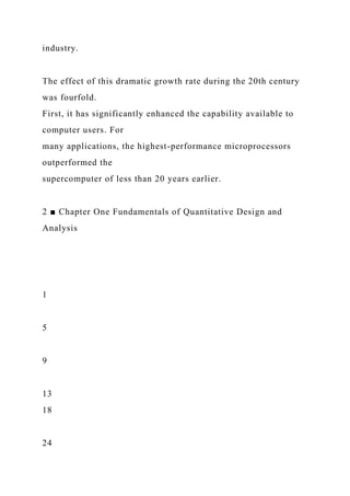
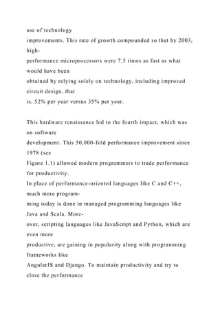
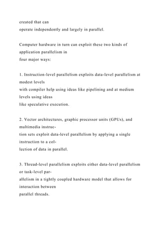
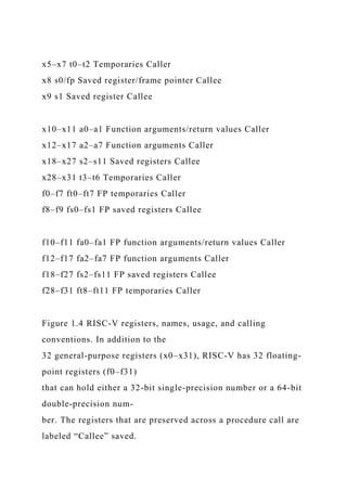
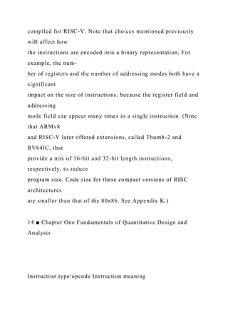
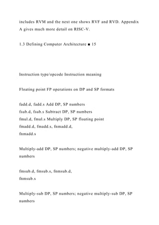
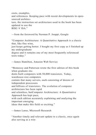
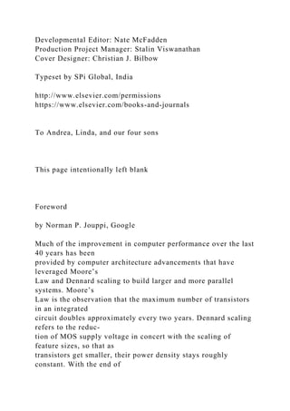
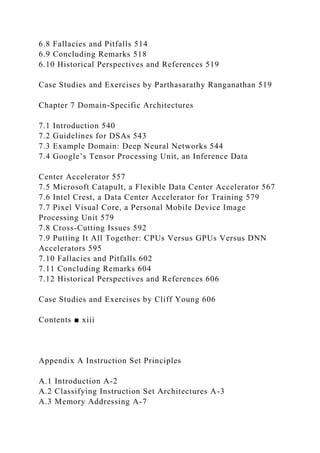
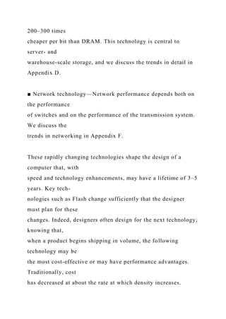
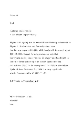
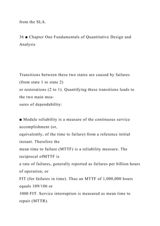
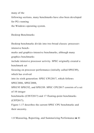
118. opcodeimm [4:0]
imm [4:1|11]
rs1
rs1
rs2
rs2
funct3
funct3
imm [11:5]
opcoderdrs1 funct3imm [11:0]
opcoderdimm [31:12]
J-typeopcoderdimm [20|10:1|11|19:12]

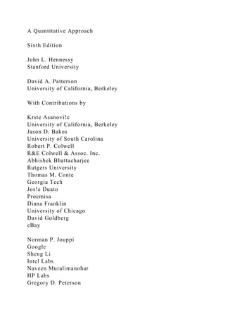
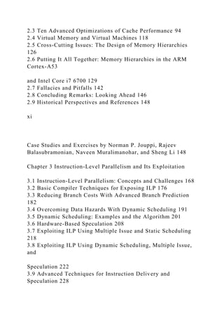
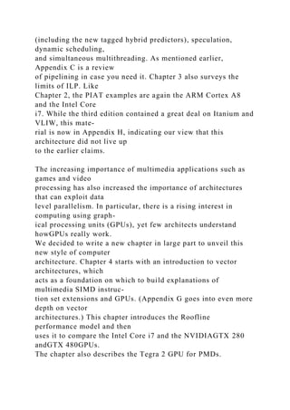
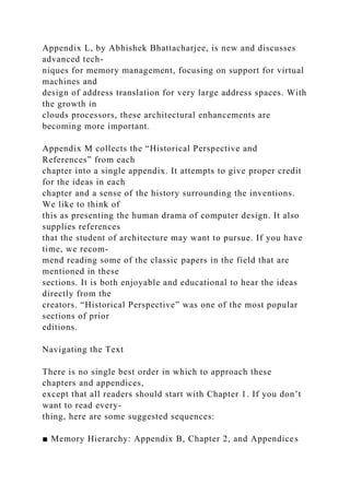
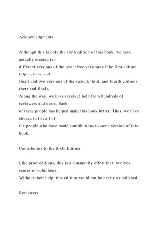
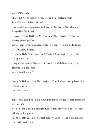
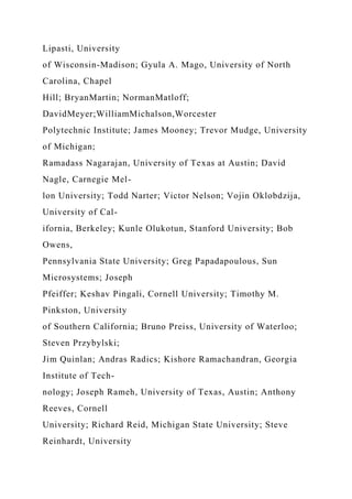
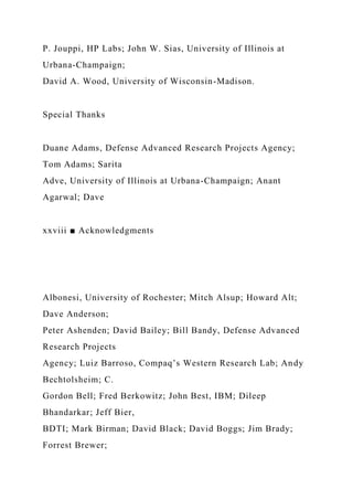
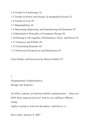
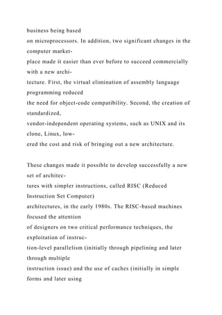
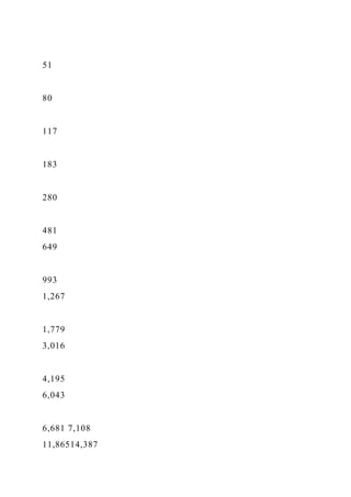
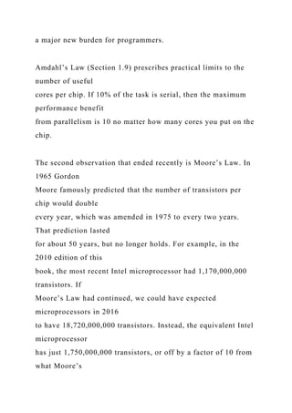
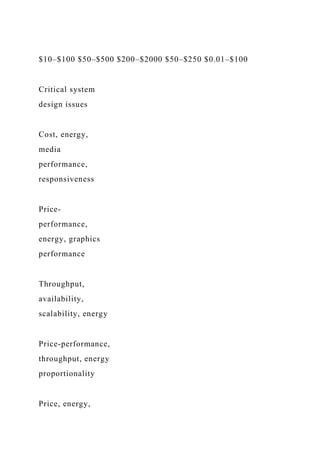
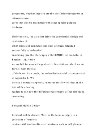
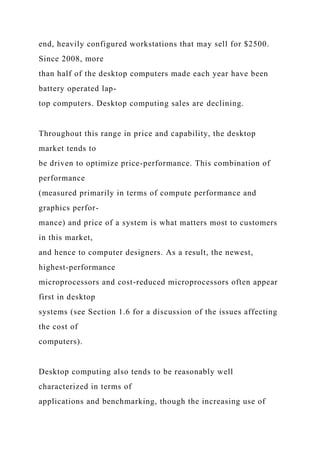
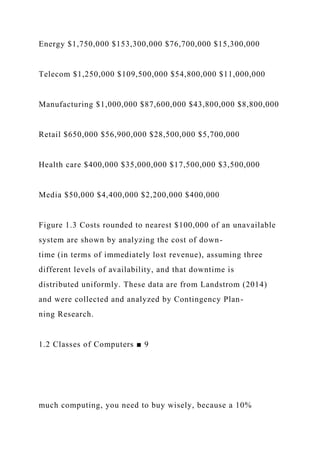
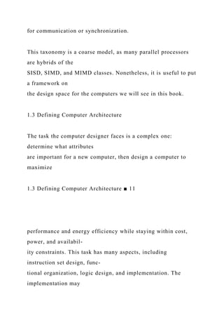
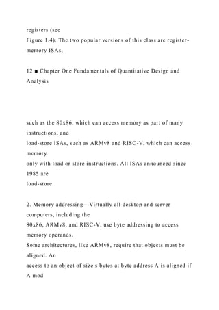
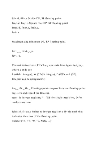
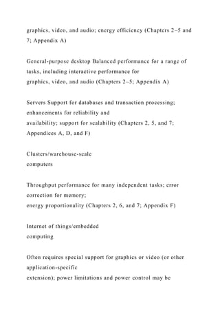
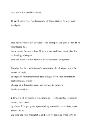
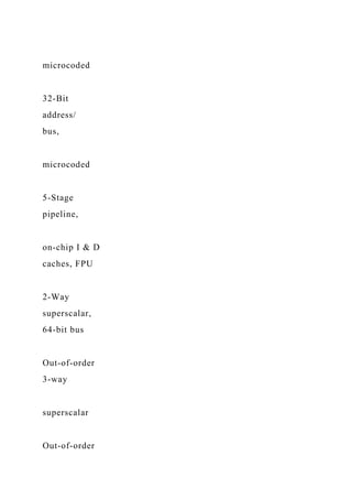
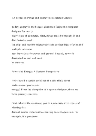
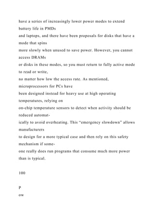
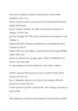
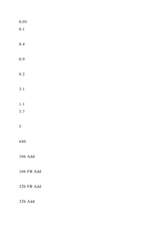
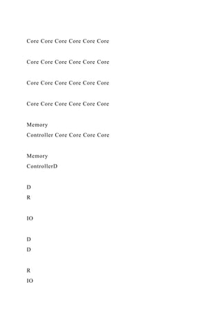
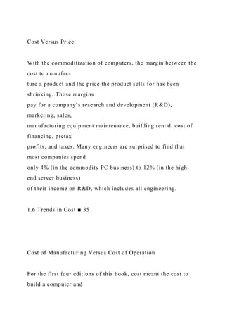
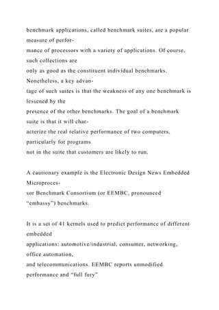
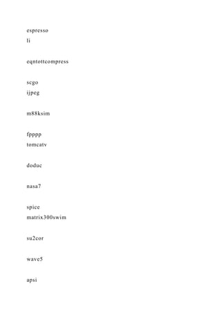
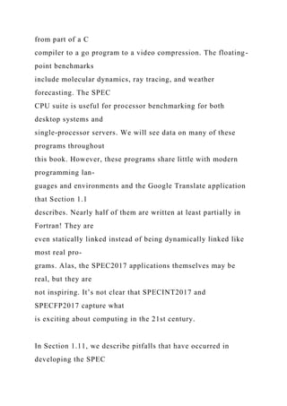
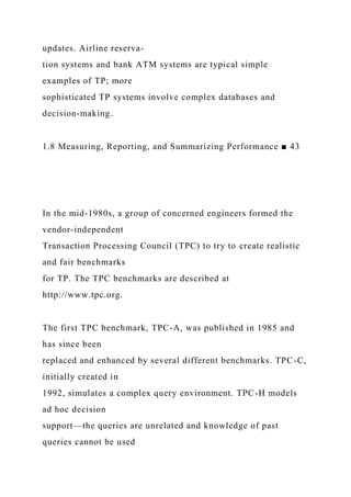
119. B-typeopcodeimm [10:5]imm [12]
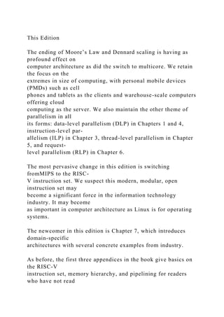
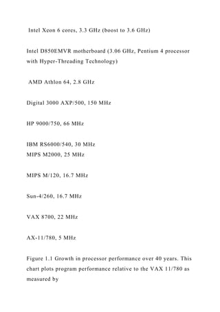
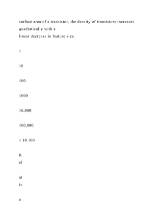
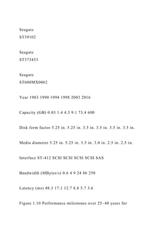
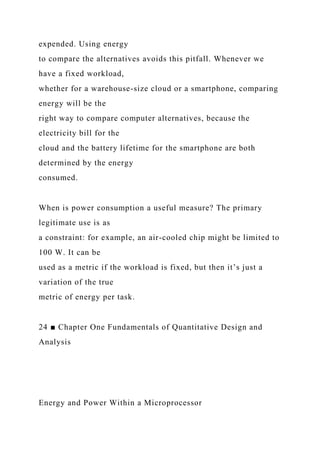
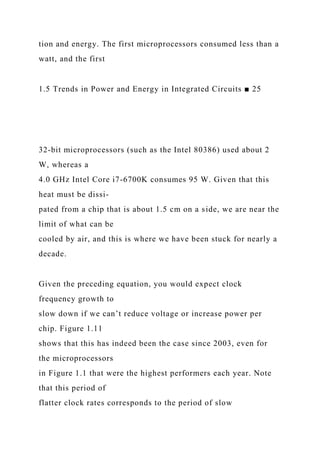
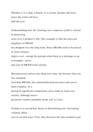
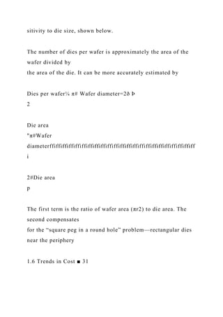
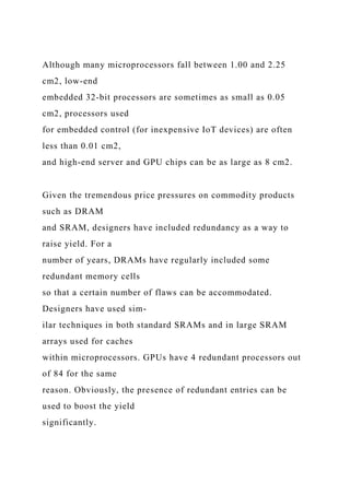
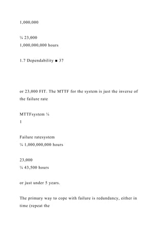
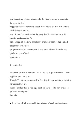
Figure 1.7 The base RISC-V instruction set architecture
formats. All instructions are 32 bits long. The R format is for
integer register-to-register operations, such as ADD, SUB, and
so on. The I format is for loads and immediate oper-
ations, such as LD and ADDI. The B format is for branches and
the J format is for jumps and link. The S format is for
stores. Having a separate format for stores allows the three
register specifiers (rd, rs1, rs2) to always be in the same
location in all formats. The U format is for the wide immediate
instructions (LUI, AUIPC).
16 ■ Chapter One Fundamentals of Quantitative Design and
Analysis
The other challenges facing the computer architect beyond ISA
design are par-
ticularly acute at the present, when the differences among
instruction sets are small
and when there are distinct application areas. Therefore,
starting with the fourth
edition of this book, beyond this quick review, the bulk of the

120. instruction set mate-
rial is found in the appendices (see Appendices A and K).
Genuine Computer Architecture: Designing the Organization
and Hardware to Meet Goals and Functional Requirements
The implementation of a computer has two components:
organization and hard-
ware. The term organization includes the high-level aspects of a
computer’s
design, such as the memory system, the memory interconnect,
and the design of
the internal processor or CPU (central processing unit—where
arithmetic, logic,
branching, and data transfer are implemented). The term
microarchitecture is also
used instead of organization. For example, two processors with
the same instruc-
tion set architectures but different organizations are the
AMDOpteron and the Intel
Core i7. Both processors implement the 80x86 instruction set,
but they have very
different pipeline and cache organizations.
The switch to multiple processors per microprocessor led to the

121. term core also
being used for processors. Instead of saying multiprocessor
microprocessor, the
term multicore caught on. Given that virtually all chips have
multiple processors,
the term central processing unit, or CPU, is fading in
popularity.
Hardware refers to the specifics of a computer, including the
detailed logic
design and the packaging technology of the computer. Often a
line of computers
contains computers with identical instruction set architectures
and very similar
organizations, but they differ in the detailed hardware
implementation. For exam-
ple, the Intel Core i7 (see Chapter 3) and the Intel Xeon E7 (see
Chapter 5) are
nearly identical but offer different clock rates and different
memory systems, mak-
ing the Xeon E7 more effective for server computers.
In this book, the word architecture covers all three aspects of
computer
design—instruction set architecture, organization or

122. microarchitecture, and
hardware.
Computer architects must design a computer to meet functional
requirements
as well as price, power, performance, and availability goals.
Figure 1.8 summarizes
requirements to consider in designing a new computer. Often,
architects also must
determine what the functional requirements are, which can be a
major task. The
requirements may be specific features inspired by the market.
Application software
typically drives the choice of certain functional requirements by
determining how
the computer will be used. If a large body of software exists for
a particular instruc-
tion set architecture, the architect may decide that a new
computer should imple-
ment an existing instruction set. The presence of a large market
for a particular
class of applications might encourage the designers to
incorporate requirements
that would make the computer competitive in that market. Later
chapters examine

123. many of these requirements and features in depth.
1.3 Defining Computer Architecture ■ 17
Architects must also be aware of important trends in both the
technology and
the use of computers because such trends affect not only the
future cost but also the
longevity of an architecture.
1.4 Trends in Technology
If an instruction set architecture is to prevail, it must be
designed to survive rapid
changes in computer technology. After all, a successful new
instruction set
Functional requirements Typical features required or supported
Application area Target of computer
Personal mobile device Real-time performance for a range of
tasks, including interactive performance for

124. graphics, video, and audio; energy efficiency (Chapters 2–5 and
7; Appendix A)
General-purpose desktop Balanced performance for a range of
tasks, including interactive performance for
graphics, video, and audio (Chapters 2–5; Appendix A)
Servers Support for databases and transaction processing;
enhancements for reliability and
availability; support for scalability (Chapters 2, 5, and 7;
Appendices A, D, and F)
Clusters/warehouse-scale
computers
Throughput performance for many independent tasks; error
correction for memory;
energy proportionality (Chapters 2, 6, and 7; Appendix F)
Internet of things/embedded
computing
Often requires special support for graphics or video (or other
application-specific
extension); power limitations and power control may be

125. required; real-time constraints
(Chapters 2, 3, 5, and 7; Appendices A and E)
Level of software compatibility Determines amount of existing
software for computer
At programming language Most flexible for designer; need new
compiler (Chapters 3, 5, and 7; Appendix A)
Object code or binary
compatible
Instruction set architecture is completely defined—little
flexibility—but no investment
needed in software or porting programs (Appendix A)
Operating system requirements Necessary features to support
chosen OS (Chapter 2; Appendix B)
Size of address space Very important feature (Chapter 2); may
limit applications
Memory management Required for modern OS; may be paged or
segmented (Chapter 2)

126. Protection Different OS and application needs: page versus
segment; virtual machines (Chapter 2)
Standards Certain standards may be required by marketplace
Floating point Format and arithmetic: IEEE 754 standard
(Appendix J), special arithmetic for graphics
or signal processing
I/O interfaces For I/O devices: Serial ATA, Serial Attached
SCSI, PCI Express (Appendices D and F)
Operating systems UNIX, Windows, Linux, CISCO IOS
Networks Support required for different networks: Ethernet,
Infiniband (Appendix F)
Programming languages Languages (ANSI C, C++, Java,
Fortran) affect instruction set (Appendix A)
Figure 1.8 Summary of some of the most important functional
requirements an architect faces. The left-hand
column describes the class of requirement, while the right-hand
column gives specific examples. The right-hand col-
umn also contains references to chapters and appendices that

127. deal with the specific issues.
18 ■ Chapter One Fundamentals of Quantitative Design and
Analysis
architecture may last decades—for example, the core of the IBM
mainframe has
been in use for more than 50 years. An architect must plan for
technology changes
that can increase the lifetime of a successful computer.
To plan for the evolution of a computer, the designer must be
aware of rapid
changes in implementation technology. Five implementation
technologies, which
change at a dramatic pace, are critical to modern
implementations:
■ Integrated circuit logic technology—Historically, transistor
density increased
by about 35% per year, quadrupling somewhat over four years.
Increases in
die size are less predictable and slower, ranging from 10% to

128. 20% per year.
The combined effect was a traditional growth rate in transistor
count on a chip
of about 40%–55% per year, or doubling every 18–24 months.
This trend is
popularly known as Moore’s Law. Device speed scales more
slowly, as we
discuss below. Shockingly, Moore’s Law is no more. The
number of devices
per chip is still increasing, but at a decelerating rate. Unlike in
the Moore’s
Law era, we expect the doubling time to be stretched with each
new technol-
ogy generation.
■ Semiconductor DRAM (dynamic random-access memory)—
This technology
is the foundation of main memory, and we discuss it in Chapter
2. The growth
of DRAM has slowed dramatically, from quadrupling every
three years as in
the past. The 8-gigabit DRAM was shipping in 2014, but the 16-
gigabit
DRAM won’t reach that state until 2019, and it looks like there
will be no

129. 32-gigabit DRAM (Kim, 2005). Chapter 2 mentions several
other technologies
that may replace DRAM when it hits its capacity wall.
■ Semiconductor Flash (electrically erasable programmable
read-only mem-
ory)—This nonvolatile semiconductor memory is the standard
storage device
in PMDs, and its rapidly increasing popularity has fueled its
rapid growth
rate in capacity. In recent years, the capacity per Flash chip
increased by about
50%–60% per year, doubling roughly every 2 years. Currently,
Flash
memory is 8–10 times cheaper per bit than DRAM. Chapter 2
describes Flash
memory.
■ Magnetic disk technology—Prior to 1990, density increased
by about 30% per
year, doubling in three years. It rose to 60% per year thereafter,
and increased to
100% per year in 1996. Between 2004 and 2011, it dropped
back to about 40%
per year, or doubled every two years. Recently, disk

130. improvement has slowed
to less than 5% per year. One way to increase disk capacity is to
add more plat-
ters at the same areal density, but there are already seven
platters within the
one-inch depth of the 3.5-inch form factor disks. There is room
for at most
one or twomore platters. The last hope for real density increase
is to use a small
laser on each disk read-write head to heat a 30 nm spot to 400°C
so that it can
be written magnetically before it cools. It is unclear whether
Heat Assisted
Magnetic Recording can be manufactured economically and
reliably, although
Seagate announced plans to ship HAMR in limited production in
2018. HAMR
is the last chance for continued improvement in areal density of
hard disk
1.4 Trends in Technology ■ 19
drives, which are now 8–10 times cheaper per bit than Flash and

131. 200–300 times
cheaper per bit than DRAM. This technology is central to
server- and
warehouse-scale storage, and we discuss the trends in detail in
Appendix D.
■ Network technology—Network performance depends both on
the performance
of switches and on the performance of the transmission system.
We discuss the
trends in networking in Appendix F.
These rapidly changing technologies shape the design of a
computer that, with
speed and technology enhancements, may have a lifetime of 3–5
years. Key tech-
nologies such as Flash change sufficiently that the designer
must plan for these
changes. Indeed, designers often design for the next technology,
knowing that,
when a product begins shipping in volume, the following
technology may be
the most cost-effective or may have performance advantages.
Traditionally, cost
has decreased at about the rate at which density increases.

132. Although technology improves continuously, the impact of these
increases can
be in discrete leaps, as a threshold that allows a new capability
is reached. For
example, when MOS technology reached a point in the early
1980s where between
25,000 and 50,000 transistors could fit on a single chip, it
became possible to build
a single-chip, 32-bit microprocessor. By the late 1980s, first-
level caches could go
on a chip. By eliminating chip crossings within the processor
and between the pro-
cessor and the cache, a dramatic improvement in cost-
performance and energy-
performance was possible. This design was simply unfeasible
until the technology
reached a certain point. With multicore microprocessors and
increasing numbers of
cores each generation, even server computers are increasingly
headed toward a sin-
gle chip for all processors. Such technology thresholds are not
rare and have a sig-
nificant impact on a wide variety of design decisions.

133. Performance Trends: Bandwidth Over Latency
Aswe shall see in Section 1.8, bandwidth or throughput is the
total amount of work
done in a given time, such as megabytes per second for a disk
transfer. In contrast,
latency or response time is the time between the start and the
completion of an
event, such as milliseconds for a disk access. Figure 1.9 plots
the relative improve-
ment in bandwidth and latency for technology milestones for
microprocessors,
memory, networks, and disks. Figure 1.10 describes the
examples and milestones
in more detail.
Performance is the primary differentiator for microprocessors
and networks, so
they have seen the greatest gains: 32,000–40,000# in bandwidth
and 50–90# in
latency. Capacity is generally more important than performance
for memory and
disks, so capacity has improved more, yet bandwidth advances
of 400–2400# are
still much greater than gains in latency of 8–9#.

134. Clearly, bandwidthhasoutpaced latencyacross these technologies
andwill likely
continue to do so. A simple rule of thumb is that bandwidth
grows by at least the
square of the improvement in latency. Computer designers
should plan accordingly.
20 ■ Chapter One Fundamentals of Quantitative Design and
Analysis
Scaling of Transistor Performance and Wires
Integrated circuit processes are characterized by the feature
size, which is the min-
imum size of a transistor or a wire in either the x or y
dimension. Feature sizes
decreased from 10 μm in 1971 to 0.016 μm in 2017; in fact, we
have switched
units, so production in 2017 is referred to as “16 nm,” and 7 nm
chips are under-
way. Since the transistor count per square millimeter of silicon
is determined by the

135. surface area of a transistor, the density of transistors increases
quadratically with a
linear decrease in feature size.
1
10
100
1000
10,000
100,000
1 10 100
R
el
at
iv
e

136. b
an
d
w
id
th
im
p
ro
ve
m
en
t
Relative Latency Improvement
Microprocessor
Memory

137. Network
Disk
(Latency improvement
= Bandwidth improvement)
Figure 1.9 Log-log plot of bandwidth and latency milestones in
Figure 1.10 relative to the first milestone. Note
that latency improved 8–91#, while bandwidth improved about
400–32,000#. Except for networking, we note that
there were modest improvements in latency and bandwidth in
the other three technologies in the six years since the
last edition: 0%–23% in latency and 23%–70% in bandwidth.
Updated from Patterson, D., 2004. Latency lags band-
width. Commun. ACM 47 (10), 71–75.
1.4 Trends in Technology ■ 21
Microprocessor 16-Bit
address/
bus,

138. microcoded
32-Bit
address/
bus,
microcoded
5-Stage
pipeline,
on-chip I & D
caches, FPU
2-Way
superscalar,
64-bit bus
Out-of-order
3-way
superscalar
Out-of-order

139. superpipelined,
on-chip L2
cache
Multicore
OOO 4-way
on chip L3
cache, Turbo
Product Intel 80286 Intel 80386 Intel 80486 Intel Pentium Intel
Pentium Pro Intel Pentium 4 Intel Core i7
Year 1982 1985 1989 1993 1997 2001 2015
Die size (mm2) 47 43 81 90 308 217 122
Transistors 134,000 275,000 1,200,000 3,100,000 5,500,000
42,000,000 1,750,000,000
Processors/chip 1 1 1 1 1 1 4
Pins 68 132 168 273 387 423 1400
Latency (clocks) 6 5 5 5 10 22 14

140. Bus width (bits) 16 32 32 64 64 64 196
Clock rate (MHz) 12.5 16 25 66 200 1500 4000
Bandwidth (MIPS) 2 6 25 132 600 4500 64,000
Latency (ns) 320 313 200 76 50 15 4
Memory module DRAM Page mode
DRAM
Fast page
mode DRAM
Fast page
mode DRAM
Synchronous
DRAM
Double data
rate SDRAM
DDR4

141. SDRAM
Module width (bits) 16 16 32 64 64 64 64
Year 1980 1983 1986 1993 1997 2000 2016
Mbits/DRAM chip 0.06 0.25 1 16 64 256 4096
Die size (mm2) 35 45 70 130 170 204 50
Pins/DRAM chip 16 16 18 20 54 66 134
Bandwidth (MBytes/s) 13 40 160 267 640 1600 27,000
Latency (ns) 225 170 125 75 62 52 30
Local area network Ethernet Fast
Ethernet
Gigabit
Ethernet
10 Gigabit
Ethernet

142. 100 Gigabit
Ethernet
400 Gigabit
Ethernet
IEEE standard 802.3 803.3u 802.3ab 802.3ac 802.3ba 802.3bs
Year 1978 1995 1999 2003 2010 2017
Bandwidth (Mbits/seconds) 10 100 1000 10,000 100,000
400,000
Latency (μs) 3000 500 340 190 100 60
Hard disk 3600 RPM 5400 RPM 7200 RPM 10,000 RPM 15,000
RPM 15,000 RPM
Product CDC WrenI
94145-36
Seagate
ST41600
Seagate
ST15150

143. Seagate
ST39102
Seagate
ST373453
Seagate
ST600MX0062
Year 1983 1990 1994 1998 2003 2016
Capacity (GB) 0.03 1.4 4.3 9.1 73.4 600
Disk form factor 5.25 in. 5.25 in. 3.5 in. 3.5 in. 3.5 in. 3.5 in.
Media diameter 5.25 in. 5.25 in. 3.5 in. 3.0 in. 2.5 in. 2.5 in.
Interface ST-412 SCSI SCSI SCSI SCSI SAS
Bandwidth (MBytes/s) 0.6 4 9 24 86 250
Latency (ms) 48.3 17.1 12.7 8.8 5.7 3.6
Figure 1.10 Performance milestones over 25–40 years for

144. microprocessors, memory, networks, and disks. The
microprocessor milestones are several generations of IA-32
processors, going from a 16-bit bus, microcoded 80286 to
a 64-bit bus, multicore, out-of-order execution, superpipelined
Core i7. Memory module milestones go from 16-bit-
wide, plain DRAM to 64-bit-wide double data rate version 3
synchronous DRAM. Ethernet advanced from 10 Mbits/s
to 400 Gbits/s. Disk milestones are based on rotation speed,
improving from 3600 to 15,000 RPM. Each case is best-
case bandwidth, and latency is the time for a simple operation
assuming no contention. Updated from Patterson, D.,
2004. Latency lags bandwidth. Commun. ACM 47 (10), 71–75.
The increase in transistor performance, however, is more
complex. As feature
sizes shrink, devices shrink quadratically in the horizontal
dimension and also
shrink in the vertical dimension. The shrink in the vertical
dimension requires a
reduction in operating voltage to maintain correct operation and
reliability of the
transistors. This combination of scaling factors leads to a
complex interrelationship

145. between transistor performance and process feature size. To a
first approximation, in
the past the transistor performance improved linearly with
decreasing feature size.
The fact that transistor count improvesquadraticallywith a linear
increase in tran-
sistor performance is both the challenge and the opportunity for
which computer
architects were created! In the early days of microprocessors,
the higher rate of
improvement in density was used to move quickly from 4-bit, to
8-bit, to 16-bit,
to 32-bit, to 64-bit microprocessors.More recently, density
improvements have sup-
ported the introduction ofmultiple processors per chip, wider
SIMDunits, andmany
of the innovations in speculative execution and caches found in
Chapters 2–5.
Although transistors generally improve in performance with
decreased feature
size, wires in an integrated circuit do not. In particular, the
signal delay for a wire
increases in proportion to the product of its resistance and

146. capacitance. Of course,
as feature size shrinks, wires get shorter, but the resistance and
capacitance per unit
length get worse. This relationship is complex, since both
resistance and capaci-
tance depend on detailed aspects of the process, the geometry of
a wire, the loading
on a wire, and even the adjacency to other structures. There are
occasional process
enhancements, such as the introduction of copper, which
provide one-time
improvements in wire delay.
In general, however, wire delay scales poorly compared to
transistor perfor-
mance, creating additional challenges for the designer. In
addition to the power
dissipation limit, wire delay has become a major design obstacle
for large inte-
grated circuits and is often more critical than transistor
switching delay. Larger
and larger fractions of the clock cycle have been consumed by
the propagation
delay of signals on wires, but power now plays an even greater
role than wire delay.

147. 1.5 Trends in Power and Energy in Integrated Circuits
Today, energy is the biggest challenge facing the computer
designer for nearly
every class of computer. First, power must be brought in and
distributed around
the chip, and modern microprocessors use hundreds of pins and
multiple intercon-
nect layers just for power and ground. Second, power is
dissipated as heat and must
be removed.
Power and Energy: A Systems Perspective
How should a system architect or a user think about
performance, power, and
energy? From the viewpoint of a system designer, there are
three primary concerns.
First, what is the maximum power a processor ever requires?
Meeting this
demand can be important to ensuring correct operation. For
example, if a processor

148. 1.5 Trends in Power and Energy in Integrated Circuits ■ 23
attempts to draw more power than a power-supply system can
provide (by drawing
more current than the system can supply), the result is typically
a voltage drop,
which can cause devices to malfunction. Modern processors can
vary widely in
power consumption with high peak currents; hence they provide
voltage indexing
methods that allow the processor to slow down and regulate
voltage within a wider
margin. Obviously, doing so decreases performance.
Second, what is the sustained power consumption? This metric
is widely called
the thermal design power (TDP) because it determines the
cooling requirement.
TDP is neither peak power, which is often 1.5 times higher, nor
is it the actual aver-
age power that will be consumed during a given computation,
which is likely to be
lower still. A typical power supply for a system is typically

149. sized to exceed the
TDP, and a cooling system is usually designed to match or
exceed TDP. Failure
to provide adequate cooling will allow the junction temperature
in the processor to
exceed its maximum value, resulting in device failure and
possibly permanent
damage. Modern processors provide two features to assist in
managing heat, since
the highest power (and hence heat and temperature rise) can
exceed the long-term
average specified by the TDP. First, as the thermal temperature
approaches the
junction temperature limit, circuitry lowers the clock rate,
thereby reducing power.
Should this technique not be successful, a second thermal
overload trap is activated
to power down the chip.
The third factor that designers and users need to consider is
energy and energy
efficiency. Recall that power is simply energy per unit time: 1
watt¼1 joule per
second. Which metric is the right one for comparing processors:
energy or power?

150. In general, energy is always a better metric because it is tied to
a specific task and
the time required for that task. In particular, the energy to
complete a workload is
equal to the average power times the execution time for the
workload.
Thus, if we want to know which of two processors is more
efficient for a given
task, we need to compare energy consumption (not power) for
executing the task.
For example, processor A may have a 20% higher average
power consumption
than processor B, but if A executes the task in only 70% of the
time needed by
B, its energy consumption will be 1.2#0.7¼0.84, which is
clearly better.
One might argue that in a large server or cloud, it is sufficient
to consider the
average power, since the workload is often assumed to be
infinite, but this is mis-
leading. If our cloud were populated with processor Bs rather
than As, then the
cloud would do less work for the same amount of energy

151. expended. Using energy
to compare the alternatives avoids this pitfall. Whenever we
have a fixed workload,
whether for a warehouse-size cloud or a smartphone, comparing
energy will be the
right way to compare computer alternatives, because the
electricity bill for the
cloud and the battery lifetime for the smartphone are both
determined by the energy
consumed.
When is power consumption a useful measure? The primary
legitimate use is as
a constraint: for example, an air-cooled chip might be limited to
100 W. It can be
used as a metric if the workload is fixed, but then it’s just a
variation of the true
metric of energy per task.
24 ■ Chapter One Fundamentals of Quantitative Design and
Analysis
Energy and Power Within a Microprocessor

152. For CMOS chips, the traditional primary energy consumption
has been in switch-
ing transistors, also called dynamic energy. The energy required
per transistor is
proportional to the product of the capacitive load driven by the
transistor and
the square of the voltage:
Energydynamic / Capacitive load#Voltage2
This equation is the energy of pulse of the logic transition of
0!1!0 or
1!0!1. The energy of a single transition (0!1 or 1!0) is then:
Energydynamic / 1=2#Capacitive load#Voltage2
The power required per transistor is just the product of the
energy of a transition
multiplied by the frequency of transitions:
Powerdynamic / 1=2#Capacitive load#Voltage2#Frequency
switched
For a fixed task, slowing clock rate reduces power, but not

153. energy.
Clearly, dynamic power and energy are greatly reduced by
lowering the volt-
age, so voltages have dropped from 5 V to just under 1 V in 20
years. The capac-
itive load is a function of the number of transistors connected to
an output and the
technology, which determines the capacitance of the wires and
the transistors.
Example Some microprocessors today are designed to have
adjustable voltage, so a 15%
reduction in voltage may result in a 15% reduction in frequency.
What would
be the impact on dynamic energy and on dynamic power?
Answer Because the capacitance is unchanged, the answer for
energy is the ratio of the
voltages
Energynew
Energyold
¼ Voltage#0:85ð Þ

154. 2
Voltage2
¼ 0:852 ¼ 0:72
which reduces energy to about 72% of the original. For power,
we add the ratio of
the frequencies
Powernew
Powerold
¼ 0:72# Frequency switched#0:85ð Þ
Frequency switched
¼ 0:61
shrinking power to about 61% of the original.
As we move from one process to the next, the increase in the
number of tran-
sistors switching and the frequency with which they change
dominate the decrease
in load capacitance and voltage, leading to an overall growth in
power consump-

155. tion and energy. The first microprocessors consumed less than a
watt, and the first
1.5 Trends in Power and Energy in Integrated Circuits ■ 25
32-bit microprocessors (such as the Intel 80386) used about 2
W, whereas a
4.0 GHz Intel Core i7-6700K consumes 95 W. Given that this
heat must be dissi-
pated from a chip that is about 1.5 cm on a side, we are near the
limit of what can be
cooled by air, and this is where we have been stuck for nearly a
decade.
Given the preceding equation, you would expect clock
frequency growth to
slow down if we can’t reduce voltage or increase power per
chip. Figure 1.11
shows that this has indeed been the case since 2003, even for
the microprocessors
in Figure 1.1 that were the highest performers each year. Note
that this period of
flatter clock rates corresponds to the period of slow

156. performance improvement
range in Figure 1.1.
Distributing the power, removing the heat, and preventing hot
spots have
become increasingly difficult challenges. Energy is now the
major constraint to
using transistors; in the past, it was the raw silicon area.
Therefore modern
1
10
100
1000
10,000
19
78
19
80

157. 19
82
19
84
19
86
19
88
19
90
19
92
19
94
19
96

158. 19
98
20
00
20
02
20
04
20
06
20
08
20
10
20
12
20

159. 14
20
16
20
18
C
lo
ck
r
at
e
(M
H
z)
Intel Pentium4 Xeon
3200 MHz in 2003

160. Intel Skylake Core i7
4200 MHz in 2017
Intel Pentium III
1000 MHz in 2000
Digital Alpha 21164A
500 MHz in 1996
Digital Alpha 21064
150 MHz in 1992
MIPS M2000
25 MHz in 1989
Digital VAX-11/780
5 MHz in 1978
Sun-4 SPARC
16.7 MHz in 1986
15%/year
40%/year

161. 2%/year
Figure 1.11 Growth in clock rate ofmicroprocessors in Figure
1.1. Between 1978 and 1986, the clock rate improved
less than 15% per year while performance improved by 22% per
year. During the “renaissance period” of 52% per-
formance improvement per year between 1986 and 2003, clock
rates shot up almost 40% per year. Since then, the
clock rate has been nearly flat, growing at less than 2% per
year, while single processor performance improved
recently at just 3.5% per year.
26 ■ Chapter One Fundamentals of Quantitative Design and
Analysis
microprocessors offer many techniques to try to improve energy
efficiency despite
flat clock rates and constant supply voltages:
1. Do nothing well. Most microprocessors today turn off the
clock of inactive
modules to save energy and dynamic power. For example, if no
floating-point

162. instructions are executing, the clock of the floating-point unit is
disabled. If
some cores are idle, their clocks are stopped.
2. Dynamic voltage-frequency scaling (DVFS). The second
technique comes
directly from the preceding formulas. PMDs, laptops, and even
servers have
periods of low activity where there is no need to operate at the
highest clock
frequency and voltages. Modern microprocessors typically offer
a few clock
frequencies and voltages in which to operate that use lower
power and energy.
Figure 1.12 plots the potential power savings via DVFS for a
server as the work-
load shrinks for three different clock rates: 2.4, 1.8, and 1 GHz.
The overall
server power savings is about 10%–15% for each of the two
steps.
3. Design for the typical case. Given that PMDs and laptops are
often idle, mem-
ory and storage offer low power modes to save energy. For
example, DRAMs

163. have a series of increasingly lower power modes to extend
battery life in PMDs
and laptops, and there have been proposals for disks that have a
mode that spins
more slowly when unused to save power. However, you cannot
access DRAMs
or disks in these modes, so you must return to fully active mode
to read or write,
no matter how low the access rate. As mentioned,
microprocessors for PCs have
been designed instead for heavy use at high operating
temperatures, relying on
on-chip temperature sensors to detect when activity should be
reduced automat-
ically to avoid overheating. This “emergency slowdown” allows
manufacturers
to design for a more typical case and then rely on this safety
mechanism if some-
one really does run programs that consume much more power
than is typical.
100
P
ow

164. er
(
%
o
f p
ea
k)
80
60
40
20
0
1 GHz
DVS savings (%)

165. 1.8 GHz
2.4 GHz
Idle 7 14 21 29 36 43 50 57 64 71 79 86 93 100
Compute load (%)
Figure 1.12 Energy savings for a server using an AMD Opteron
microprocessor, 8 GB
of DRAM, and one ATA disk. At 1.8 GHz, the server can handle
at most up to two-thirds
of the workload without causing service-level violations, and at
1 GHz, it can safely han-
dle only one-third of the workload (Figure 5.11 in Barroso and
H€olzle, 2009).
1.5 Trends in Power and Energy in Integrated Circuits ■ 27
4. Overclocking. Intel started offering Turbo mode in 2008,
where the chip decides
that it is safe to run at a higher clock rate for a short time,
possibly on just a few
cores, until temperature starts to rise. For example, the 3.3 GHz
Core i7 can run

166. in short bursts for 3.6 GHz. Indeed, the highest-performing
microprocessors
each year since 2008 shown in Figure 1.1 have all offered
temporary overclock-
ing of about 10% over the nominal clock rate. For single-
threaded code, these
microprocessors can turn off all cores but one and run it faster.
Note that,
although the operating system can turn off Turbo mode, there is
no notification
once it is enabled, so the programmers may be surprised to see
their programs
vary in performance because of room temperature!
Although dynamic power is traditionally thought of as the
primary source of
power dissipation in CMOS, static power is becoming an
important issue because
leakage current flows even when a transistor is off:
Powerstatic / Currentstatic#Voltage
That is, static power is proportional to the number of devices.
Thus increasing the number of transistors increases power even
if they are idle,

167. and current leakage increases in processors with smaller
transistor sizes. As a
result, very low-power systems are even turning off the power
supply (power gat-
ing) to inactive modules in order to control loss because of
leakage. In 2011 the
goal for leakage was 25% of the total power consumption, with
leakage in
high-performance designs sometimes far exceeding that goal.
Leakage can be as
high as 50% for such chips, in part because of the large SRAM
caches that need
power to maintain the storage values. (The S in SRAM is for
static.) The only hope
to stop leakage is to turn off power to the chips’ subsets.
Finally, because the processor is just a portion of the whole
energy cost of a sys-
tem, it canmake sense to use a faster, less energy-efficient
processor to allow the rest
of the system to go into a sleep mode. This strategy is known as
race-to-halt.
The importance of power and energy has increased the scrutiny

168. on the effi-
ciency of an innovation, so the primary evaluation now is tasks
per joule or per-
formance per watt, contrary to performance per mm2 of silicon
as in the past. This
new metric affects approaches to parallelism, as we will see in
Chapters 4 and 5.
The Shift in Computer Architecture Because of Limits of
Energy
As transistor improvement decelerates, computer architects
must look elsewhere
for improved energy efficiency. Indeed, given the energy
budget, it is easy today
to design a microprocessor with so many transistors that they
cannot all be turned
on at the same time. This phenomenon has been called dark
silicon, in that much of
a chip cannot be unused (“dark”) at any moment in time because
of thermal con-
straints. This observation has led architects to reexamine the
fundamentals of pro-
cessors’ design in the search for a greater energy-cost
performance.

169. Figure 1.13, which lists the energy cost and area cost of the
building blocks of
a modern computer, reveals surprisingly large ratios. For
example, a 32-bit
28 ■ Chapter One Fundamentals of Quantitative Design and
Analysis
floating-point addition uses 30 times as much energy as an 8-bit
integer add. The
area difference is even larger, by 60 times. However, the
biggest difference is in
memory; a 32-bit DRAM access takes 20,000 times as much
energy as an 8-bit
addition. A small SRAM is 125 times more energy-efficient
than DRAM, which
demonstrates the importance of careful uses of caches and
memory buffers.
The new design principle of minimizing energy per task
combined with the
relative energy and area costs in Figure 1.13 have inspired a

170. new direction for com-
puter architecture, which we describe in Chapter 7. Domain-
specific processors
save energy by reducing wide floating-point operations and
deploying special-pur-
pose memories to reduce accesses to DRAM. They use those
saving to provide
10–100 more (narrower) integer arithmetic units than a
traditional processor.
Although such processors perform only a limited set of tasks,
they perform them
remarkably faster and more energy efficiently than a general-
purpose processor.
Like a hospital with general practitioners and medical
specialists, computers in
this energy-aware world will likely be combinations of general-
purpose cores that
can perform any task and special-purpose cores that do a few
things extremely well
and even more cheaply.
1.6 Trends in Cost
Although costs tend to be less important in some computer

171. designs—specifically
supercomputers—cost-sensitive designs are of growing
significance. Indeed, in
the past 35 years, the use of technology improvements to lower
cost, as well as
increase performance, has been a major theme in the computer
industry.
Relative energy cost
1
Energy numbers are from Mark Horowitz *Computing’s Energy
problem (and what we can do about it)*. ISSCC 2014
Area numbers are from synthesized result using Design
compiler under TSMC 45nm tech node. FP units used
DesignWare Library.
10 100 1000 10000 1 10 100 1000
Relative area cost
Operation:
8b Add 0.03

172. 0.05
0.1
0.4
0.9
0.2
3.1
1.1
3.7
5
640
16b Add
16b FB Add
32b FB Add
32b Add

173. 8b Mult
32b Mult
16b FB Mult
32b FB Mult
32b SRAM Read (8KB)
32b DRAM Read
Energy (pJ) Area (µm2)
36
67
137
1360
4184
282

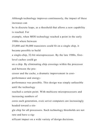
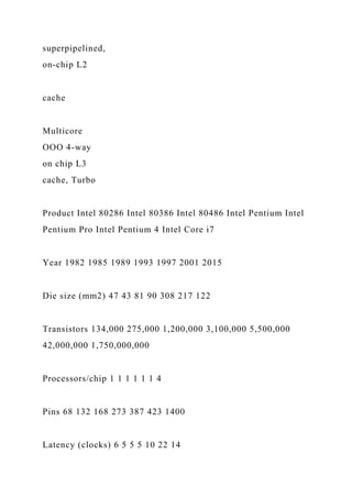
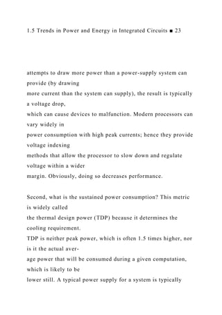
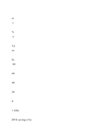
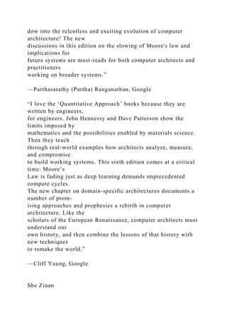
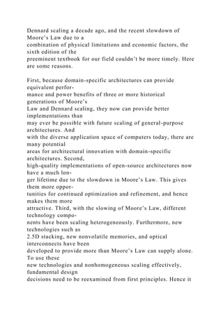
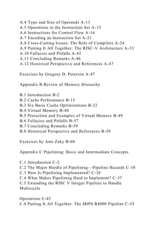
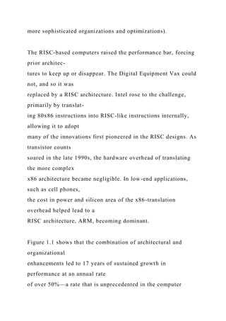
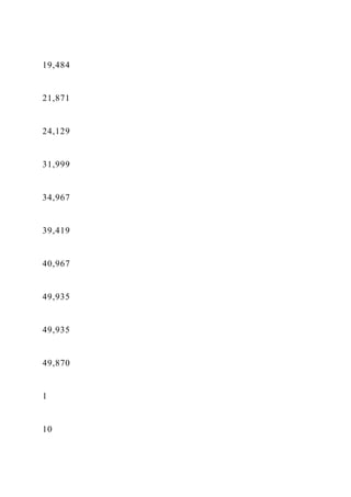
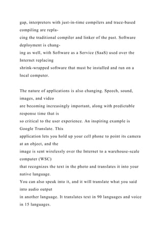
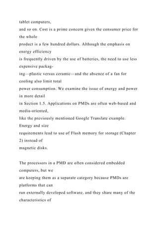
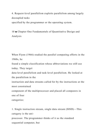
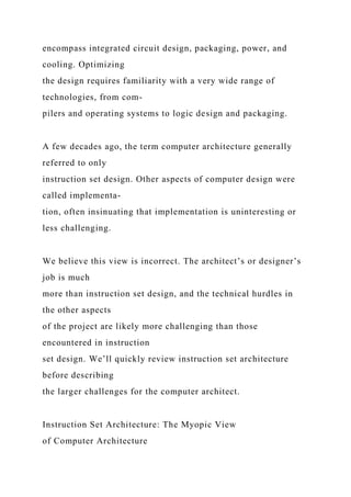
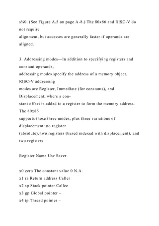
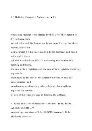
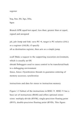
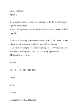
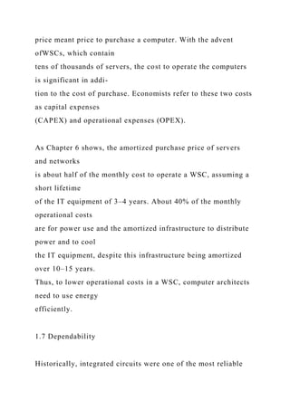
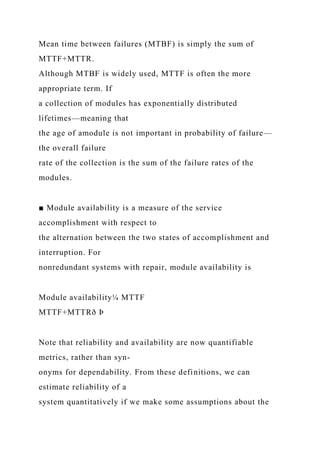
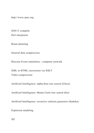
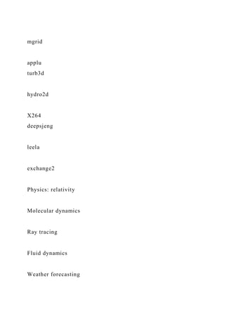
174. 3495
1640
7700
N/A
N/A
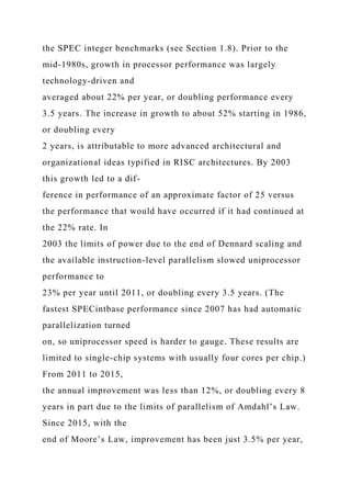
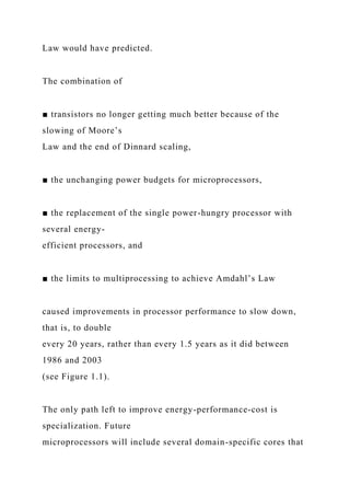
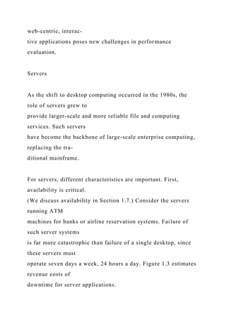
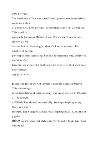
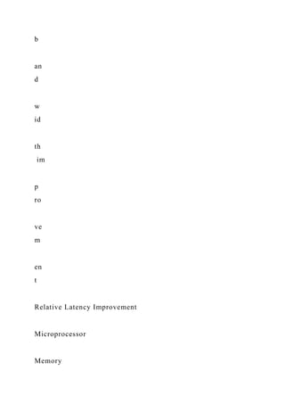
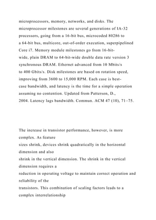
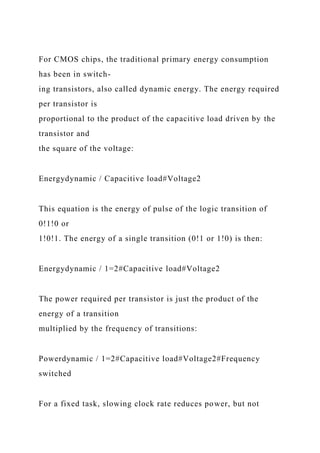
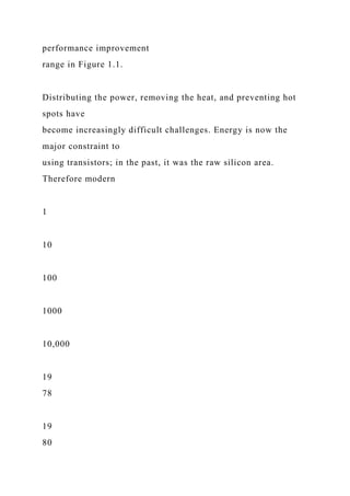
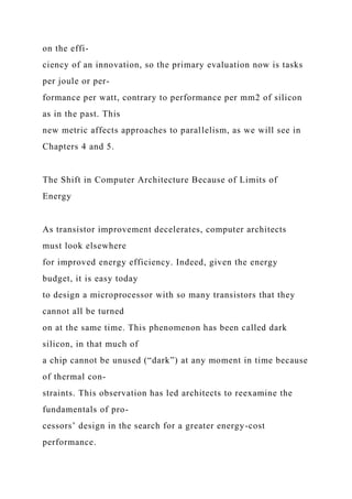
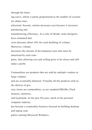
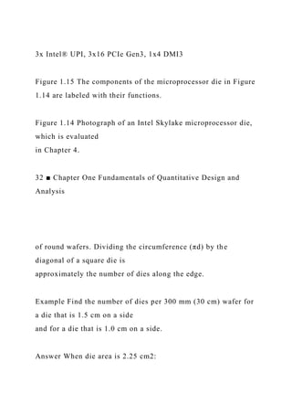
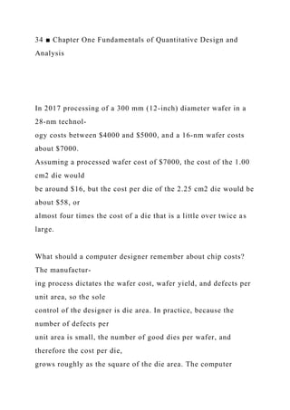
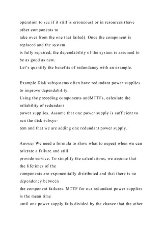
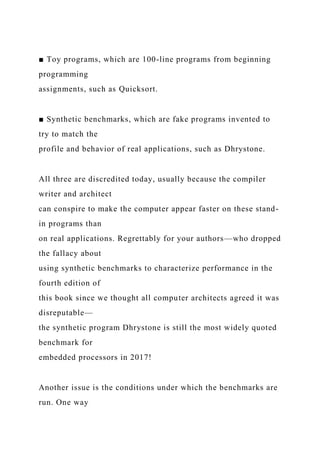
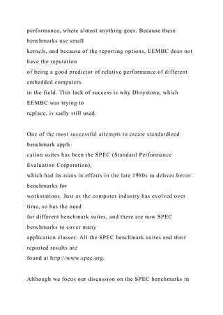
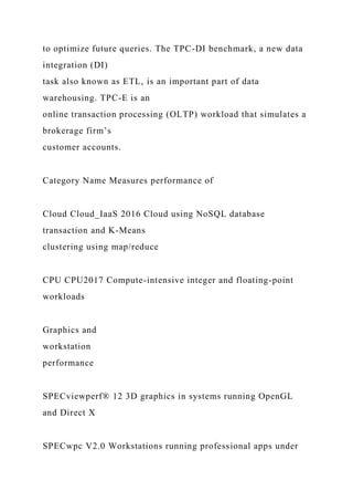
Figure 1.13 Comparison of the energy and die area of arithmetic
operations and energy cost of accesses to SRAM
and DRAM. [Azizi][Dally]. Area is for TSMC 45 nm technology
node.
1.6 Trends in Cost ■ 29
Textbooks often ignore the cost half of cost-performance
because costs change,
thereby dating books, and because the issues are subtle and
differ across industry
segments. Nevertheless, it’s essential for computer architects to

175. have an under-
standing of cost and its factors in order to make intelligent
decisions about whether
a new feature should be included in designs where cost is an
issue. (Imagine archi-
tects designing skyscrapers without any information on costs of
steel beams and
concrete!)
This section discusses the major factors that influence the cost
of a computer
and how these factors are changing over time.
The Impact of Time, Volume, and Commoditization
The cost of a manufactured computer component decreases over
time even without
significant improvements in the basic implementation
technology. The underlying
principle that drives costs down is the learning curve—
manufacturing costs
decrease over time. The learning curve itself is best measured
by change in
yield—the percentage of manufactured devices that survives the
testing procedure.

176. Whether it is a chip, a board, or a system, designs that have
twice the yield will have
half the cost.
Understanding how the learning curve improves yield is critical
to projecting
costs over a product’s life. One example is that the price per
megabyte of DRAM
has dropped over the long term. Since DRAMs tend to be priced
in close relation-
ship to cost—except for periods when there is a shortage or an
oversupply—price
and cost of DRAM track closely.
Microprocessor prices also drop over time, but because they are
less standard-
ized than DRAMs, the relationship between price and cost is
more complex. In a
period of significant competition, price tends to track cost
closely, although micro-
processor vendors probably rarely sell at a loss.
Volume is a second key factor in determining cost. Increasing
volumes affect
cost in several ways. First, they decrease the time needed to get

177. through the learn-
ing curve, which is partly proportional to the number of systems
(or chips) man-
ufactured. Second, volume decreases cost because it increases
purchasing and
manufacturing efficiency. As a rule of thumb, some designers
have estimated that
costs decrease about 10% for each doubling of volume.
Moreover, volume
decreases the amount of development costs that must be
amortized by each com-
puter, thus allowing cost and selling price to be closer and still
make a profit.
Commodities are products that are sold by multiple vendors in
large volumes
and are essentially identical. Virtually all the products sold on
the shelves of gro-
cery stores are commodities, as are standard DRAMs, Flash
memory, monitors,
and keyboards. In the past 30 years, much of the personal
computer industry
has become a commodity business focused on building desktop
and laptop com-
puters running Microsoft Windows.

178. Because many vendors ship virtually identical products, the
market is highly
competitive. Of course, this competition decreases the gap
between cost and selling
30 ■ Chapter One Fundamentals of Quantitative Design and
Analysis
price, but it also decreases cost. Reductions occur because a
commodity market has
both volume and a clear product definition, which allows
multiple suppliers to
compete in building components for the commodity product. As
a result, the over-
all product cost is lower because of the competition among the
suppliers of the
components and the volume efficiencies the suppliers can
achieve. This rivalry
has led to the low end of the computer business being able to
achieve better
price-performance than other sectors and has yielded greater
growth at the low

179. end, although with very limited profits (as is typical in any
commodity business).
Cost of an Integrated Circuit
Why would a computer architecture book have a section on
integrated circuit
costs? In an increasingly competitive computer marketplace
where standard
parts—disks, Flash memory, DRAMs, and so on—are becoming
a significant por-
tion of any system’s cost, integrated circuit costs are becoming
a greater portion of
the cost that varies between computers, especially in the high-
volume, cost-
sensitive portion of the market. Indeed, with PMDs’ increasing
reliance of whole
systems on a chip (SOC), the cost of the integrated circuits is
much of the cost of the
PMD. Thus computer designers must understand the costs of
chips in order to
understand the costs of current computers.
Although the costs of integrated circuits have dropped
exponentially, the basic

180. process of silicon manufacture is unchanged: A wafer is still
tested and chopped
into dies that are packaged (see Figures 1.14–1.16). Therefore
the cost of a pack-
aged integrated circuit is
Cost of integrated circuit¼Cost of die +Cost of testing die
+Cost of packaging and final test
Final test yield
In this section, we focus on the cost of dies, summarizing the
key issues in testing
and packaging at the end.
Learning how to predict the number of good chips per wafer
requires first learn-
ing howmany dies fit on a wafer and then learning how to
predict the percentage of
those that will work. From there it is simple to predict cost:
Cost of die¼ Cost of wafer
Dies per wafer#Die yield
The most interesting feature of this initial term of the chip cost
equation is its sen-

181. sitivity to die size, shown below.
The number of dies per wafer is approximately the area of the
wafer divided by
the area of the die. It can be more accurately estimated by
Dies per wafer¼ π# Wafer diameter=2ð Þ
2
Die area
"π#Wafer
diameterffiffiffiffiffiffiffiffiffiffiffiffiffiffiffiffiffiffiffiffiffiffiff
i
2#Die area
p
The first term is the ratio of wafer area (πr2) to die area. The
second compensates
for the “square peg in a round hole” problem—rectangular dies
near the periphery
1.6 Trends in Cost ■ 31

182. Core Core Core Core Core Core
Core Core Core Core Core Core
Core Core Core Core Core Core
Core Core Core Core Core Core
Memory
Controller Core Core Core Core
Memory
ControllerD
D
R
IO
D
D
R
IO

183. 3x Intel® UPI, 3x16 PCIe Gen3, 1x4 DMI3
Figure 1.15 The components of the microprocessor die in Figure
1.14 are labeled with their functions.
Figure 1.14 Photograph of an Intel Skylake microprocessor die,
which is evaluated
in Chapter 4.
32 ■ Chapter One Fundamentals of Quantitative Design and
Analysis
of round wafers. Dividing the circumference (πd) by the
diagonal of a square die is
approximately the number of dies along the edge.
Example Find the number of dies per 300 mm (30 cm) wafer for
a die that is 1.5 cm on a side
and for a die that is 1.0 cm on a side.
Answer When die area is 2.25 cm2:

184. Dies per wafer¼ π# 30=2ð Þ
2
2:25
" π#30ffiffiffiffiffiffiffiffiffiffiffiffiffiffiffiffi
2#2:25
p ¼ 706:9
2:25
"94:2
2:12
¼ 270
Because the area of the larger die is 2.25 times bigger, there are
roughly 2.25 as
many smaller dies per wafer:
Dies per wafer¼ π# 30=2ð Þ
2
1:00
" π#30ffiffiffiffiffiffiffiffiffiffiffiffiffiffiffiffi

185. 2#1:00
p ¼ 706:9
1:00
"94:2
1:41
¼ 640
However, this formula gives only the maximum number of dies
per wafer. The
critical question is: What is the fraction of good dies on a
wafer, or the die yield? A
simple model of integrated circuit yield, which assumes that
defects are randomly
Figure 1.16 This 200mmdiameter wafer of RISC-V dies was
designed by SiFive. It has
two types of RISC-V dies using an older, larger processing line.
An FE310 die is 2.65
mm # 2.72 mm and an SiFive test die that is 2.89 mm # 2.72
mm. The wafer contains
1846 of the former and 1866 of the latter, totaling 3712 chips.
1.6 Trends in Cost ■ 33

186. distributed over the wafer and that yield is inversely
proportional to the complexity
of the fabrication process, leads to the following:
Die yield¼Wafer yield#1= 1 +Defects per unit area#Die areað
ÞN
This Bose-Einstein formula is an empirical model developed by
looking at the
yield of many manufacturing lines (Sydow, 2006), and it still
applies today.Wafer
yield accounts for wafers that are completely bad and so need
not be tested. For
simplicity, we’ll just assume the wafer yield is 100%. Defects
per unit area is a
measure of the random manufacturing defects that occur. In
2017 the value was
typically 0.08–0.10 defects per square inch for a 28-nm node
and 0.10–0.30 for
the newer 16 nm node because it depends on the maturity of the
process (recall
the learning curve mentioned earlier). The metric versions are

187. 0.012–0.016 defects
per square centimeter for 28 nm and 0.016–0.047 for 16 nm.
Finally, N is a
parameter called the process-complexity factor, a measure of
manufacturing
difficulty. For 28 nm processes in 2017, N is 7.5–9.5. For a 16
nm process,
N ranges from 10 to 14.
Example Find the die yield for dies that are 1.5 cm on a side
and 1.0 cm on a side, assuming a
defect density of 0.047 per cm2 and N is 12.
Answer The total die areas are 2.25 and 1.00 cm2. For the larger
die, the yield is
Die yield¼ 1= 1 + 0:047#2:25ð Þ12#270¼ 120
For the smaller die, the yield is
Die yield¼ 1= 1 + 0:047#1:00ð Þ12#640¼ 444
The bottom line is the number of good dies per wafer. Less than
half of all the large
dies are good, but nearly 70% of the small dies are good.

188. Although many microprocessors fall between 1.00 and 2.25
cm2, low-end
embedded 32-bit processors are sometimes as small as 0.05
cm2, processors used
for embedded control (for inexpensive IoT devices) are often
less than 0.01 cm2,
and high-end server and GPU chips can be as large as 8 cm2.
Given the tremendous price pressures on commodity products
such as DRAM
and SRAM, designers have included redundancy as a way to
raise yield. For a
number of years, DRAMs have regularly included some
redundant memory cells
so that a certain number of flaws can be accommodated.
Designers have used sim-
ilar techniques in both standard SRAMs and in large SRAM
arrays used for caches
within microprocessors. GPUs have 4 redundant processors out
of 84 for the same
reason. Obviously, the presence of redundant entries can be
used to boost the yield
significantly.

189. 34 ■ Chapter One Fundamentals of Quantitative Design and
Analysis
In 2017 processing of a 300 mm (12-inch) diameter wafer in a
28-nm technol-
ogy costs between $4000 and $5000, and a 16-nm wafer costs
about $7000.
Assuming a processed wafer cost of $7000, the cost of the 1.00
cm2 die would
be around $16, but the cost per die of the 2.25 cm2 die would be
about $58, or
almost four times the cost of a die that is a little over twice as
large.
What should a computer designer remember about chip costs?
The manufactur-
ing process dictates the wafer cost, wafer yield, and defects per
unit area, so the sole
control of the designer is die area. In practice, because the
number of defects per
unit area is small, the number of good dies per wafer, and
therefore the cost per die,
grows roughly as the square of the die area. The computer

190. designer affects die size,
and thus cost, both by what functions are included on or
excluded from the die and
by the number of I/O pins.
Before we have a part that is ready for use in a computer, the
die must be tested
(to separate the good dies from the bad), packaged, and tested
again after packag-
ing. These steps all add significant costs, increasing the total by
half.
The preceding analysis focused on the variable costs of
producing a functional
die, which is appropriate for high-volume integrated circuits.
There is, however,
one very important part of the fixed costs that can significantly
affect the cost
of an integrated circuit for low volumes (less than 1 million
parts), namely, the cost
of a mask set. Each step in the integrated circuit process
requires a separate mask.
Therefore, for modern high-density fabrication processes with
up to 10 metal
layers, mask costs are about $4 million for 16 nm and $1.5

191. million for 28 nm.
The good news is that semiconductor companies offer “shuttle
runs” to dramat-
ically lower the costs of tiny test chips. They lower costs by
putting many small
designs onto a single die to amortize the mask costs, and then
later split the dies
into smaller pieces for each project. Thus TSMC delivers 80–
100 untested dies that
are 1.57#1.57 mm in a 28 nm process for $30,000 in 2017.
Although these die are
tiny, they offer the architect millions of transistors to play with.
For example, sev-
eral RISC-V processors would fit on such a die.
Although shuttle runs help with prototyping and debugging
runs, they don’t
address small-volume production of tens to hundreds of
thousands of parts.
Because mask costs are likely to continue to increase, some
designers are incorpo-
rating reconfigurable logic to enhance the flexibility of a part
and thus reduce the
cost implications of masks.

192. Cost Versus Price
With the commoditization of computers, the margin between the
cost to manufac-
ture a product and the price the product sells for has been
shrinking. Those margins
pay for a company’s research and development (R&D),
marketing, sales,
manufacturing equipment maintenance, building rental, cost of
financing, pretax
profits, and taxes. Many engineers are surprised to find that
most companies spend
only 4% (in the commodity PC business) to 12% (in the high-
end server business)
of their income on R&D, which includes all engineering.
1.6 Trends in Cost ■ 35
Cost of Manufacturing Versus Cost of Operation
For the first four editions of this book, cost meant the cost to
build a computer and

193. price meant price to purchase a computer. With the advent
ofWSCs, which contain
tens of thousands of servers, the cost to operate the computers
is significant in addi-
tion to the cost of purchase. Economists refer to these two costs
as capital expenses
(CAPEX) and operational expenses (OPEX).
As Chapter 6 shows, the amortized purchase price of servers
and networks
is about half of the monthly cost to operate a WSC, assuming a
short lifetime
of the IT equipment of 3–4 years. About 40% of the monthly
operational costs
are for power use and the amortized infrastructure to distribute
power and to cool
the IT equipment, despite this infrastructure being amortized
over 10–15 years.
Thus, to lower operational costs in a WSC, computer architects
need to use energy
efficiently.
1.7 Dependability
Historically, integrated circuits were one of the most reliable

194. components of a com-
puter. Although their pins may be vulnerable, and faults may
occur over commu-
nication channels, the failure rate inside the chip was very low.
That conventional
wisdom is changing as we head to feature sizes of 16 nm and
smaller, because both
transient faults and permanent faults are becoming more
commonplace, so archi-
tects must design systems to cope with these challenges. This
section gives a quick
overview of the issues in dependability, leaving the official
definition of the terms
and approaches to Section D.3 in Appendix D.
Computers are designed and constructed at different layers of
abstraction. We
can descend recursively down through a computer seeing
components enlarge
themselves to full subsystems until we run into individual
transistors. Although
some faults are widespread, like the loss of power, many can be
limited to a single
component in a module. Thus utter failure of a module at one
level may be con-

195. sidered merely a component error in a higher-level module. This
distinction is
helpful in trying to find ways to build dependable computers.
One difficult question is deciding when a system is operating
properly. This
theoretical point became concrete with the popularity of
Internet services. Infra-
structure providers started offering service level agreements
(SLAs) or service
level objectives (SLOs) to guarantee that their networking or
power service would
be dependable. For example, they would pay the customer a
penalty if they did not
meet an agreement of some hours per month. Thus an SLA
could be used to decide
whether the system was up or down.
Systems alternate between two states of service with respect to
an SLA:
1. Service accomplishment, where the service is delivered as
specified.
2. Service interruption, where the delivered service is different

196. from the SLA.
36 ■ Chapter One Fundamentals of Quantitative Design and
Analysis
Transitions between these two states are caused by failures
(from state 1 to state 2)
or restorations (2 to 1). Quantifying these transitions leads to
the two main mea-
sures of dependability:
■ Module reliability is a measure of the continuous service
accomplishment (or,
equivalently, of the time to failure) from a reference initial
instant. Therefore the
mean time to failure (MTTF) is a reliability measure. The
reciprocal ofMTTF is
a rate of failures, generally reported as failures per billion hours
of operation, or
FIT (for failures in time). Thus an MTTF of 1,000,000 hours
equals 109/106 or
1000 FIT. Service interruption is measured as mean time to
repair (MTTR).

197. Mean time between failures (MTBF) is simply the sum of
MTTF+MTTR.
Although MTBF is widely used, MTTF is often the more
appropriate term. If
a collection of modules has exponentially distributed
lifetimes—meaning that
the age of amodule is not important in probability of failure—
the overall failure
rate of the collection is the sum of the failure rates of the
modules.
■ Module availability is a measure of the service
accomplishment with respect to
the alternation between the two states of accomplishment and
interruption. For
nonredundant systems with repair, module availability is
Module availability¼ MTTF
MTTF+MTTRð Þ
Note that reliability and availability are now quantifiable
metrics, rather than syn-
onyms for dependability. From these definitions, we can
estimate reliability of a
system quantitatively if we make some assumptions about the

198. reliability of com-
ponents and that failures are independent.
Example Assume a disk subsystem with the following
components and MTTF:
■ 10 disks, each rated at 1,000,000-hour MTTF
■ 1 ATA controller, 500,000-hour MTTF
■ 1 power supply, 200,000-hour MTTF
■ 1 fan, 200,000-hour MTTF
■ 1 ATA cable, 1,000,000-hour MTTF
Using the simplifying assumptions that the lifetimes are
exponentially distributed
and that failures are independent, compute the MTTF of the
system as a whole.
Answer The sum of the failure rates is
Failure ratesystem ¼ 10#
1

199. 1,000,000
+
1
500,000
+
1
200,000
+
1
200,000
+
1
1,000,000
¼ 10 + 2 + 5 + 5 + 1
1,000,000 hours
¼ 23

200. 1,000,000
¼ 23,000
1,000,000,000 hours
1.7 Dependability ■ 37
or 23,000 FIT. The MTTF for the system is just the inverse of
the failure rate
MTTFsystem ¼
1
Failure ratesystem
¼ 1,000,000,000 hours
23,000
¼ 43,500 hours
or just under 5 years.
The primary way to cope with failure is redundancy, either in
time (repeat the

201. operation to see if it still is erroneous) or in resources (have
other components to
take over from the one that failed). Once the component is
replaced and the system
is fully repaired, the dependability of the system is assumed to
be as good as new.
Let’s quantify the benefits of redundancy with an example.
Example Disk subsystems often have redundant power supplies
to improve dependability.
Using the preceding components andMTTFs, calculate the
reliability of redundant
power supplies. Assume that one power supply is sufficient to
run the disk subsys-
tem and that we are adding one redundant power supply.
Answer We need a formula to show what to expect when we can
tolerate a failure and still
provide service. To simplify the calculations, we assume that
the lifetimes of the
components are exponentially distributed and that there is no
dependency between
the component failures. MTTF for our redundant power supplies
is the mean time
until one power supply fails divided by the chance that the other

202. will fail before the
first one is replaced. Thus, if the chance of a second failure
before repair is small,
then the MTTF of the pair is large.
Since we have two power supplies and independent failures, the
mean time until
one supply fails is MTTFpower supply/2. A good approximation
of the probability of
a second failure is MTTR over the mean time until the other
power supply fails.
Therefore a reasonable approximation for a redundant pair of
power supplies is
MTTFpower supply pair ¼
MTTFpower supply=2
MTTRpower supply
MTTFpower supply
¼
MTTF2power supply=2
MTTRpower supply
¼

203. MTTF2power supply
2#MTTRpower supply
Using the preceding MTTF numbers, if we assume it takes on
average 24 hours for
a human operator to notice that a power supply has failed and to
replace it, the reli-
ability of the fault tolerant pair of power supplies is
MTTFpower supply pair ¼
MTTF2power supply
2#MTTRpower supply
¼ 200,000
2
2#24 ffi 830,000,000
making the pair about 4150 times more reliable than a single
power supply.
Having quantified the cost, power, and dependability of
computer technology, we
are ready to quantify performance.

204. 38 ■ Chapter One Fundamentals of Quantitative Design and
Analysis
1.8 Measuring, Reporting, and Summarizing Performance
When we say one computer is faster than another one is, what
do we mean? The
user of a cell phone may say a computer is faster when a
program runs in less time,
while an Amazon.com administrator may say a computer is
faster when it com-
pletes more transactions per hour. The cell phone user wants to
reduce response
time—the time between the start and the completion of an
event—also referred
to as execution time. The operator of a WSC wants to increase
throughput—the
total amount of work done in a given time.
In comparing design alternatives, we often want to relate the
performance of
two different computers, say, X and Y. The phrase “X is faster

205. than Y” is used
here to mean that the response time or execution time is lower
on X than on Y
for the given task. In particular, “X is n times as fast as Y” will
mean
Execution timeY
Execution timeX
¼ n
Since execution time is the reciprocal of performance, the
following relationship
holds:
n¼Execution timeY
Execution timeX
¼
1
PerformanceY
1
PerformanceX

206. ¼ PerformanceX
PerformanceY
The phrase “the throughput of X is 1.3 times as fast as Y”
signifies here that the
number of tasks completed per unit time on computer X is 1.3
times the number
completed on Y.
Unfortunately, time is not always the metric quoted in
comparing the perfor-
mance of computers. Our position is that the only consistent and
reliable measure
of performance is the execution time of real programs, and that
all proposed alter-
natives to time as the metric or to real programs as the items
measured have even-
tually led to misleading claims or even mistakes in computer
design.
Even execution time can be defined in different ways depending
on what we
count. The most straightforward definition of time is called
wall-clock time,

207. response time, or elapsed time, which is the latency to complete
a task, including
storage accesses, memory accesses, input/output activities,
operating system over-
head—everything. With multiprogramming, the processor works
on another pro-
gram while waiting for I/O and may not necessarily minimize
the elapsed time of
one program. Thus we need a term to consider this activity.
CPU time recognizes
this distinction and means the time the processor is computing,
not including the
time waiting for I/O or running other programs. (Clearly, the
response time seen by
the user is the elapsed time of the program, not the CPU time.)
Computer users who routinely run the same programs would be
the perfect can-
didates to evaluate a new computer. To evaluate a new system,
these users would
simply compare the execution time of their workloads—the
mixture of programs
1.8 Measuring, Reporting, and Summarizing Performance ■ 39

208. and operating system commands that users run on a computer.
Few are in this
happy situation, however. Most must rely on other methods to
evaluate computers,
and often other evaluators, hoping that these methods will
predict performance for
their usage of the new computer. One approach is benchmark
programs, which are
programs that many companies use to establish the relative
performance of their
computers.
Benchmarks
The best choice of benchmarks to measure performance is real
applications, such as
Google Translate mentioned in Section 1.1. Attempts at running
programs that are
much simpler than a real application have led to performance
pitfalls. Examples
include
■ Kernels, which are small, key pieces of real applications.

209. ■ Toy programs, which are 100-line programs from beginning
programming
assignments, such as Quicksort.
■ Synthetic benchmarks, which are fake programs invented to
try to match the
profile and behavior of real applications, such as Dhrystone.
All three are discredited today, usually because the compiler
writer and architect
can conspire to make the computer appear faster on these stand-
in programs than
on real applications. Regrettably for your authors—who dropped
the fallacy about
using synthetic benchmarks to characterize performance in the
fourth edition of
this book since we thought all computer architects agreed it was
disreputable—
the synthetic program Dhrystone is still the most widely quoted
benchmark for
embedded processors in 2017!
Another issue is the conditions under which the benchmarks are
run. One way

210. to improve the performance of a benchmark has been with
benchmark-specific
compiler flags; these flags often caused transformations that
would be illegal on
many programs or would slow down performance on others. To
restrict this pro-
cess and increase the significance of the results, benchmark
developers typically
require the vendor to use one compiler and one set of flags for
all the programs
in the same language (such as C++ or C). In addition to the
question of compiler
flags, another question is whether source code modifications are
allowed. There are
three different approaches to addressing this question:
1. No source code modifications are allowed.
2. Source code modifications are allowed but are essentially
impossible. For
example, database benchmarks rely on standard database
programs that are tens
of millions of lines of code. The database companies are highly
unlikely to make
changes to enhance the performance for one particular

211. computer.
3. Source modifications are allowed, as long as the altered
version produces the
same output.
40 ■ Chapter One Fundamentals of Quantitative Design and
Analysis
Thekey issue that benchmark designers face in deciding to
allowmodification of the
source is whether such modifications will reflect real practice
and provide useful
insight to users, or whether these changes simply reduce the
accuracy of the bench-
marks as predictors of real performance. As we will see in
Chapter 7, domain-
specific architects often follow the third option when creating
processors for
well-defined tasks.
To overcome the danger of placing too many eggs in one basket,
collections of

212. benchmark applications, called benchmark suites, are a popular
measure of perfor-
mance of processors with a variety of applications. Of course,
such collections are
only as good as the constituent individual benchmarks.
Nonetheless, a key advan-
tage of such suites is that the weakness of any one benchmark is
lessened by the
presence of the other benchmarks. The goal of a benchmark
suite is that it will char-
acterize the real relative performance of two computers,
particularly for programs
not in the suite that customers are likely to run.
A cautionary example is the Electronic Design News Embedded
Microproces-
sor Benchmark Consortium (or EEMBC, pronounced
“embassy”) benchmarks.
It is a set of 41 kernels used to predict performance of different
embedded
applications: automotive/industrial, consumer, networking,
office automation,
and telecommunications. EEMBC reports unmodified
performance and “full fury”

213. performance, where almost anything goes. Because these
benchmarks use small
kernels, and because of the reporting options, EEMBC does not
have the reputation
of being a good predictor of relative performance of different
embedded computers
in the field. This lack of success is why Dhrystone, which
EEMBC was trying to
replace, is sadly still used.
One of the most successful attempts to create standardized
benchmark appli-
cation suites has been the SPEC (Standard Performance
Evaluation Corporation),
which had its roots in efforts in the late 1980s to deliver better
benchmarks for
workstations. Just as the computer industry has evolved over
time, so has the need
for different benchmark suites, and there are now SPEC
benchmarks to cover many
application classes. All the SPEC benchmark suites and their
reported results are
found at http://www.spec.org.
Although we focus our discussion on the SPEC benchmarks in

214. many of the
following sections, many benchmarks have also been developed
for PCs running
the Windows operating system.
Desktop Benchmarks
Desktop benchmarks divide into two broad classes: processor-
intensive bench-
marks and graphics-intensive benchmarks, although many
graphics benchmarks
include intensive processor activity. SPEC originally created a
benchmark set
focusing on processor performance (initially called SPEC89),
which has evolved
into its sixth generation: SPEC CPU2017, which follows
SPEC2006, SPEC2000,
SPEC95 SPEC92, and SPEC89. SPEC CPU2017 consists of a set
of 10 integer
benchmarks (CINT2017) and 17 floating-point benchmarks
(CFP2017).
Figure 1.17 describes the current SPEC CPU benchmarks and
their ancestry.
1.8 Measuring, Reporting, and Summarizing Performance ■ 41

215. http://www.spec.org
GNU C compiler
Perl interpreter
Route planning
General data compression
Discrete Event simulation - computer network
XML to HTML conversion via XSLT
Video compression
Artificial Intelligence: alpha-beta tree search (Chess)
Artificial Intelligence: Monte Carlo tree search (Go)
Artificial Intelligence: recursive solution generator (Sudoku)
Explosion modeling
XZ

216. omnetpp
xalancbmk
h264ref
sjeng
gobmk
astar
hmmer
libquantum
bwaves
cactuBSSN
namd
povray
lbm

217. wrf
gamess
wupwise
apply
galgel
mesa
art
equake
facerec
ammp
lucas
fma3d
sixtrack
parest

218. blender
cam4
imagick
nab
fotonik3d
roms
milc
zeusmp
gromacs
leslie3d
dealII
soplex
calculix
GemsFDTD

219. tonto
sphinx3
mcf
bzip2
vortex
gzip
eon
twolf
vortex
vpr
crafty
parser
perl
gcc

220. espresso
li
eqntottcompress
scgo
ijpeg
m88ksim
fpppp
tomcatv
doduc
nasa7
spice
matrix300swim
su2cor
wave5
apsi

221. mgrid
applu
turb3d
hydro2d
X264
deepsjeng
leela
exchange2
Physics: relativity
Molecular dynamics
Ray tracing
Fluid dynamics
Weather forecasting

222. 3D rendering and animation
Atmosphere modeling
Image manipulation
Molecular dynamics
Computational Electromagnetics
Regional ocean modeling
Biomedical imaging: optical tomography with finite elements
SPEC89SPEC95
Benchmark name by SPEC generation
SPEC92SPEC2000SPEC2006SPEC2017
Figure 1.17 SPEC2017 programs and the evolution of the SPEC
benchmarks over time, with integer programs above the line and
floating-
point programs below the line. Of the 10 SPEC2017 integer
programs, 5 are written in C, 4 in C++., and 1 in Fortran. For
the floating-point

223. programs, the split is 3 in Fortran, 2 in C++, 2 in C, and 6 in
mixed C, C++, and Fortran. The figure shows all 82 of the
programs in the 1989,
1992, 1995, 2000, 2006, and 2017 releases. Gcc is the senior
citizen of the group. Only 3 integer programs and 3 floating-
point programs survived
three or more generations. Although a few are carried over from
generation to generation, the version of the program changes
and either the
input or the size of the benchmark is often expanded to increase
its running time and to avoid perturbation inmeasurement or
domination of the
execution time by some factor other than CPU time. The
benchmark descriptions on the left are for SPEC2017 only and
do not apply to earlier
versions. Programs in the same row from different generations
of SPEC are generally not related; for example, fpppp is not a
CFD code like
bwaves.
42
■
C
hapter

224. O
ne
F
undam
entals
of
Q
uantitative
D
esign
and
A
nalysis
SPEC benchmarks are real programs modified to be portable
and to minimize
the effect of I/O on performance. The integer benchmarks vary

225. from part of a C
compiler to a go program to a video compression. The floating-
point benchmarks
include molecular dynamics, ray tracing, and weather
forecasting. The SPEC
CPU suite is useful for processor benchmarking for both
desktop systems and
single-processor servers. We will see data on many of these
programs throughout
this book. However, these programs share little with modern
programming lan-
guages and environments and the Google Translate application
that Section 1.1
describes. Nearly half of them are written at least partially in
Fortran! They are
even statically linked instead of being dynamically linked like
most real pro-
grams. Alas, the SPEC2017 applications themselves may be
real, but they are
not inspiring. It’s not clear that SPECINT2017 and
SPECFP2017 capture what
is exciting about computing in the 21st century.
In Section 1.11, we describe pitfalls that have occurred in
developing the SPEC

226. CPUbenchmark suite, as well as the challenges in maintaining a
useful and pre-
dictive benchmark suite.
SPECCPU2017 is aimed at processor performance, but
SPECoffersmanyother
benchmarks. Figure 1.18 lists the 17 SPEC benchmarks that are
active in 2017.
Server Benchmarks
Just as servers have multiple functions, so are there multiple
types of benchmarks.
The simplest benchmark is perhaps a processor throughput-
oriented benchmark.
SPEC CPU2017 uses the SPEC CPU benchmarks to construct a
simple throughput
benchmark where the processing rate of a multiprocessor can be
measured by run-
ning multiple copies (usually as many as there are processors)
of each SPEC CPU
benchmark and converting the CPU time into a rate. This leads
to a measurement
called the SPECrate, and it is a measure of request-level
parallelism from Section

227. 1.2. To measure thread-level parallelism, SPEC offers what they
call high-
performance computing benchmarks around OpenMP and MPI
as well as for
accelerators such as GPUs (see Figure 1.18).
Other than SPECrate, most server applications and benchmarks
have signifi-
cant I/O activity arising from either storage or network traffic,
including bench-
marks for file server systems, for web servers, and for database
and transaction-
processing systems. SPEC offers both a file server benchmark
(SPECSFS) and
a Java server benchmark. (Appendix D discusses some file and
I/O system bench-
marks in detail.) SPECvirt_Sc2013 evaluates end-to-end
performance of virtua-
lized data center servers. Another SPEC benchmark measures
power, which we
examine in Section 1.10.
Transaction-processing (TP) benchmarks measure the ability of
a system to
handle transactions that consist of database accesses and

228. updates. Airline reserva-
tion systems and bank ATM systems are typical simple
examples of TP; more
sophisticated TP systems involve complex databases and
decision-making.
1.8 Measuring, Reporting, and Summarizing Performance ■ 43
In the mid-1980s, a group of concerned engineers formed the
vendor-independent
Transaction Processing Council (TPC) to try to create realistic
and fair benchmarks
for TP. The TPC benchmarks are described at
http://www.tpc.org.
The first TPC benchmark, TPC-A, was published in 1985 and
has since been
replaced and enhanced by several different benchmarks. TPC-C,
initially created in
1992, simulates a complex query environment. TPC-H models
ad hoc decision
support—the queries are unrelated and knowledge of past
queries cannot be used

229. to optimize future queries. The TPC-DI benchmark, a new data
integration (DI)
task also known as ETL, is an important part of data
warehousing. TPC-E is an
online transaction processing (OLTP) workload that simulates a
brokerage firm’s
customer accounts.
Category Name Measures performance of
Cloud Cloud_IaaS 2016 Cloud using NoSQL database
transaction and K-Means
clustering using map/reduce
CPU CPU2017 Compute-intensive integer and floating-point
workloads
Graphics and
workstation
performance
SPECviewperf® 12 3D graphics in systems running OpenGL
and Direct X
SPECwpc V2.0 Workstations running professional apps under

230. the
Windows OS
SPECapcSM for 3ds Max 2015™ 3D graphics running the
proprietary Autodesk 3ds Max
2015 app
SPECapcSM for Maya® 2012 3D graphics running the
proprietary Autodesk 3ds Max
2012 app
SPECapcSM for PTC Creo 3.0 3D graphics running the
proprietary PTC Creo 3.0 app
SPECapcSM for Siemens NX 9.0
and 10.0
3D graphics running the proprietary Siemens NX 9.0 or
10.0 app
SPECapcSM for SolidWorks 2015 3D graphics of systems
running the proprietary SolidWorks
2015 CAD/CAM app
High performance

231. computing
ACCEL Accelerator and host CPU running parallel applications
using OpenCL and OpenACC
MPI2007 MPI-parallel, floating-point, compute-intensive
programs
running on clusters and SMPs
OMP2012 Parallel apps running OpenMP
Java client/server SPECjbb2015 Java servers
Power SPECpower_ssj2008 Power of volume server class
computers running
SPECjbb2015