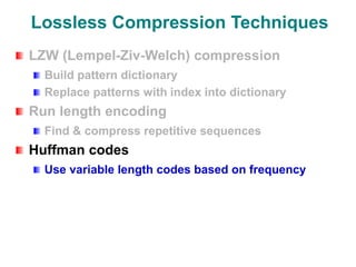
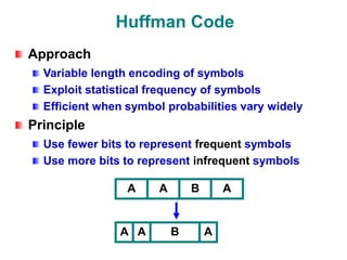
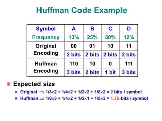
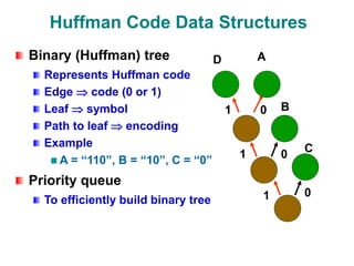
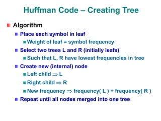
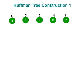
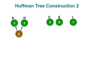
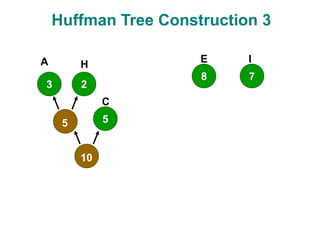
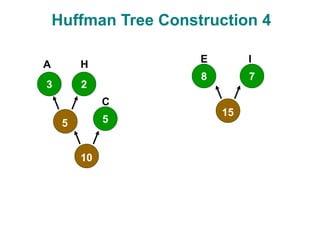
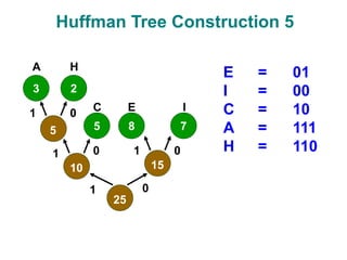
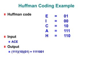
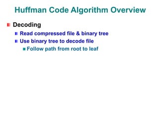
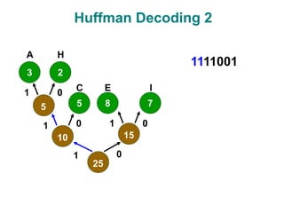
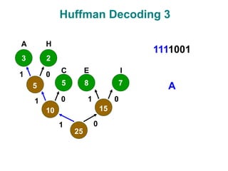
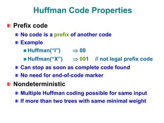
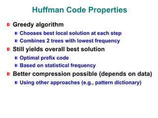
Compression & Huffman Codes
Compression
Definition
Reduce size of data
(number of bits needed to represent data)
Benefits
Reduce storage needed
Reduce transmission cost / latency / bandwidth
Sources of Compressibility
Redundancy
Recognize repeating patterns
Exploit using
Dictionary
Variable length encoding
Human perception
Less sensitive to some information
Can discard less important data
Types of Compression
Lossless
Preserves all information
Exploits redundancy in data
Applied to general data
Lossy
May lose some information
Exploits redundancy & human perception
Applied to audio, image, video
Effectiveness of Compression
Metrics
Bits per byte (8 bits)
2 bits / byte  ¼ original size
8 bits / byte  no compression
Percentage
75% compression  ¼ original size
Effectiveness of Compression
Depends on data
Random data  hard
Example: 1001110100  ?
Organized data  easy
Example: 1111111111  110
Corollary
No universally best compression algorithm
Effectiveness of Compression
Lossless Compression is not always possible
If compression is always possible (alternative view)
Compress file (reduce size by 1 bit)
Recompress output
Repeat (until we can store data with 0 bits)
Lossless Compression Techniques
LZW (Lempel-Ziv-Welch) compression
Build pattern dictionary
Replace patterns with index into dictionary
Run length encoding
Find & compress repetitive sequences
Huffman codes
Use variable length codes based on frequency
Huffman Code
Approach
Variable length encoding of symbols
Exploit statistical frequency of symbols
Efficient when symbol probabilities vary widely
Principle
Use fewer bits to represent frequent symbols
Use more bits to represent infrequent symbols
A A B A
A A
A B
Huffman Code Example
Expected size
Original  1/82 + 1/42 + 1/22 + 1/82 = 2 bits / symbol
Huffman  1/83 + 1/42 + 1/21 + 1/83 = 1.75 bits / symbol
Symbol A B C D
Frequency 13% 25% 50% 12%
Original
Encoding
00 01 10 11
2 bits 2 bits 2 bits 2 bits
Huffman
Encoding
110 10 0 111
3 bits 2 bits 1 bit 3 bits
Huffman Code Data Structures
Binary (Huffman) tree
Represents Huffman code
Edge  code (0 or 1)
Leaf  symbol
Path to leaf  encoding
Example
A = “110”, B = “10”, C = “0”
Priority queue
To efficiently build binary tree 1
1 0
0
D
C
B
A
0
1
Huffman Code Algorithm Overview
Encoding
Calculate frequency of symbols in file
Create binary tree representing “best” encoding
Use binary tree to encode compressed file
For each symbol, output path from root to leaf
Size of encoding = length of path
Save binary tree
Huffman Code – Creating Tree
Algorithm
Place each symbol in leaf
Weight of leaf = symbol frequency
Select two trees L and R (initially leafs)
Such that L, R have lowest frequencies in tree
Create new (internal) node
Left child  L
Right child  R
New frequency  frequency( L ) + frequency( R )
Repeat until all nodes merged into one tree
Huffman Tree Construction 1
3 5 8 2 7
A C E H I
Huffman Tree Construction 2
3 5 8
2 7
5
A C E
H I
Huffman Tree Construction 3
3
5
8
2
7
5
10
A
C
E
H
I
Huffman Tree Construction 4
3
5
8
2
7
5
10
15
A
C
E
H
I
Huffman Tree Construction 5
3
5 8
2
7
5
10 15
25
1
1
1
1
0
0
0
0
A
C E
H
I
E = 01
I = 00
C = 10
A = 111
H = 110
Huffman Coding Example
Huffman code
Input
ACE
Output
(111)(10)(01) = 1111001
E = 01
I = 00
C = 10
A = 111
H = 110
Huffman Code Algorithm Overview
Decoding
Read compressed file & binary tree
Use binary tree to decode file
Follow path from root to leaf
Huffman Decoding 1
3
5 8
2
7
5
10 15
25
1
1
1
1
0
0
0
0
A
C E
H
I
1111001
Huffman Decoding 2
3
5 8
2
7
5
10 15
25
1
1
1
1
0
0
0
0
A
C E
H
I
1111001
Huffman Decoding 3
3
5 8
2
7
5
10 15
25
1
1
1
1
0
0
0
0
A
C E
H
I
1111001
A
Huffman Decoding 4
3
5 8
2
7
5
10 15
25
1
1
1
1
0
0
0
0
A
C E
H
I
1111001
A
Huffman Decoding 5
3
5 8
2
7
5
10 15
25
1
1
1
1
0
0
0
0
A
C E
H
I
1111001
AC
Huffman Decoding 6
3
5 8
2
7
5
10 15
25
1
1
1
1
0
0
0
0
A
C E
H
I
1111001
AC
Huffman Decoding 7
3
5 8
2
7
5
10 15
25
1
1
1
1
0
0
0
0
A
C E
H
I
1111001
ACE
Huffman Code Properties
Prefix code
No code is a prefix of another code
Example
Huffman(“I”)  00
Huffman(“X”)  001 // not legal prefix code
Can stop as soon as complete code found
No need for end-of-code marker
Nondeterministic
Multiple Huffman coding possible for same input
If more than two trees with same minimal weight
Huffman Code Properties
Greedy algorithm
Chooses best local solution at each step
Combines 2 trees with lowest frequency
Still yields overall best solution
Optimal prefix code
Based on statistical frequency
Better compression possible (depends on data)
Using other approaches (e.g., pattern dictionary)

compression & huffman coder problem .ppt

  • 1.
  • 2.
    Compression Definition Reduce size ofdata (number of bits needed to represent data) Benefits Reduce storage needed Reduce transmission cost / latency / bandwidth
  • 3.
    Sources of Compressibility Redundancy Recognizerepeating patterns Exploit using Dictionary Variable length encoding Human perception Less sensitive to some information Can discard less important data
  • 4.
    Types of Compression Lossless Preservesall information Exploits redundancy in data Applied to general data Lossy May lose some information Exploits redundancy & human perception Applied to audio, image, video
  • 5.
    Effectiveness of Compression Metrics Bitsper byte (8 bits) 2 bits / byte  ¼ original size 8 bits / byte  no compression Percentage 75% compression  ¼ original size
  • 6.
    Effectiveness of Compression Dependson data Random data  hard Example: 1001110100  ? Organized data  easy Example: 1111111111  110 Corollary No universally best compression algorithm
  • 7.
    Effectiveness of Compression LosslessCompression is not always possible If compression is always possible (alternative view) Compress file (reduce size by 1 bit) Recompress output Repeat (until we can store data with 0 bits)
  • 8.
    Lossless Compression Techniques LZW(Lempel-Ziv-Welch) compression Build pattern dictionary Replace patterns with index into dictionary Run length encoding Find & compress repetitive sequences Huffman codes Use variable length codes based on frequency
  • 9.
    Huffman Code Approach Variable lengthencoding of symbols Exploit statistical frequency of symbols Efficient when symbol probabilities vary widely Principle Use fewer bits to represent frequent symbols Use more bits to represent infrequent symbols A A B A A A A B
  • 10.
    Huffman Code Example Expectedsize Original  1/82 + 1/42 + 1/22 + 1/82 = 2 bits / symbol Huffman  1/83 + 1/42 + 1/21 + 1/83 = 1.75 bits / symbol Symbol A B C D Frequency 13% 25% 50% 12% Original Encoding 00 01 10 11 2 bits 2 bits 2 bits 2 bits Huffman Encoding 110 10 0 111 3 bits 2 bits 1 bit 3 bits
  • 11.
    Huffman Code DataStructures Binary (Huffman) tree Represents Huffman code Edge  code (0 or 1) Leaf  symbol Path to leaf  encoding Example A = “110”, B = “10”, C = “0” Priority queue To efficiently build binary tree 1 1 0 0 D C B A 0 1
  • 12.
    Huffman Code AlgorithmOverview Encoding Calculate frequency of symbols in file Create binary tree representing “best” encoding Use binary tree to encode compressed file For each symbol, output path from root to leaf Size of encoding = length of path Save binary tree
  • 13.
    Huffman Code –Creating Tree Algorithm Place each symbol in leaf Weight of leaf = symbol frequency Select two trees L and R (initially leafs) Such that L, R have lowest frequencies in tree Create new (internal) node Left child  L Right child  R New frequency  frequency( L ) + frequency( R ) Repeat until all nodes merged into one tree
  • 14.
    Huffman Tree Construction1 3 5 8 2 7 A C E H I
  • 15.
    Huffman Tree Construction2 3 5 8 2 7 5 A C E H I
  • 16.
    Huffman Tree Construction3 3 5 8 2 7 5 10 A C E H I
  • 17.
    Huffman Tree Construction4 3 5 8 2 7 5 10 15 A C E H I
  • 18.
    Huffman Tree Construction5 3 5 8 2 7 5 10 15 25 1 1 1 1 0 0 0 0 A C E H I E = 01 I = 00 C = 10 A = 111 H = 110
  • 19.
    Huffman Coding Example Huffmancode Input ACE Output (111)(10)(01) = 1111001 E = 01 I = 00 C = 10 A = 111 H = 110
  • 20.
    Huffman Code AlgorithmOverview Decoding Read compressed file & binary tree Use binary tree to decode file Follow path from root to leaf
  • 21.
    Huffman Decoding 1 3 58 2 7 5 10 15 25 1 1 1 1 0 0 0 0 A C E H I 1111001
  • 22.
    Huffman Decoding 2 3 58 2 7 5 10 15 25 1 1 1 1 0 0 0 0 A C E H I 1111001
  • 23.
    Huffman Decoding 3 3 58 2 7 5 10 15 25 1 1 1 1 0 0 0 0 A C E H I 1111001 A
  • 24.
    Huffman Decoding 4 3 58 2 7 5 10 15 25 1 1 1 1 0 0 0 0 A C E H I 1111001 A
  • 25.
    Huffman Decoding 5 3 58 2 7 5 10 15 25 1 1 1 1 0 0 0 0 A C E H I 1111001 AC
  • 26.
    Huffman Decoding 6 3 58 2 7 5 10 15 25 1 1 1 1 0 0 0 0 A C E H I 1111001 AC
  • 27.
    Huffman Decoding 7 3 58 2 7 5 10 15 25 1 1 1 1 0 0 0 0 A C E H I 1111001 ACE
  • 28.
    Huffman Code Properties Prefixcode No code is a prefix of another code Example Huffman(“I”)  00 Huffman(“X”)  001 // not legal prefix code Can stop as soon as complete code found No need for end-of-code marker Nondeterministic Multiple Huffman coding possible for same input If more than two trees with same minimal weight
  • 29.
    Huffman Code Properties Greedyalgorithm Chooses best local solution at each step Combines 2 trees with lowest frequency Still yields overall best solution Optimal prefix code Based on statistical frequency Better compression possible (depends on data) Using other approaches (e.g., pattern dictionary)