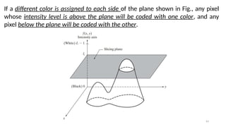
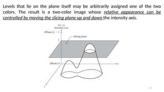
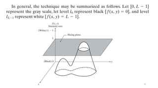
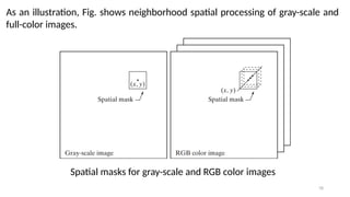
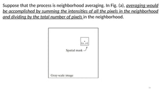
Download to read offline
![5
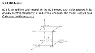
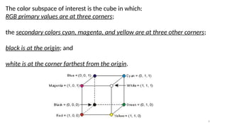
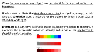
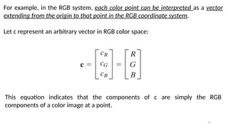
In this model, the gray scale (points of equal RGB values) extends from black to
white along the line joining these two points. For convenience, the assumption
is that all color values have been normalized so that the cube is the unit cube.
That is, all values of R, G, and B are assumed to be in the range [0, 1].](https://image.slidesharecdn.com/digitalimageprocessinglecture5-250817160959-0e227b3d/85/Color-Image-Processing-Digital-Image-Processing-Lecture-5-5-320.jpg)
![6
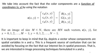
The number of bits used to represent each pixel in RGB space is called the pixel
depth.
Consider an RGB image in which each of the red, green, and blue images is an 8-
bit image. Under these conditions each RGB color pixel [that is, a triplet of
values (R, G, B)] is said to have a depth of 24 bits (3 image planes times the
number of bits per plane).
The term full-color image is used often to
denote a 24-bit RGB color image.
The total number of colors in a 24-bit
RGB image is](https://image.slidesharecdn.com/digitalimageprocessinglecture5-250817160959-0e227b3d/85/Color-Image-Processing-Digital-Image-Processing-Lecture-5-6-320.jpg)
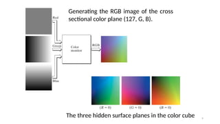
![8
For instance, a cross-sectional plane through the center of the cube and parallel
to the GB-plane is the plane (127, G, B) for
Here we used the actual pixel values rather than the mathematically convenient
normalized values in the range [0, 1] because the former values are the ones
actually used in a computer to generate colors.](https://image.slidesharecdn.com/digitalimageprocessinglecture5-250817160959-0e227b3d/85/Color-Image-Processing-Digital-Image-Processing-Lecture-5-8-320.jpg)
![13
Most devices that deposit colored pigments on paper, such as color printers and
copiers, require CMY data input or perform an RGB to CMY conversion
internally.
Cyan = White – Red
Magenta = White – Green
Yellow = White – Blue
This conversion is performed using the simple operation
Where, again, the assumption is that all color values have been normalized to
the range [0, 1].](https://image.slidesharecdn.com/digitalimageprocessinglecture5-250817160959-0e227b3d/85/Color-Image-Processing-Digital-Image-Processing-Lecture-5-13-320.jpg)
![20
Thus, if we wanted to determine the intensity component of any color point in
Fig, we would simply pass a plane perpendicular to the intensity axis and
containing the color point. The intersection of the plane with the intensity axis
would give us a point with intensity value in the range [0, 1].](https://image.slidesharecdn.com/digitalimageprocessinglecture5-250817160959-0e227b3d/85/Color-Image-Processing-Digital-Image-Processing-Lecture-5-20-320.jpg)
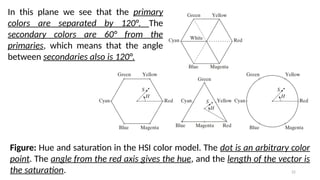
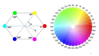
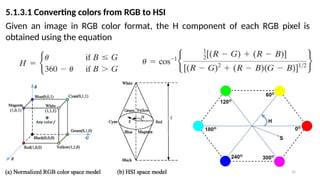
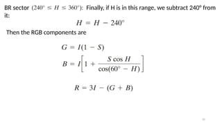
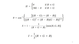
![26
The saturation component is given by
Finally, the intensity component is given by
It is assumed that the RGB values have been normalized to the range [0, 1] and
that angle is measured with respect to the red axis of the HSI space.
Hue can be normalized to the range [0, 1] by dividing by 360° all values
resulting from Eq.
The other two HSI components already are in this range if the given RGB
values are in the interval [0, 1].](https://image.slidesharecdn.com/digitalimageprocessinglecture5-250817160959-0e227b3d/85/Color-Image-Processing-Digital-Image-Processing-Lecture-5-26-320.jpg)
![27
Steps of Conversion
Normalize the RGB Values:
First, convert the RGB values to the [0, 1] range by dividing each component by
255. For example, consider a pixel with RGB values (100, 150, 200):](https://image.slidesharecdn.com/digitalimageprocessinglecture5-250817160959-0e227b3d/85/Color-Image-Processing-Digital-Image-Processing-Lecture-5-27-320.jpg)
![29
Calculate Hue (H):
Hue represents the color type and is calculated using:
Finally, normalize to the [0, 1] range by dividing by 360°.
𝐻](https://image.slidesharecdn.com/digitalimageprocessinglecture5-250817160959-0e227b3d/85/Color-Image-Processing-Digital-Image-Processing-Lecture-5-29-320.jpg)
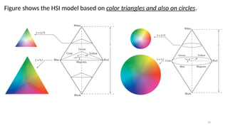
![32
5.1.3.2 Converting colors from HSI to RGB
Given values of HSI in the interval [0, 1], we now want to find the corresponding
RGB values in the same range.
The applicable equations depend on the
values of H.
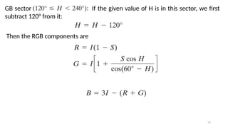
There are three sectors of interest,
corresponding to the 120° intervals in the
separation of primaries.](https://image.slidesharecdn.com/digitalimageprocessinglecture5-250817160959-0e227b3d/85/Color-Image-Processing-Digital-Image-Processing-Lecture-5-32-320.jpg)
![33
We begin by multiplying H by 360°, which returns the hue to its original range
of [0°, 360°].
RG sector : When H is in this sector, the RGB components are given
by the equations](https://image.slidesharecdn.com/digitalimageprocessinglecture5-250817160959-0e227b3d/85/Color-Image-Processing-Digital-Image-Processing-Lecture-5-33-320.jpg)
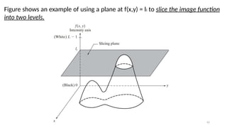
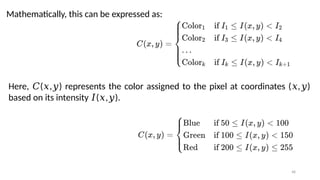
![47
Let ( , ) represent the intensity function of the image, where and are
𝐼 𝑥 𝑦 𝑥 𝑦
spatial coordinates, and ( , ) is the intensity at that point.
𝐼 𝑥 𝑦
Define Intensity Range:
Define a set of intensity intervals [𝐼1,𝐼2],[𝐼3,𝐼4],…,[𝐼𝑘,𝐼 +1
𝑘 ], where each interval
corresponds to a different color range.
Assign Color:
For each pixel with intensity value ( , ), assign a color based on which interval
𝐼 𝑥 𝑦
the intensity value falls into.](https://image.slidesharecdn.com/digitalimageprocessinglecture5-250817160959-0e227b3d/85/Color-Image-Processing-Digital-Image-Processing-Lecture-5-47-320.jpg)

This lecture introduces the fundamentals of color representation and processing in the digital domain. It covers color models (RGB, CMY, HSV, HSI), color transformations, enhancement techniques, and color image segmentation. Applications in computer vision, multimedia, remote sensing, and medical imaging are highlighted to show the importance of color in image analysis.