AAAAA

1. Computer Vision - A
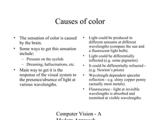
Causes of color
• The sensation of color is caused
by the brain.
• Some ways to get this sensation
include:
– Pressure on the eyelids
– Dreaming, hallucinations, etc.
• Main way to get it is the
response of the visual system to
the presence/absence of light at
various wavelengths.
• Light could be produced in
different amounts at different
wavelengths (compare the sun and
a fluorescent light bulb).
• Light could be differentially
reflected (e.g. some pigments).
• It could be differentially refracted -
(e.g. Newton’s prism)
• Wavelength dependent specular
reflection - e.g. shiny copper penny
(actually most metals).
• Flourescence - light at invisible
wavelengths is absorbed and
reemitted at visible wavelengths.

2. Computer Vision - A
Radiometry for colour
• All definitions are now “per unit wavelength”
• All units are now “per unit wavelength”
• All terms are now “spectral”
• Radiance becomes spectral radiance
– watts per square meter per steradian per unit wavelength
• Radiosity --- spectral radiosity

3. Computer Vision - A
Black body radiators
• Construct a hot body with near-zero albedo (black body)
– Easiest way to do this is to build a hollow metal object with a tiny
hole in it, and look at the hole.
• The spectral power distribution of light leaving this object
is a simple function of temperature
• This leads to the notion of color temperature --- the
temperature of a black body that would look the same
E λ( ) ∝
1
λ5
⎛
⎝
⎞
⎠
1
exp hc kλT( )−1
⎛
⎝
⎜
⎞
⎠
⎟

4. Computer Vision - A
Measurements of
relative spectral power
of sunlight, made by J.
Parkkinen and P.
Silfsten. Relative
spectral power is plotted
against wavelength in
nm. The visible range is
about 400nm to 700nm.
The color names on the
horizontal axis give the
color names used for
monochromatic light of
the corresponding
wavelength --- the
“colors of the rainbow”.
Mnemonic is “Richard
of York got blisters in
Venice”.
Violet Indigo Blue Green Yellow Orange Red

5. Computer Vision - A
Relative spectral power
of two standard
illuminant models ---
D65 models sunlight,and
illuminant A models
incandescent lamps.
Relative spectral power
is plotted against
wavelength in nm. The
visible range is about
400nm to 700nm. The
color names on the
horizontal axis give the
color names used for
monochromatic light of
the corresponding
wavelength --- the
“colors of the rainbow”.
Violet Indigo Blue Green Yellow Orange Red

6. Computer Vision - A
Measurements of
relative spectral power
of four different
artificial illuminants,
made by H.Sugiura.
Relative spectral power
is plotted against
wavelength in nm. The
visible range is about
400nm to 700nm.

7. Computer Vision - A
Spectral albedoes for
several different leaves,
with color names
attached. Notice that
different colours
typically have different
spectral albedo, but that
different spectral
albedoes may result in
the same perceived
color (compare the two
whites). Spectral
albedoes are typically
quite smooth functions.
Measurements by
E.Koivisto.

8. Computer Vision - A
The appearance of colors
• Color appearance is strongly
affected by (at least):
– other nearby colors,
– adaptation to previous views
– “state of mind”
• We show several demonstrations in
what follows.
• Film color mode:
View a colored surface
through a hole in a sheet, so that
the colour looks like a film in
space; controls for nearby colors,
and state of mind.
• Other modes:
– Surface colour
– Volume colour
– Mirror colour
– Illuminant colour

9. Computer Vision - A
The appearance of colors
• Hering, Helmholtz: Color appearance is
strongly affected by other nearby
colors, by adaptation to previous views,
and by “state of mind”
• Film color mode: View a
colored surface through a hole in a
sheet, so that the colour looks like a
film in space; controls for nearby
colors, and state of mind.
– Other modes:
• Surface colour
• Volume colour
• Mirror colour
• Illuminant colour
• By experience, it is possible to
match almost all colors, viewed in
film mode using only three primary
sources - the principle of
trichromacy.
– Other modes may have more
dimensions
• Glossy-matte
• Rough-smooth
• Most of what follows discusses
film mode.

10. Computer Vision - A

11. Computer Vision - A

12. Computer Vision - A

13. Computer Vision - A
Why specify color numerically?
• Accurate color reproduction is
commercially valuable
– Many products are identified by
color (“golden” arches;
• Few color names are widely
recognized by English speakers -
– About 10; other languages have
fewer/more, but not many more.
– It’s common to disagree on
appropriate color names.
• Color reproduction problems
increased by prevalence of digital
imaging - eg. digital libraries of art.
– How do we ensure that everyone
sees the same color?

14. Computer Vision - A
Color matching experiments - I
• Show a split field to subjects; one side shows the light
whose color one wants to measure, the other a weighted
mixture of primaries (fixed lights).
• Each light is seen in film color mode.

15. Computer Vision - A
Color matching experiments - II
• Many colors can be represented as a mixture of A, B, C
• write
M=a A + b B + c C
where the = sign should be read as “matches”
• This is additive matching.
• Gives a color description system - two people who agree
on A, B, C need only supply (a, b, c) to describe a color.

16. Computer Vision - A
Subtractive matching
• Some colors can’t be matched like this:
instead, must write
M+a A = b B+c C
• This is subtractive matching.
• Interpret this as (-a, b, c)
• Problem for building monitors: Choose R, G, B such
that positive linear combinations match a large set of
colors

17. Computer Vision - A
The principle of trichromacy
• Experimental facts:
– Three primaries will work for most people if we allow subtractive
matching
• Exceptional people can match with two or only one primary.
• This could be caused by a variety of deficiencies.
– Most people make the same matches.
• There are some anomalous trichromats, who use three
primaries but make different combinations to match.

18. Computer Vision - A
Grassman’s Laws
• For colour matches made in film colour mode:
– symmetry: U=V <=>V=U
– transitivity: U=V and V=W => U=W
– proportionality: U=V <=> tU=tV
– additivity: if any two (or more) of the statements
U=V,
W=X,
(U+W)=(V+X) are true, then so is the third
• These statements are as true as any biological law. They
mean that color matching in film color mode is linear.

19. Computer Vision - A
Linear color spaces
• A choice of primaries yields a
linear color space --- the
coordinates of a color are given
by the weights of the primaries
used to match it.
• Choice of primaries is
equivalent to choice of color
space.
• RGB: primaries are
monochromatic energies are
645.2nm, 526.3nm, 444.4nm.
• CIE XYZ: Primaries are
imaginary, but have other
convenient properties. Color
coordinates are (X,Y,Z), where
X is the amount of the X
primary, etc.
– Usually draw x, y, where
x=X/(X+Y+Z) y=Y/
(X+Y+Z)

20. Computer Vision - A
Color matching functions
• Choose primaries, say A, B, C
• Given energy function,
what amounts of primaries will
match it?
• For each wavelength, determine
how much of A, of B, and of C
is needed to match light of that
wavelength alone.
• These are colormatching
functions
a(λ)
β(λ)
χ(λ)
E(λ) Then our match is:
a(λ)E(λ)dλ∫{ }A +
b(λ)E(λ)dλ∫{ }B +
c(λ)E(λ)dλ∫{ }C

21. Computer Vision - A
RGB: primaries are
monochromatic, energies are
645.2nm, 526.3nm, 444.4nm.
Color matching functions have
negative parts -> some colors
can be matched only
subtractively.

22. Computer Vision - A
CIE XYZ: Color
matching functions are
positive everywhere, but
primaries are imaginary.
Usually draw x, y, where
x=X/(X+Y+Z)
y=Y/(X+Y+Z)

23. Computer Vision - A
A qualitative rendering of
the CIE (x,y) space. The
blobby region represents
visible colors. There are
sets of (x, y) coordinates
that don’t represent real
colors, because the
primaries are not real lights
(so that the color matching
functions could be positive
everywhere).

24. Computer Vision - A
A plot of the CIE (x,y)
space. We show the
spectral locus (the colors
of monochromatic
lights) and the black-
body locus (the colors of
heated black-bodies). I
have also plotted the
range of typical
incandescent lighting.

25. Computer Vision - A
Non-linear colour spaces
• HSV: Hue, Saturation, Value are non-linear functions of
XYZ.
– because hue relations are naturally expressed in a circle
• Uniform: equal (small!) steps give the same perceived
color changes.
• Munsell: describes surfaces, rather than lights - less
relevant for graphics. Surfaces must be viewed under
fixed comparison light

26. Computer Vision - A
HSV hexcone

27. Computer Vision - A
Uniform color spaces
• McAdam ellipses (next slide) demonstrate that differences
in x,y are a poor guide to differences in color
• Construct color spaces so that differences in coordinates
are a good guide to differences in color.

28. Computer Vision - A
Variations in color matches on a CIE x, y space. At the center of the ellipse is the color of a
test light; the size of the ellipse represents the scatter of lights that the human observers
tested would match to the test color; the boundary shows where the just noticeable difference
is. The ellipses on the left have been magnified 10x for clarity; on the right they are plotted
to scale. The ellipses are known as MacAdam ellipses after their inventor. The ellipses at the
top are larger than those at the bottom of the figure, and that they rotate as they move up.
This means that the magnitude of the difference in x, y coordinates is a poor guide to the
difference in color.

29. Computer Vision - A
CIE u’v’ which is a
projective transform
of x, y. We transform
x,y so that ellipses are
most like one another.
Figure shows the
transformed ellipses.

30. Computer Vision - A
Color receptors and color deficiency
• Trichromacy is justified - in
color normal people, there are
three types of color receptor,
called cones, which vary in
their sensitivity to light at
different wavelengths (shown
by molecular biologists).
• Deficiency can be caused by
CNS, by optical problems in the
eye, or by absent receptor types
– Usually a result of absent
genes.
• Some people have fewer than
three types of receptor; most
common deficiency is red-green
color blindness in men.
• Color deficiency is less
common in women; red and
green receptor genes are carried
on the X chromosome, and
these are the ones that typically
go wrong. Women need two
bad X chromosomes to have a
deficiency, and this is less
likely.

31. Computer Vision - A
Color receptors
• Principle of univariance:
cones give the same kind of
response, in different amounts,
to different wavelengths. The
output of the cone is obtained
by summing over wavelengths.
Responses are measured in a
variety of ways (comparing
behaviour of color normal and
color deficient subjects).
• All experimental evidence
suggests that the response of
the k’th type of cone can be
written as
where is the sensitivity
of the receptor and spectral
energy density of the incoming
light.
ρ∫ k
(λ)E(λ)dλ
ρk (λ)

32. Computer Vision - A
Color receptors
• Plot shows relative sensitivity
as a function of wavelength, for
the three cones. The S (for
short) cone responds most
strongly at short wavelengths;
the M (for medium) at medium
wavelengths and the L (for
long) at long wavelengths.
• These are occasionally called B,
G and R cones respectively, but
that’s misleading - you don’t
see red because your R cone is
activated.

33. Computer Vision - A
Adaptation phenomena
• The response of your color
system depends both on spatial
contrast and what it has seen
before (adaptation)
• This seems to be a result of
coding constraints --- receptors
appear to have an operating
point that varies slowly over
time, and to signal some sort of
offset. One form of adaptation
involves changing this
operating point.
• Common example: walk inside
from a bright day; everything
looks dark for a bit, then takes
its conventional brightness.

34. Computer Vision - A

35. Computer Vision - A

36. Computer Vision - A

37. Computer Vision - A

38. Computer Vision - A

39. Computer Vision - A

40. Computer Vision - A

41. Computer Vision - A

42. Computer Vision - A
Viewing coloured objects
• Assume diffuse+specular model
• Specular
– specularities on dielectric
objects take the colour of the
light
– specularities on metals can be
coloured
• Diffuse
– colour of reflected light
depends on both illuminant
and surface
– people are surprisingly good at
disentangling these effects in
practice (colour constancy)
– this is probably where some of
the spatial phenomena in
colour perception come from

43. Computer Vision - A
When one views a colored
surface, the spectral
radiance of the light
reaching the eye depends
on both the spectral
radiance of the illuminant,
and on the spectral albedo
of the surface. We’re
assuming that camera
receptors are linear, like
the receptors in the eye.
This is usually the case.

44. Computer Vision - A
Subtractive mixing of inks
• Inks subtract light from white,
whereas phosphors glow.
• Linearity depends on pigment
properties
– inks, paints, often hugely non-
linear.
• Inks: Cyan=White-Red,
Magenta=White-Green,
Yellow=White-Blue.
• For a good choice of inks, and
good registration, matching is
linear and easy
• eg. C+M+Y=White-
White=Black
C+M=White-Yellow=Blue
• Usually require CMY and
Black, because colored inks are
more expensive, and
registration is hard
• For good choice of inks, there
is a linear transform between
XYZ and CMY

45. Computer Vision - A
Finding Specularities
• Assume we are dealing with dielectrics
– specularly reflected light is the same color as the source
• Reflected light has two components
– diffuse
– specular
– and we see a weighted sum of these two
• Specularities produce a characteristic dogleg in the
histogram of receptor responses
– in a patch of diffuse surface, we see a color multiplied by different
scaling constants (surface orientation)
– in the specular patch, a new color is added; a “dog-leg” results

46. Computer Vision - A
R
G
B
Illuminant color
Dif fuse component
T
S

47. Computer Vision - A
R
G
B
R
G
B
Dif fuse
region
Boundary of
specularity

48. Computer Vision - A
Color constancy
• Assume we’ve identified and removed specularities
• The spectral radiance at the camera depends on two things
– surface albedo
– illuminant spectral radiance
– the effect is much more pronounced than most people think (see following
slides)
• We would like an illuminant invariant description of the surface
– e.g. some measurements of surface albedo
– need a model of the interactions
• Multiple types of report
– The colour of paint I would use is
– The colour of the surface is
– The colour of the light is

49. Computer Vision - A
Notice how the
color of light at
the camera varies
with the illuminant
color; here we have
a uniform reflectance
illuminated by five
different lights, and
the result plotted on
CIE x,y

50. Computer Vision - A
Notice how the
color of light at
the camera varies
with the illuminant
color; here we have
the blue flower
illuminated by five
different lights, and
the result plotted on
CIE x,y. Notice how it
looks significantly more
saturated under some
lights.

51. Computer Vision - A
Notice how the
color of light at
the camera varies
with the illuminant
color; here we have
a green leaf
illuminated by five
different lights, and
the result plotted on
CIE x,y

52. Computer Vision - A

53. Computer Vision - A

54. Computer Vision - A

55. Computer Vision - A
Land’s Demonstration

56. Computer Vision - A
Lightness Constancy
• Lightness constancy
– how light is the surface, independent of the brightness of the illuminant
– issues
• spatial variation in illumination
• absolute standard
– Human lightness constancy is very good
• Assume
– frontal 1D “Surface”
– slowly varying illumination
– quickly varying surface reflectance

57. Computer Vision - A

58. Computer Vision - A

59. Computer Vision - A
Lightness Constancy in 2D
• Differentiation, thresholding
are easy
– integration isn’t
– problem - gradient field may
no longer be a gradient field
• One solution
– Choose the function whose
gradient is “most like”
thresholded gradient
• This yields a minimization
problem
• How do we choose the constant
of integration?
– average lightness is grey
– lightest object is white
– ?

60. Computer Vision - A
Simplest colour constancy
• Adjust three receptor channels independently
– Von Kries
– Where does the constant come from?
• White patch
• Averages
• Some other known reference (faces, nose)

61. Computer Vision - A
Colour Constancy - I
• We need a model of interaction
between illumination and
surface colour
– finite dimensional linear model
seems OK
• Finite Dimensional Linear
Model (or FDLM)
– surface spectral albedo is a
weighted sum of basis
functions
– illuminant spectral exitance is
a weighted sum of basis
functions
– This gives a quite simple form
to interaction between the two

62. Computer Vision - A
Finite Dimensional Linear Models
E λ( ) = εiψi λ( )
i=1
m
∑
ρ λ( ) = rjϕj λ( )
j=1
n
∑
pk = σ k λ( ) εiψi λ( )
i=1
m
∑
⎛
⎝
⎜
⎞
⎠
⎟ rjϕj λ( )
j=1
n
∑
⎛
⎝
⎜⎜
⎞
⎠
⎟⎟dλ∫
= εirj σk λ( )ψi λ( )ϕj λ( )dλ∫
i=1,j=1
m,n
∑
= εirj gijk
i=1,j=1
m,n
∑

63. Computer Vision - A
General strategies
• Determine what image would
look like under white light
• Assume
– that we are dealing with flat
frontal surfaces
– We’ve identified and removed
specularities
– no variation in illumination
• We need some form of
reference
– brightest patch is white
– spatial average is known
– gamut is known
– specularities

64. Computer Vision - A
Obtaining the illuminant from
specularities
• Assume that a specularity has
been identified, and material is
dielectric.
• Then in the specularity, we
have
• Assuming
– we know the sensitivities and
the illuminant basis functions
– there are no more illuminant
basis functions than receptors
• This linear system yields the
illuminant coefficients.pk = σk λ( )E λ( )∫ dλ
= εi σk λ( )ψi λ( )∫ dλ
i=1
m
∑

65. Computer Vision - A
Obtaining the illuminant from average
color assumptions
• Assume the spatial average
reflectance is known
• We can measure the spatial
average of the receptor
response to get
• Assuming
– g_ijk are known
– average reflectance is known
– there are not more receptor
types than illuminant basis
functions
• We can recover the illuminant
coefficients from this linear
system
ρ λ( ) = r jϕj λ( )
j=1
n
∑
pk = εi r j gijk
i=1,j=1
m,n
∑

66. Computer Vision - A
Computing surface properties
• Two strategies
– compute reflectance
coefficients
– compute appearance under
white light.
• These are essentially
equivalent.
• Once illuminant coefficients are
known, to get reflectance
coefficients we solve the linear
system
• to get appearance under white
light, plug in reflectance
coefficients and compute
pk = εirj gijk
i=1,j=1
m,n
∑
pk = εi
white
rj gijk
i=1,j=1
m,n
∑