human resource and management

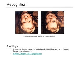
1. Recognition
Readings
• C. Bishop, “Neural Networks for Pattern Recognition”, Oxford University
Press, 1998, Chapter 1.
• Szeliski, Chapter 14.2.1 (eigenfaces)
The “Margaret Thatcher Illusion”, by Peter Thompson

2. Recognition
The “Margaret Thatcher Illusion”, by Peter Thompson

3. What do we mean by “recognition”?
Next 15 slides adapted from
Li, Fergus, & Torralba’s
excellent short course on
category and object recognition

4. Verification: is that a lamp?

5. Detection: are there people?

6. Identification: is that Potala Palace?

7. Object categorization
mountain
building
tree
banner
vendor
people
street lamp

8. Scene and context categorization
• outdoor
• city
• …

9. Applications: Computational photography

10. Applications: Assisted driving
meters
meters
Ped
Ped
Car
Lane detection
Pedestrian and car detection
• Collision warning systems
with adaptive cruise control,
• Lane departure warning
systems,
• Rear object detection
systems,

11. Applications: image search

12. Challenges: viewpoint variation
Michelangelo 1475-1564

13. slide credit: S. Ullman
Challenges: illumination variation

14. Magritte, 1957
Challenges: occlusion

15. Challenges: scale

16. Challenges: deformation
Xu, Beihong 1943

17. Klimt, 1913
Challenges: background clutter

18. Challenges: intra-class variation

19. Face detection
How to tell if a face is present?

20. One simple method: skin detection
Skin pixels have a distinctive range of colors
• Corresponds to region(s) in RGB color space
– for visualization, only R and G components are shown above
skin
Skin classifier
• A pixel X = (R,G,B) is skin if it is in the skin region
• But how to find this region?

21. Skin detection
Learn the skin region from examples
• Manually label pixels in one or more “training images” as skin or not skin
• Plot the training data in RGB space
– skin pixels shown in orange, non-skin pixels shown in blue
– some skin pixels may be outside the region, non-skin pixels inside. Why?
Skin classifier
• Given X = (R,G,B): how to determine if it is skin or not?

22. Skin classification techniques
Skin classifier: Given X = (R,G,B): how to determine if it is skin or not?
• Nearest neighbor
– find labeled pixel closest to X
• Find plane/curve that separates the two classes
– popular approach: Support Vector Machines (SVM)
• Data modeling
– fit a model (curve, surface, or volume) to each class
– probabilistic version: fit a probability density/distribution model to each class

23. Probability
Basic probability
• X is a random variable
• P(X) is the probability that X achieves a certain value
•
• or
• Conditional probability: P(X | Y)
– probability of X given that we already know Y
continuous X discrete X
called a PDF
-probability distribution/density function
-a 2D PDF is a surface, 3D PDF is a volume

24. Probabilistic skin classification
Now we can model uncertainty
• Each pixel has a probability of being skin or not skin
–
Skin classifier
• Given X = (R,G,B): how to determine if it is skin or not?
• Choose interpretation of highest probability
– set X to be a skin pixel if and only if
Where do we get and ?

25. Learning conditional PDF’s
We can calculate P(R | skin) from a set of training images
• It is simply a histogram over the pixels in the training images
– each bin Ri contains the proportion of skin pixels with color Ri
This doesn’t work as well in higher-dimensional spaces. Why not?
Approach: fit parametric PDF functions
• common choice is rotated Gaussian
– center
– covariance
» orientation, size defined by eigenvecs, eigenvals

26. Learning conditional PDF’s
We can calculate P(R | skin) from a set of training images
• It is simply a histogram over the pixels in the training images
– each bin Ri contains the proportion of skin pixels with color Ri
But this isn’t quite what we want
• Why not? How to determine if a pixel is skin?
• We want P(skin | R) not P(R | skin)
• How can we get it?

27. Bayes rule
In terms of our problem:
what we measure
(likelihood)
domain knowledge
(prior)
what we want
(posterior)
normalization term
What could we use for the prior P(skin)?
• Could use domain knowledge
– P(skin) may be larger if we know the image contains a person
– for a portrait, P(skin) may be higher for pixels in the center
• Could learn the prior from the training set. How?
– P(skin) may be proportion of skin pixels in training set

28. Bayesian estimation
Bayesian estimation
• Goal is to choose the label (skin or ~skin) that maximizes the posterior
– this is called Maximum A Posteriori (MAP) estimation
likelihood posterior (unnormalized)
= minimize probability of misclassification

29. Bayesian estimation
Bayesian estimation
• Goal is to choose the label (skin or ~skin) that maximizes the posterior
– this is called Maximum A Posteriori (MAP) estimation
likelihood posterior (unnormalized)
0.5• Suppose the prior is uniform: P(skin) = P(~skin) =
= minimize probability of misclassification
– in this case ,
– maximizing the posterior is equivalent to maximizing the likelihood
» if and only if
– this is called Maximum Likelihood (ML) estimation

30. Skin detection results

31. This same procedure applies in more general circumstances
• More than two classes
• More than one dimension
General classification
H. Schneiderman and T.Kanade
Example: face detection
• Here, X is an image region
– dimension = # pixels
– each face can be thought
of as a point in a high
dimensional space
H. Schneiderman, T. Kanade. "A Statistical Method for 3D Object
Detection Applied to Faces and Cars". IEEE Conference on
Computer Vision and Pattern Recognition (CVPR 2000)
http://www-2.cs.cmu.edu/afs/cs.cmu.edu/user/hws/www/CVPR00.pdf

32. Linear subspaces
Classification can be expensive
• Big search prob (e.g., nearest neighbors) or store large PDF’s
Suppose the data points are arranged as above
• Idea—fit a line, classifier measures distance to line
convert x into v1, v2 coordinates
What does the v2 coordinate measure?
What does the v1 coordinate measure?
- distance to line
- use it for classification—near 0 for orange pts
- position along line
- use it to specify which orange point it is

33. Dimensionality reduction
Dimensionality reduction
• We can represent the orange points with only their v1 coordinates
– since v2 coordinates are all essentially 0
• This makes it much cheaper to store and compare points
• A bigger deal for higher dimensional problems

34. Linear subspaces
Consider the variation along direction v
among all of the orange points:
What unit vector v minimizes var?
What unit vector v maximizes var?
Solution: v1 is eigenvector of A with largest eigenvalue
v2 is eigenvector of A with smallest eigenvalue

35. Principal component analysis (PCA)
Suppose each data point is N-dimensional
• Same procedure applies:
• The eigenvectors of A define a new coordinate system
– eigenvector with largest eigenvalue captures the most variation among
training vectors x
– eigenvector with smallest eigenvalue has least variation
• We can compress the data by only using the top few eigenvectors
– corresponds to choosing a “linear subspace”
» represent points on a line, plane, or “hyper-plane”
– these eigenvectors are known as the principal components

36. The space of faces
An image is a point in a high dimensional space
• An N x M image is a point in RNM
• We can define vectors in this space as we did in the 2D case
+=

37. Dimensionality reduction
The set of faces is a “subspace” of the set of images
• Suppose it is K dimensional
• We can find the best subspace using PCA
• This is like fitting a “hyper-plane” to the set of faces
– spanned by vectors v1, v2, ..., vK
– any face

38. Eigenfaces
PCA extracts the eigenvectors of A
• Gives a set of vectors v1, v2, v3, ...
• Each one of these vectors is a direction in face space
– what do these look like?

39. Projecting onto the eigenfaces
The eigenfaces v1, ..., vK span the space of faces
• A face is converted to eigenface coordinates by

40. Recognition with eigenfaces
Algorithm
1. Process the image database (set of images with labels)
• Run PCA—compute eigenfaces
• Calculate the K coefficients for each image
1. Given a new image (to be recognized) x, calculate K coefficients
2. Detect if x is a face
1. If it is a face, who is it?
• Find closest labeled face in database
• nearest-neighbor in K-dimensional space

41. Choosing the dimension K
K NMi =
eigenvalues
How many eigenfaces to use?
Look at the decay of the eigenvalues
• the eigenvalue tells you the amount of variance “in the
direction” of that eigenface
• ignore eigenfaces with low variance

42. Object recognition
This is just the tip of the iceberg
• Better features:
– edges (e.g., SIFT)
– motion
– depth/3D info
– ...
• Better classifiers:
– e.g., support vector machines (SVN)
• Speed (e.g., real-time face detection)
• Scale
– e.g., Internet image search
Recognition is a very active research area right now