Downloaded 22 times
![H. Scott Fogler
Chapter 3 1/24/06
1
CD/CollisionTheory/ProfRef.doc
Professional Reference Shelf
A. Collision Theory
Overview – Collision Theory
In Chapter 3, we presented a number of rate laws that depended on both
concentration and temperature. For the elementary reaction
A + B → C + D
the elementary rate law is
!
"rA = kCACB = Ae"E RT
CACB
We want to provide at least a qualitative understanding of why the rate law takes this
form. We will first develop the collision rate, using collision theory for hard spheres of
cross section Sr,
!
"#AB
2
. When all collisions occur with the same relative velocity, UR, the
number of collisions between A and B molecules,
!
˜ZAB, is
!
˜ZAB =SrUR
˜CA
˜CB [collisions/s/molecule]
Next, we will consider a distribution of relative velocities and only consider those
collisions that have an energy of EA or greater in order to react to show
!
"rA = Ae"EA RT
CACB
where
!
A = "#AB
2 8kBT
"µAB
$
%
&
'
(
)
1 2
NAvo
with σAB = collision radius, kB = Boltzmann’s constant, µAB = reduced mass,
T = temperature, and NAvo = Avogadro’s number. To obtain an estimate of EA, we use
the Polyani Equation
!
EA = EA
o
+ "P#HRx
Where ΔHRx is the heat of reaction and
!
EA
o
and γP are the Polyani Parameters. With
these equations for A and EA we can make a first approximation to the rate law
parameters without going to the lab.](https://image.slidesharecdn.com/collisiontheory-160829145444/75/Collision-theory-1-2048.jpg)
![4
CD/CollisionTheory/ProfRef.doc
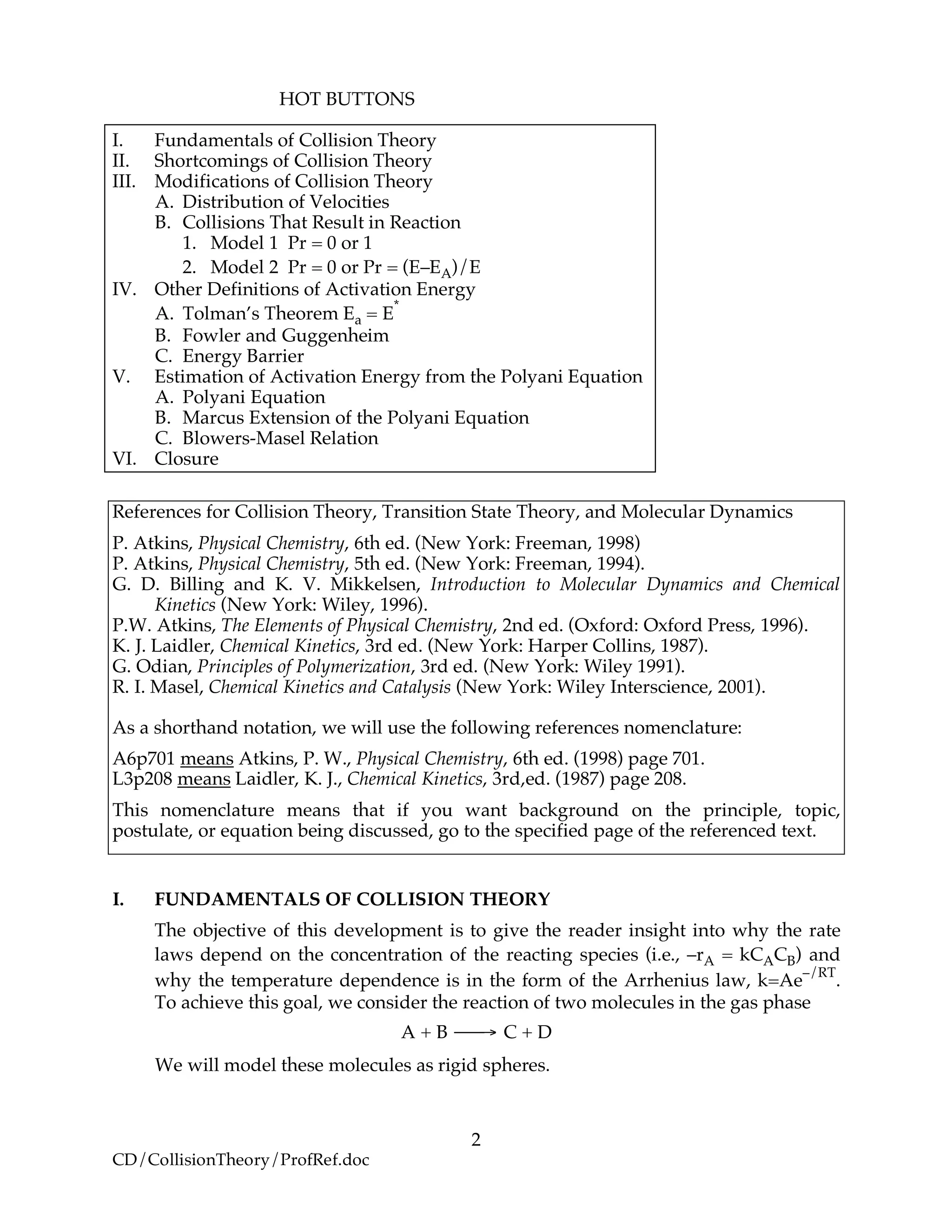
mA = mass of a molecule of species A (gm)
mB = mass of a molecule of species B (gm)
µAB = reduced mass =
mAmB
mA + mB
(g), [Let µ ≡ µAB]
MA = Molecular weight of A (Daltons)
NAvo = Avogadro’s number 6.022 molecules/mol
R = Ideal gas constant 8.314 J/mol•K = 8.314 kg • m
2
/s
2
/mol/K
We note that R = NAvo kB and MA = NAvo • mA, therefore we can write the ratio
(kB/µAB) as
!
kB
µAB
=
R
MAMB
MA +MB
"
#
$
$
$
$
%
&
'
'
'
'
(R3.A-2)
An order of magnitude of the relative velocity at 300 K is UR ! 3000 km hr,
i.e., ten times the speed of an Indianapolis 500 Formula 1 car. The collision
diameter and velocities at 0°C are given in Table R3.A-1.
Table R3.A-1 Molecular Diameters†
Molecule
Average Velocity,
(meters/second) Molecular Diameter (Å)
H2 1687 2.74
CO 453 3.12
Xe 209 4.85
He 1200 2.2
N2 450 3.5
O2 420 3.1
H2O 560 3.7
C2H6 437 5.3
C6H6 270 3.5
CH4 593 4.1
NH3 518 4.4
H2S 412 4.7
CO2 361 4.6
N2O 361 4.7
NO 437 3.7
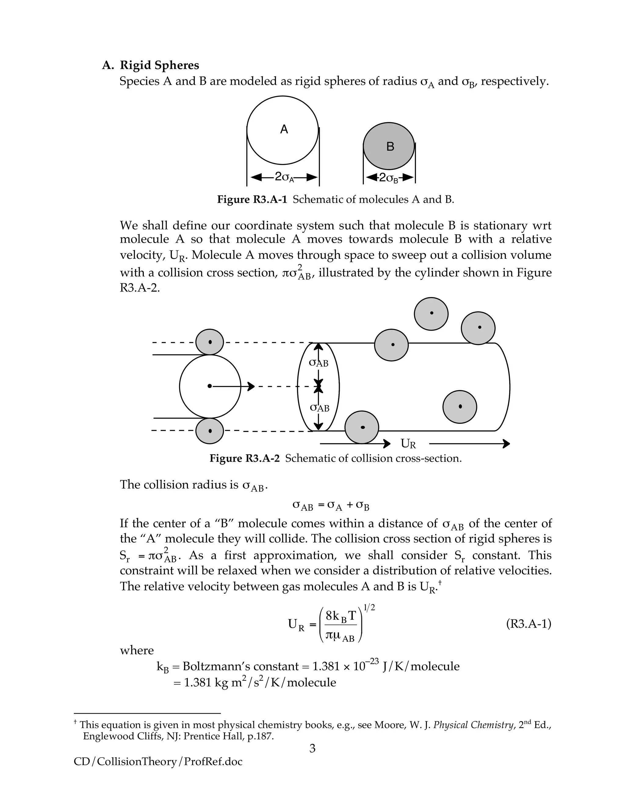
Consider a molecule A moving in space. In a time Δt, the volume ΔV swept out
by a molecule of A is
†
Courtesy of J. F. O’Hanlon, A User’s Guide to Vacuum Technology (New York: Wiley, 1980).](https://image.slidesharecdn.com/collisiontheory-160829145444/75/Collision-theory-4-2048.jpg)
![5
CD/CollisionTheory/ProfRef.doc
!V = UR!t( )
!l674 84
"#AB
2 !V
A
Figure R3.A-3 Volume swept out by molecule A in time Δt.
The bends in the volume represent that even though molecule A may change
directions upon collision the volume sweep out is the same. The number of
collisions that will take place will be equal to the number of B molecules,
ΔV ˜CB , that are in the volume swept out by the A molecule:
˜CB!V = No. of B molecules in !V[ ]
where ˜CB is in
!
molecules dm3
[ ] rather than [moles/dm
3
]
In a time Δt, the number of collisions of this one A molecule with many B
molecules is
!
UR
˜CB"#AB
2
$t. The number of collisions of this one A molecule
with all the B molecules per unit time is
˜Z1A• B = !"AB
2 ˜CBUR (R3.A-3)
However, we have many A molecules present at a concentration,
!
˜CA,
(molecule/dm
3
). Adding up the collisions of all the A molecules per unit
volume, ˜CA , then the number of collisions
!
˜ZAB of all the A molecules with all
B molecules per time per unit volume is
!
˜ZAB = "#AB
2
Sr
678
UR
˜CA
˜CB =SrUR
˜CA
˜CB (R3.A-4)
Where Sr is the collision cross section (Å)
2
. Substituting for Sr and UR
!
˜ZAB = "#AB
2 8kBT
"µ
$
%
&
'
(
)
1 2
˜CA
˜CB [molecules/time/volume] (R3.A-5)
If we assume all collisions result in reactions, then
!
"˜rA = ˜ZAB = #$AB
2 8kBT
#µ
%
&
'
(
)
*
1 2
˜CA
˜CB [molecules/time/volume] (R3.A-6)
Multiplying and dividing by Avogadrós number, NAvo, we can put our
equation for the rate of reaction in terms of the number of moles/time/vol.
!
"˜rA
NAvo
#
$
%
&
'
(
"rA
123
NAvo = )*AB
2 8kBT
)µ
#
$
%
&
'
(
1 2
˜CA
NAvo
CA
123
˜CB
NAvo
CB
123
NAvo
2
(R3.A-7)](https://image.slidesharecdn.com/collisiontheory-160829145444/75/Collision-theory-5-2048.jpg)
![6
CD/CollisionTheory/ProfRef.doc
!
"rA = #$AB
2 8#kBT
µ#
%
&
'
(
)
*
1 2
NAvo
A
1 24444 34444
CACB [moles/time/volume] (R3.A-8)
where A is the frequency factor
!
A = "AB
2 8#kBT
µAB
$
%
&
'
(
)
1 2
NAvo (R3.A-9)
!
"rA = ACACB (R3.A-10)
Example Calculate the frequency factor A for the reaction
!
H +O2 " OH +O
at 273K.
Additional information:
Using the values in Table R3.A-1
Collision Radii
Hydrogen H σH=2.74 Å/4 = 0.68Å = 0.68 x 10⁻¹⁰
m
Oxygen O2
!
"O2
=
3.1
2
Å 1.55Å = 1.5 x 10⁻¹⁰
m
!
R = 8.31J mol K = 8.314 kg m2
s2
K mol
Solution
!
A =SrURNAvo (R3.A-E-1)
!
A = "#AB
2
URNAvo = "#AB
2 8kBT
"µ
$
%
&
'
(
)
1 2
NAvo (R3.A-9)
The relative velocity is
!
UR =
8kBT
"µ
#
$
%
&
'
(
1 2
(R3.A-1)
Calculate the ratio kB/µAB (Let µ ≡ µAB)
!
kB
µ
=
R
MAMB
MA +MB
=
8.314 kg" m2
s2
K mol
1g mol( ) 32g mol( )
1g mol+ 32g mol
#
$
%
&
'
(
=
8.314kg•m2
s2
K mol
0.97 g mol)
1kg
1000g](https://image.slidesharecdn.com/collisiontheory-160829145444/75/Collision-theory-6-2048.jpg)
![7
CD/CollisionTheory/ProfRef.doc
!
kB
µ
= 8571m2
s2
K
Calculate the relative velocity
!
UR =
8( ) 273K( ) 8571( )m2
s2
K
3.14
"
#
$
$
%
&
'
'
1 2
= 2441m s = 2.44 (1013
Å s (R3.A-E-2)
!
Sr = "#AB
2
= " #A +#B[ ]
2
= " 0.68 $10%10
m +1.55 $10%10
m[ ]
2
=15.6 $10%20
m2
molecule
Calculate the frequency factor A
!
A =
15.6 "10#20
m2
molecule
2441m s[ ] 6.02 "1023
molecule mol[ ] (R3.A-E-3)
!
A = 2.29 "108 m3
mol#s
= 2.29 "1011 dm3
mol#s
(R3.A-E-4)
!
A = 2.29 "106 m3
mol#s
"
1mol
6.02 "1023
molecule
1010
Å
m
$
%
&
'
(
)
3
!
A = 3.81"1014
Å( )
3
molecule s (R3.A-E-5)
The value reported in Masel†
from Wesley is
!
A =1.5 "1014
Å( )
3
molecule s
Close, but no cigar, as Groucho Marx would say.
For many simple reaction molecules, the calculated frequency factor Acalc, is in
good agreement with experiment. For other reactions, Acalc, can be an order of
magnitude too high or too low. In general, collision theory tends to overpredict the
frequency factor A
!
108 dm3
mol•s
< Acalc <1011 dm3
mol•s
Terms of cubic angstroms per molecule per second the frequency factor is
!
1012
Å3
molecule s < Acalc <1015
Å3
molecule s
There are a couple of things that are troubling about the rate of reaction given by
Equation (R3.A-10), i.e.
†
M1p367.](https://image.slidesharecdn.com/collisiontheory-160829145444/75/Collision-theory-7-2048.jpg)
![9
CD/CollisionTheory/ProfRef.doc
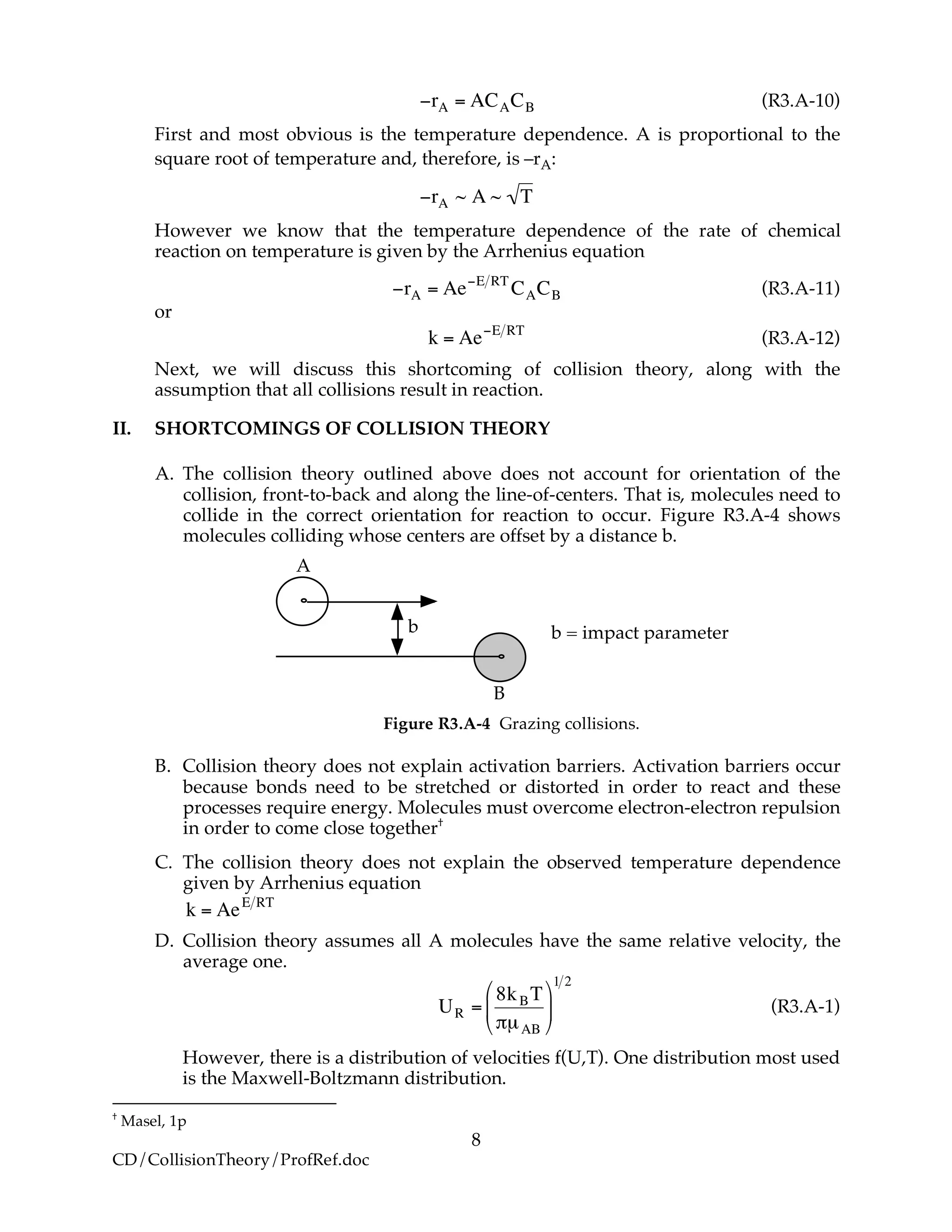
III. MODIFICATIONS OF COLLISION THEORY
We are now going to account for the fact that we have (1) a distribution of relative
velocities UR and (2) that not all collisions only those collisions with an energy EA
or greater result in a reaction--the goal is to arrive at
!
k = Ae"EA RT
A. Distribution of Velocities
We will use the Maxwell-Boltzmann Distribution of Molecular Velocities
(A6p.26). For a species of mass m, the Maxwell distribution of velocities
(relative velocities) is
!
f U,T( )dU = 4"
m
2"kBT
#
$
%
&
'
(
3 2
e)mU2
2kBT
U2
dU (R3.A-13)
A plot of the distribution function, f(U,T), is shown as a function of U in Figure
R3.A-5.
!
f U,T( )f
T1
T2
T2!>!T1
U
Figure R3.A-5 Maxwell-Boltzmann distribution of velocities.
Replacing m by the reduced mass µ of two molecules A and B
!
f U,T( )dU = 4"
µ
2"kBT
#
$
%
&
'
(
3 2
e)µU2
2kBT
U2
dU
The term on the left side of Equation (R3.A-13), [f(U,T)dU], is the fraction of
molecules with velocities between U and (U + dU). Recall from Equation (R3.A-
4) that the number of A–B collisions for a reaction cross section Sr is
!
˜ZAB =Sr U( )U
˜k U( )
123
˜CA
˜CB (R3.A-14)
except now the collision cross-section is a function of the relative velocity.
Note we have written the collision cross section Sr as a function of
velocity U: Sr(U). Why does the velocity enter into reaction cross section, Sr?
Because not all collisions are head on, and those that are not will not react if the
energy (U
2
/2µ) is not sufficiently high. Consequently, this functionality,
Sr = Sr(U), is reasonable because if two molecules collide with a very very low
relative velocity it is unlikely that such a small transfer of kinetic energy is
likely to activate the internal vibrations of the molecule to cause the breaking of
bonds. On the other hand, for collisions with large relative velocities most
collisions will result in reaction.](https://image.slidesharecdn.com/collisiontheory-160829145444/75/Collision-theory-9-2048.jpg)
![10
CD/CollisionTheory/ProfRef.doc
We now let
!
˜k(U) be the specific reaction rate for a collision and reaction
of A-B molecules with a velocity U.
!
˜k U( )=Sr U( )U m3
molecule s[ ] (R3.A-15)
Equation (R3.A-15) will give the specific reaction rate and hence the reaction
rate for only those collisions with velocity U. We need to sum up the collisions
of all velocities. We will use the Maxwell-Boltzmann distribution for f(U,T) and
integrate over all relative velocities.
!
˜k T( )= k0
"
# U( )f(U,T)dU = f U,T( )0
"
# Sr U( ) UdU (R3.A-16)
Maxwell distribution function of velocities for the A/B pair of reduced mass
µAB is†
!
f U,T( )= 4"
µ
2"kBT
#
$
%
&
'
(
3 2
U2
e
)
µU2
2kBT
(R3.A-17)
Combining Equations (16) and (17)
!
˜k T( )= Sr0
"
# U 4$
µ
2$kBT
%
&
'
(
)
*
3 2
U2
e
+
µU2
2kBT
dU (R3.A-18)
For brevity, we let Sr=Sr(U), we will now express the distribution function in
terms of the translational energy εT.
We are now going to express the equation for
!
˜k(T) in terms of kinetic
energy rather than velocity. Relating the differential translational kinetic
energy, ε , to the velocity U:
!t =
µU2
2
Multiplying and dividing by
2
µ
and µ, we obtain
!
d"t =µ UdU
and hence, the reaction rate
!
˜k T( )= 4"
µ
2"kBT
#
$
%
&
'
(
3 2
Sr0
)
*
2
µ
µU2
2
e
+
µU2
2
1
kBT
#
$
%
&
'
(
1
µ
#
$
%
&
'
( µUdU
dµU2
2
d,t
123
123
Simplifying
!
= 4"
µ
2"kBT
#
$
%
&
'
(
3 2
2
µ2
Sr0
)
* +t e
,
+t
kBT
d+t
†
2p185, A5p36](https://image.slidesharecdn.com/collisiontheory-160829145444/75/Collision-theory-10-2048.jpg)
![11
CD/CollisionTheory/ProfRef.doc
!
˜k T( )=
8
"µ kBT( )
3
#
$
%
%
&
'
(
(
1 2
Sr0
)
* +t e
,
+t
kBT
d+t m3
s molecule[ ] (R3.A-19)
!
˜k T( )=
8
"µ kBT( )
3
#
$
%
%
&
'
(
(
1 2
Sr )t( )0
*
+ )t e,)t kBT
d)t
Multiplying and dividing by kBT and noting
!
"t kBT( )= E RT( ), we obtain
!
˜k T( )=
8kBT
"µ
#
$
%
&
'
(
1 2
Sr E( )0
)
*
Ee+E RT
RT
dE
RT
,
-
.
/
0
1 (R3.A-20)
Again, recall the tilde, e.g.,
!
˜k(T), denotes that the specific reaction rate is per
molecule (dm
3
/molecule/s). The only thing left to do is to specify the reaction
cross-section, Sr(E), as a function of kinetic energy E for the A/B pair of
molecules.
B. Collisions that Result in Reaction
We now modify the hard sphere collision cross section to account for the fact
that not all collisions result in reaction. Now we define Sr to be the reaction
cross section defined as
Sr = Pr!"AB
2
where Pr is the probability of reaction. In the first model we say the probability
is either 0 or 1. In the second model Pr varies from 0 to 1 continuously. We will
now insert each of these modules into Equation (R3.A-20).
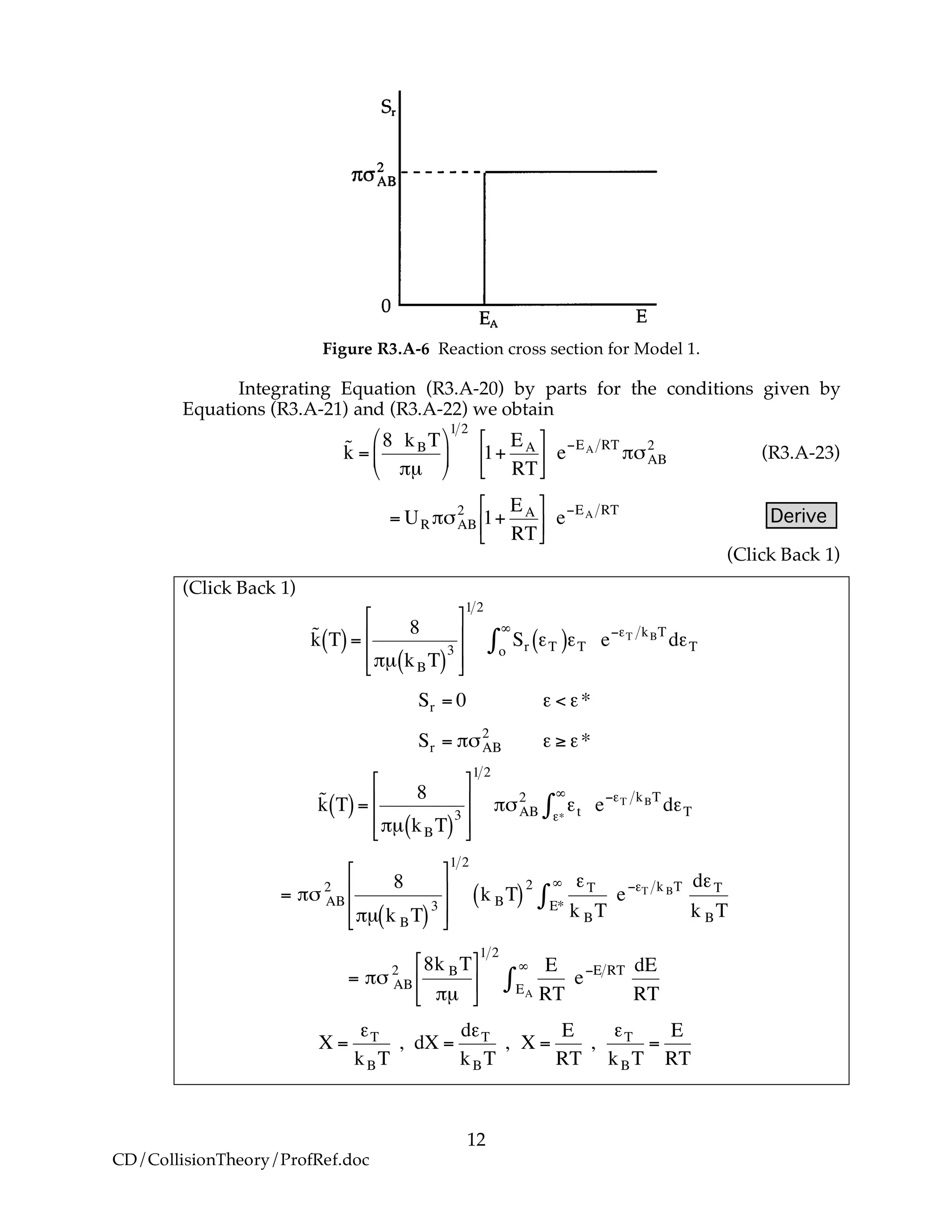
B.1 Model 1
In this model, we say only those hard collisions that have kinetic energy EA or
greater will react. Let E ≡ εt. That is, below this energy, EA, the molecules do not
have sufficient energy to react so the reaction cross section is zero, Sr=0. Above
this kinetic energy all the molecules that collide react and the reaction cross-
section is
!
Sr = "#AB
2
!
Pr = 0" Sr E,T[ ] = 0 for E < EA
Pr =1 Sr E,T[ ] = #$AB
2
for E % EA
(R3.A-21)
(R3.A-22)](https://image.slidesharecdn.com/collisiontheory-160829145444/75/Collision-theory-11-2048.jpg)
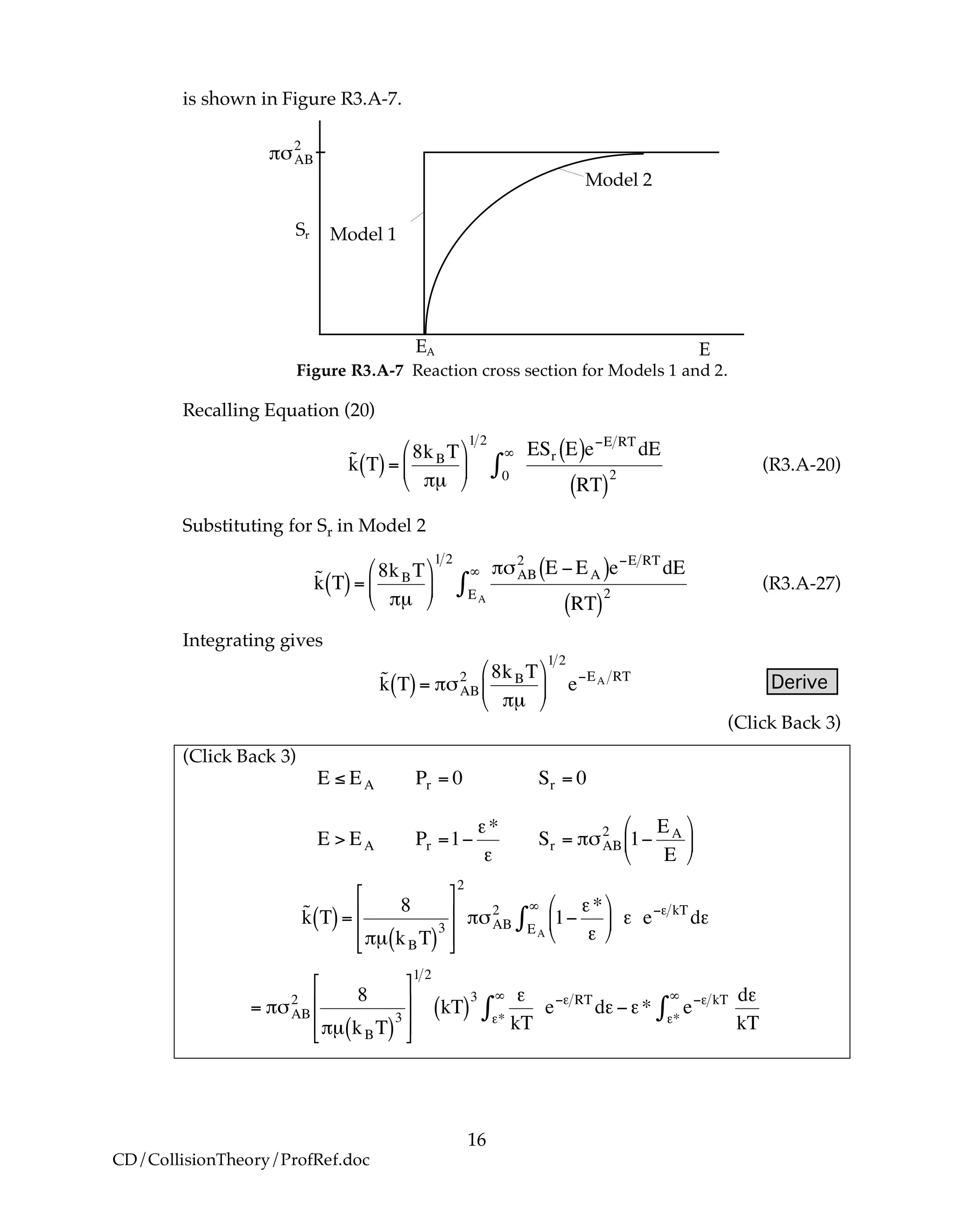
![15
CD/CollisionTheory/ProfRef.doc
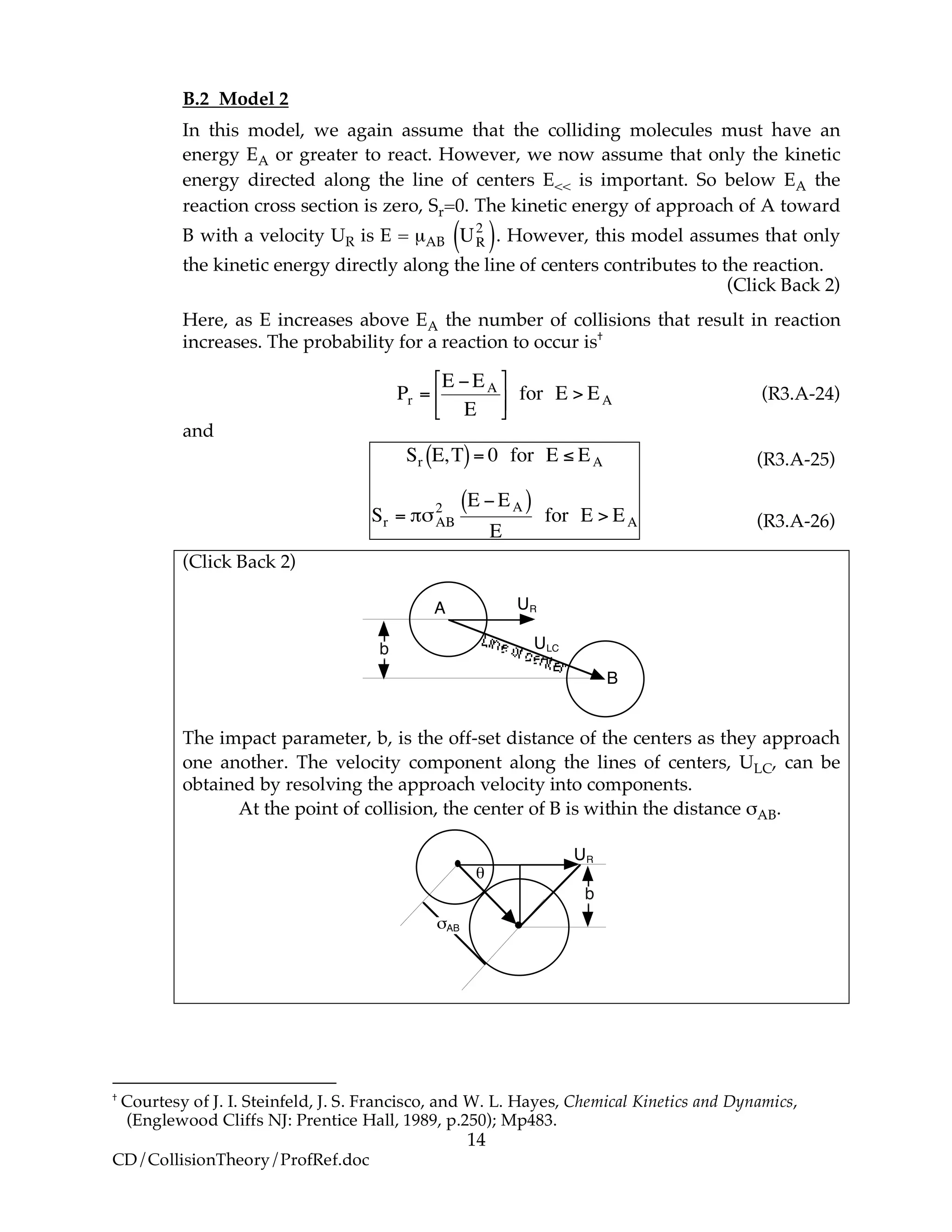
(Click Back 2 cont’d)
The energy along the line of centers can be developed by a simple geometry
argument
!
sin " =
b
#AB
(1)
The component of velocity along the line of centers
ULC = UR cos θ (2)
The kinetic energy along the line of centers is
!
ELC =
ULC
2
µAB
=
UR
2
µAB
cos2
" = E cos2
" (3)
!
ELC = E 1"sin2
#[ ]= E 1"
b2
$AB
2
%
&
'
(
)
* (4)
The minimum energy along the line of centers necessary for a reaction to take
place, EA, corresponds to a critical value of the impact parameter, bcrit. In fact,
this is a way of defining the impact parameter and corresponding reaction
cross section
!
Sr = "bcrit
2
(5)
Substituting for EA and bcrit in Equation (4)
!
EA = E 1"
bcrit
2
#AB
2
$
%
&
'
(
) (6)
Solving for
!
bcrit
2
!
bcr
2
= "AB
2
1#
EA
E
$
%
&
'
(
) (7)
The reaction cross section for energies of approach, E > EA, is
!
Sr = "bcrit
2
= "#AB
2
1$
EA
E
%
&
'
(
)
* (8)
The complete reaction cross section for all energies E is
!
Sr = 0 E " EA
Sr = #$AB
2
1%
EA
E
&
'
(
)
*
+ E > EA
!
(9)
(10)
A plot of the reaction cross section as a function of the kinetic energy of
approach
!
E =µAB
UR
2
2](https://image.slidesharecdn.com/collisiontheory-160829145444/75/Collision-theory-15-2048.jpg)
![21
CD/CollisionTheory/ProfRef.doc
Figure R3.A-10 Experimental correlation of EA and ΔHRx. Courtesy of R. I. Masel,
Chemical Kinetics and Catalysis (New York: Wiley Interscience, 2001).
For this family of reactions
!
EA =12 kcal mol+0.5 "HR (R3.A-34)
For example, when the exothermic heat of reaction is
!
"HRx = #10 kcal mol
The corresponding activation energy is
!
Ea = 7cal mol
To develop the Polyani equation, we consider the elementary exchange reaction†
!
A+BC " AB+C
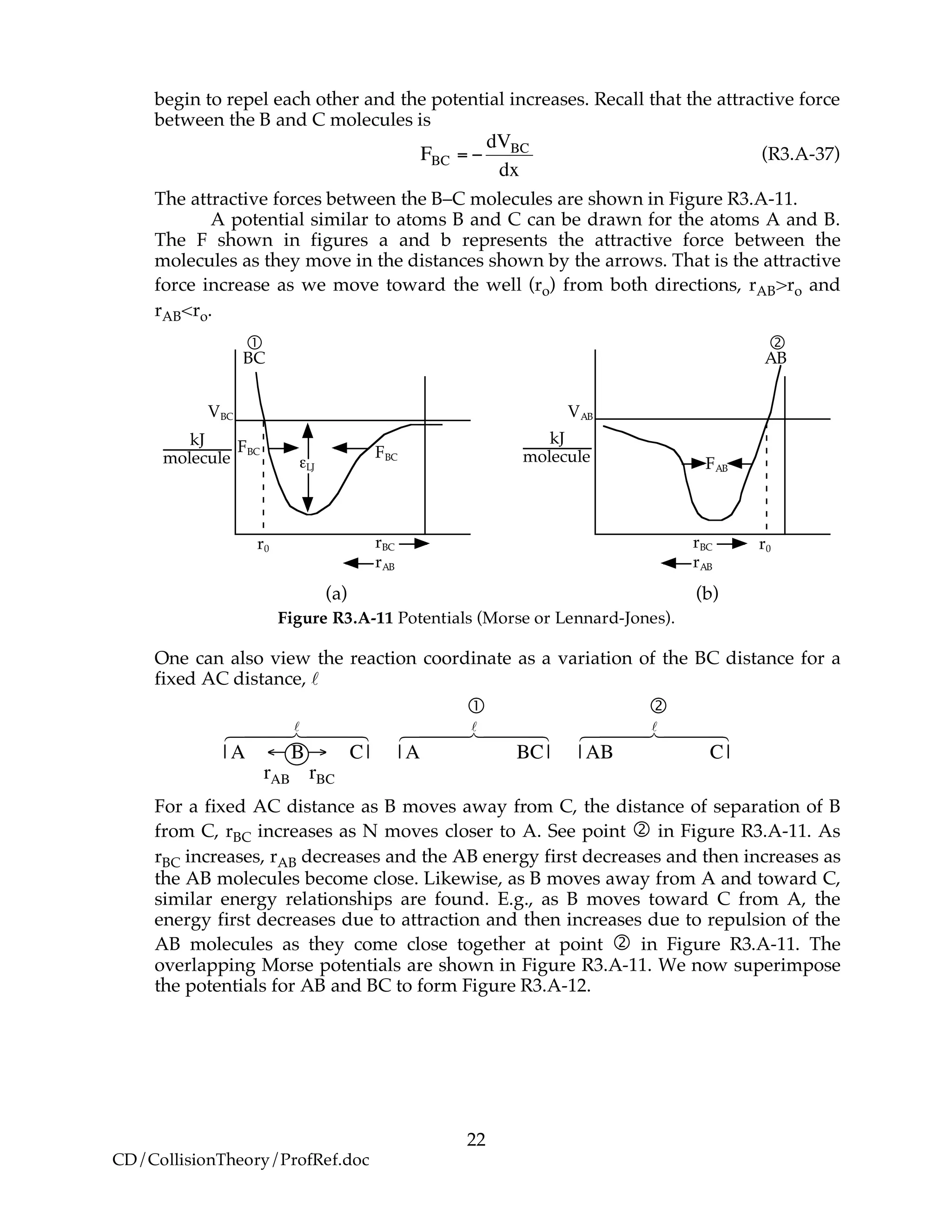
We consider the superposition of two attraction/repulsion potentials, VBC and
VAB, similar to the Lennard-Jones 6-12 potential. For the molecules BC, the
Lennard-Jones potential is
!
VBC = 4"LJ
r0
rBC
#
$
%
&
'
(
12
)
r0
rBC
#
$
%
&
'
(
6*
+
,
,
-
.
/
/
(R3.A-35)
where rBC = distance between molecules (atoms) B and C.
In addition to the Lennard-Jones 6-12 model, another model often used is
the Morse potential, which has a similar shape
VBC = D e
!2" rBC !r0( )
! 2e
!" rBC !r0( )
[ ] (R3.A-36)
When the molecules are far apart the potential V (i.e., Energy) is zero. As
they move closer together, they become attracted to one another and the potential
energy reaches a minimum. As they are brought closer together, the BC molecules
†
After R. I. Masel (Loc cit).](https://image.slidesharecdn.com/collisiontheory-160829145444/75/Collision-theory-21-2048.jpg)
![23
CD/CollisionTheory/ProfRef.doc
Reference
Energy
rBC rAB
E1R
E2P
!HRx=E2P – E1P
r2
r1
BC S2
S1
AB
Ea
rBC = rAB
r*
* *
Reaction Coordinate
Figure R3.A-12 Overlap of potentials (Morse or Lennard-Jones).
Let S1 be the slope of the BC line between r1 and rBC=rAB. Starting at E1R at r1, the
energy E1 at a separation distance of rBC from r1 can be calculated from the product
of the slope S1 and the distance from E1R. The energy, E1, of the BC molecule at any
position rBC relative to r1 is
!
E1 = E1R +S1 rBC " r1( ) (R3.A-38)
!
e.g., E1 = "50kJ+
10kJ
nm
# 5 "2[ ]nm = "20kJ
$
%&
'
()
Let S2 be the slope of the AB line between r2 and rBC=rAB. Similarly for AB, starting
on the product side at E2P, the energy E2 at any position rAB relative to r2 is
!
E2 = E2P +S2 rAB " r2( ) (R3.A-39)
!
e.g., E2 = "80kJ+ "
20kJ
nm
#
$
%
&
'
() 7 "10( )nm = "20kJ
*
+
,
-
.
/
At the height of the barrier
!
E1
"
= E2
"
at rBC
"
= rAB
"
(R3.A-40)
Substituting for
!
E1
"
and
!
E2
"
!
E1R +S1 rBC
"
# r1( )= E2P +S2 rAB
"
# r2( ) (R3.A-41)
Rearranging
!
S1 rBC
"
# r1( )= E2P #E1R( )
$HRx
1 24 34
+S2 rAB
"
# r2( ) (R3.A-42)](https://image.slidesharecdn.com/collisiontheory-160829145444/75/Collision-theory-23-2048.jpg)
![25
CD/CollisionTheory/ProfRef.doc
Recalling Equation (R3.A-43)
!
Ea = E1
"
# E1R = S1 r"
# r1( ) (R3.A-43)
Substituting Equation (C) for r* in Equation (R3.A-43)
!
Ea =S1
"HRx
S1 #S2
+
S1r1 #S2r2
S1 #S2
$
%
&
'
(
)#S1r1 (E)
Rearranging
!
Ea =
S1
S1 "S2
#
$
%
&
'
()HRx +S1
S1r1 "S2r2
S1 "S2
" r1
*
+
,
-
.
/ (F)
!
=
S1
S1 "S2
#
$
%
&
'
()HRx +S1
S1r1 "S2r2 "S1r1 +S2r1
S1 "S2
*
+
,
-
.
/ (G)
Finally, collecting terms we have
!
Ea =
S1
S1 "S2
#
$
%
&
'
(
)P
1 24 34
*HRx +
S1S2
S1 "S2
#
$
%
&
'
( r1 " r2[ ]
Ea
+
1 244 344
(H)
Note: S1 is positive, S2 is negative, and r2 > r1; therefore, Ea
!
is positive, as is
γP.
Ea = Ea
!
+ " p#HRx
B. Marcus Extension of the Polyani Equation
In reasoning similar to developing the Polyani Equation, Marcus shows (see
Masel, pp. 584-586)
!
EA = 1+
"HRx
4EA0
#
$
%
&
'
(
2
EA0
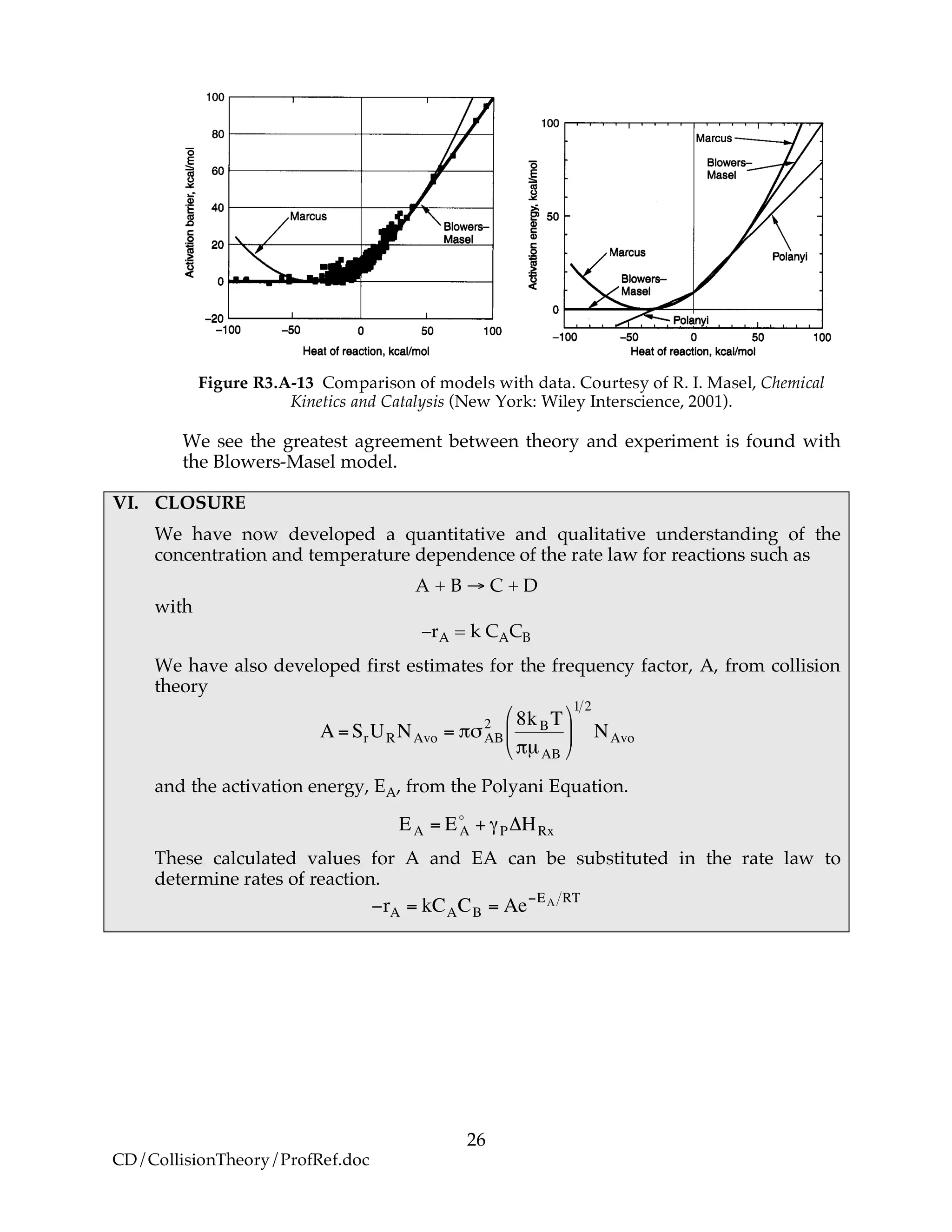
C. Blowers-Masel Relation
The Polyani Equation will predict negative activation energies for highly
exothermic reactions. Blowers and Masel developed a relationship that
compares quite well with experiments throughout the entire range of heat of
reaction for the family of reactions
!
R +H "R # RH + "R
as shown in Figure R3.A-13.](https://image.slidesharecdn.com/collisiontheory-160829145444/75/Collision-theory-25-2048.jpg)
![27
CD/CollisionTheory/ProfRef.doc
VI. OTHER STUFF
Potential Energy Surfaces and the barrier height εhb
Figure R3.A-14 Reaction coordinates.
The average transitional energy of a molecule undergoing collision is 2kBT.
The molecules with a higher energy are more likely to collide.
A. How to Calculate Barrier Height
(1) Ab Initio calculations. No adjustment of parameters or use of experimental
data.
Solve Schrödinger’s Equation
Eb = Barrier Height ≡ εhb
Eb = 40 kJ/mol for the H + H2 exchange reaction
(2) Semiempirical
Uses experimental measurements (spectroscopic).
Adjustments are made to get agreement.
(3) London-Eyring-Polanyi (LEP) Method
(LEP) Surface
Use spectroscopic measurement in conjunction with the Morse potential
equation
E = D e
!2" r!r0( )
! 2 e
!" r !r0( )
[ ]
D = dissociation energy
ro = equilibrium internuclear distance
β = constant
Model B3 Stored Energy
This third method considers vibrational and translation energy in addition to
translational energy. Even though this approach is oversimplified, it is
satisfying because it gives a qualitative feel for the Arrhenius temperature
dependence. In this approach, we say the fraction of molecules that will react
are those that have acquired an energy EA.](https://image.slidesharecdn.com/collisiontheory-160829145444/75/Collision-theory-27-2048.jpg)

Collision theory provides a qualitative understanding of reaction rate laws. It models reactant molecules as rigid spheres and calculates the collision rate based on their concentrations and relative velocities. However, collision theory has shortcomings. It predicts a temperature dependence of the rate constant proportional to the square root of temperature, rather than the exponential dependence seen in the Arrhenius equation. It also assumes all collisions result in reaction, overestimating reaction rates. Modifications are needed to account for a distribution of collision energies and the fact that only collisions above an activation energy can react.