Download free for 30 days
Sign in
Upload
Language (EN)
Support
Business
Mobile
Social Media
Marketing
Technology
Art & Photos
Career
Design
Education
Presentations & Public Speaking
Government & Nonprofit
Healthcare
Internet
Law
Leadership & Management
Automotive
Engineering
Software
Recruiting & HR
Retail
Sales
Services
Science
Small Business & Entrepreneurship
Food
Environment
Economy & Finance
Data & Analytics
Investor Relations
Sports
Spiritual
News & Politics
Travel
Self Improvement
Real Estate
Entertainment & Humor
Health & Medicine
Devices & Hardware
Lifestyle
Change Language
Language
English
Español
Português
Français
Deutsche
Cancel
Save
Submit search
EN
Uploaded by
MehediHasanRidoy4
PDF, PPTX
28 views
Classification Algorithm in Big Data.pdf
Classification algorithm is a algorithm of machine learning
Education
◦
Read more
0
Save
Share
Embed
Embed presentation
Download
Download as PDF, PPTX
1
/ 63
2
/ 63
3
/ 63
Most read
4
/ 63
5
/ 63
6
/ 63
7
/ 63
8
/ 63
9
/ 63
10
/ 63
11
/ 63
12
/ 63
13
/ 63
14
/ 63
15
/ 63
16
/ 63
17
/ 63
18
/ 63
19
/ 63
20
/ 63
21
/ 63
22
/ 63
23
/ 63
24
/ 63
25
/ 63
26
/ 63
27
/ 63
28
/ 63
29
/ 63
30
/ 63
31
/ 63
32
/ 63
33
/ 63
34
/ 63
35
/ 63
36
/ 63
37
/ 63
38
/ 63
39
/ 63
40
/ 63
41
/ 63
42
/ 63
43
/ 63
44
/ 63
45
/ 63
46
/ 63
47
/ 63
48
/ 63
49
/ 63
50
/ 63
51
/ 63
52
/ 63
53
/ 63
54
/ 63
55
/ 63
56
/ 63
57
/ 63
58
/ 63
59
/ 63
60
/ 63
61
/ 63
62
/ 63
63
/ 63
More Related Content
PPTX
Machine learning and decision trees
by
Padma Metta
PDF
An Introduction to Supervised Machine Learning and Pattern Classification: Th...
by
Sebastian Raschka
PPT
[ppt]
by
butest
PPT
[ppt]
by
butest
PDF
wzhu_paper
by
Wenzhen Zhu
PDF
IRJET- Performance Evaluation of Various Classification Algorithms
by
IRJET Journal
PDF
IRJET- Performance Evaluation of Various Classification Algorithms
by
IRJET Journal
PDF
MLHEP 2015: Introductory Lecture #1
by
arogozhnikov
Machine learning and decision trees
by
Padma Metta
An Introduction to Supervised Machine Learning and Pattern Classification: Th...
by
Sebastian Raschka
[ppt]
by
butest
[ppt]
by
butest
wzhu_paper
by
Wenzhen Zhu
IRJET- Performance Evaluation of Various Classification Algorithms
by
IRJET Journal
IRJET- Performance Evaluation of Various Classification Algorithms
by
IRJET Journal
MLHEP 2015: Introductory Lecture #1
by
arogozhnikov
Similar to Classification Algorithm in Big Data.pdf
PPTX
UNIT 3: Data Warehousing and Data Mining
by
Nandakumar P
PDF
Machine Learning: Classification Concepts (Part 1)
by
Daniel Chan
PPTX
Data Mining Lecture_10(b).pptx
by
Subrata Kumer Paul
PPTX
Deep learning from mashine learning AI..
by
premkumarlive
PPT
Introduction to Machine Learning Aristotelis Tsirigos
by
butest
PDF
Linear models for classification
by
Sung Yub Kim
PPTX
BAS 250 Lecture 8
by
Wake Tech BAS
PPTX
Module 1 Taxonomy of Machine L(1).pptx
by
angelinjeba6
PPTX
Unit 4 Classification of data and more info on it
by
randomguy1722
PPT
Business Analytics using R.ppt
by
Rohit Raj
PDF
lec6_annotated.pdf ml csci 567 vatsal sharan
by
agrimsachdeva2
PPT
594503964-Introduction-to-Classification-PPT-Slides-1.ppt
by
snehajuly2004
PDF
01_CS115 Machine Learning Overview .pdf
by
NguynTrngNhn42
PDF
Presentation-19.08.2024hvug7gugyvuvugugugugugug
by
amanna7980
PPTX
Svm my
by
Subhadeep Karan
PPT
Category vectorspaceessex
by
Shishir Kakaraddi
PDF
Data Science Cheatsheet.pdf
by
qawali1
PDF
machine_learning.pptx
by
Panchami V U
PPTX
Svm my
by
Subhadeep Karan
PPT
Machine learning by Dr. Vivek Vijay and Dr. Sandeep Yadav
by
Agile Testing Alliance
UNIT 3: Data Warehousing and Data Mining
by
Nandakumar P
Machine Learning: Classification Concepts (Part 1)
by
Daniel Chan
Data Mining Lecture_10(b).pptx
by
Subrata Kumer Paul
Deep learning from mashine learning AI..
by
premkumarlive
Introduction to Machine Learning Aristotelis Tsirigos
by
butest
Linear models for classification
by
Sung Yub Kim
BAS 250 Lecture 8
by
Wake Tech BAS
Module 1 Taxonomy of Machine L(1).pptx
by
angelinjeba6
Unit 4 Classification of data and more info on it
by
randomguy1722
Business Analytics using R.ppt
by
Rohit Raj
lec6_annotated.pdf ml csci 567 vatsal sharan
by
agrimsachdeva2
594503964-Introduction-to-Classification-PPT-Slides-1.ppt
by
snehajuly2004
01_CS115 Machine Learning Overview .pdf
by
NguynTrngNhn42
Presentation-19.08.2024hvug7gugyvuvugugugugugug
by
amanna7980
Svm my
by
Subhadeep Karan
Category vectorspaceessex
by
Shishir Kakaraddi
Data Science Cheatsheet.pdf
by
qawali1
machine_learning.pptx
by
Panchami V U
Svm my
by
Subhadeep Karan
Machine learning by Dr. Vivek Vijay and Dr. Sandeep Yadav
by
Agile Testing Alliance
Recently uploaded
PDF
Application of ICT Lecture 7 Ethical Considerations in Use of ICT Platforms a...
by
Khalil Khan Marwat
PPTX
Chapter No. 5 Anti- Hypertensive Pharmacognosy-2.pptx
by
Ganu Gavade
PPTX
Cardiovascular System or The Details of Heart.pptx
by
Ashish Umale
PDF
Enhancing Accessibility and Inclusivity: The TU Dublin Leaving Certificate St...
by
CONUL Conference
PPTX
LEARNING PART 1. SHILPA HOTAKAR PSYCHOLOGY NOTES pptx
by
SHILPA HOTAKAR
PDF
Sentence Comprehension The Integration of Habits and Rules (Language, Speech,...
by
Man_Ebook
PDF
PROBLEM SLOVING AND PYTHON PROGRAMMING Unit 1.pdf
by
A R SIVANESH M.E., (Ph.D)
PDF
BỘ 20 ĐỀ THI GIẢ LẬP MỨC ĐỘ 9+ KỲ THI TỐT NGHIỆP TRUNG HỌC PHỔ THÔNG NĂM 2026...
by
Nguyen Thanh Tu Collection
PDF
A predictive coding framework for rapid neural dynamics during sentence-level...
by
Man_Ebook
PPTX
Auto Plan Feature in Odoo 18 Planning Module
by
Celine George
PDF
Visualising Library Insights: Power BI Dashboard for Data-Driven Decision Mak...
by
CONUL Conference
PPTX
Set online status in Odoo 19_Do not distrurb
by
Celine George
PDF
Generative AI and Bibliographic Record Generation: Reflections on Experiments...
by
CONUL Conference
PPTX
Caring for Collections – New directions at UCC Library. Louise O’Connor, Uni...
by
CONUL Conference
PPTX
‘Guiding the AI Generation, Are Librarians the Missing Link?’ Speaker: Rob Mo...
by
CONUL Conference
PPTX
SPECIAL STSAINS USED IN HISTOPATHOLOGY.pptx
by
KISMAT ALI
PPTX
Conduction System of the Heart, The Cardiac Cycle, The Cardiac Output, ECG.pptx
by
Ashish Umale
PPTX
From Vision to Action: UCC Library’s Digital & Information Literacy Framework...
by
CONUL Conference
PPTX
AI Literacy at UCD Library. Dr Marta Bustillo & Sandra Dunkin, University Col...
by
CONUL Conference
PDF
The Scientific Research Lifecycle From Concept to Publication.pdf
by
Muhammad Fahad Bashir
Application of ICT Lecture 7 Ethical Considerations in Use of ICT Platforms a...
by
Khalil Khan Marwat
Chapter No. 5 Anti- Hypertensive Pharmacognosy-2.pptx
by
Ganu Gavade
Cardiovascular System or The Details of Heart.pptx
by
Ashish Umale
Enhancing Accessibility and Inclusivity: The TU Dublin Leaving Certificate St...
by
CONUL Conference
LEARNING PART 1. SHILPA HOTAKAR PSYCHOLOGY NOTES pptx
by
SHILPA HOTAKAR
Sentence Comprehension The Integration of Habits and Rules (Language, Speech,...
by
Man_Ebook
PROBLEM SLOVING AND PYTHON PROGRAMMING Unit 1.pdf
by
A R SIVANESH M.E., (Ph.D)
BỘ 20 ĐỀ THI GIẢ LẬP MỨC ĐỘ 9+ KỲ THI TỐT NGHIỆP TRUNG HỌC PHỔ THÔNG NĂM 2026...
by
Nguyen Thanh Tu Collection
A predictive coding framework for rapid neural dynamics during sentence-level...
by
Man_Ebook
Auto Plan Feature in Odoo 18 Planning Module
by
Celine George
Visualising Library Insights: Power BI Dashboard for Data-Driven Decision Mak...
by
CONUL Conference
Set online status in Odoo 19_Do not distrurb
by
Celine George
Generative AI and Bibliographic Record Generation: Reflections on Experiments...
by
CONUL Conference
Caring for Collections – New directions at UCC Library. Louise O’Connor, Uni...
by
CONUL Conference
‘Guiding the AI Generation, Are Librarians the Missing Link?’ Speaker: Rob Mo...
by
CONUL Conference
SPECIAL STSAINS USED IN HISTOPATHOLOGY.pptx
by
KISMAT ALI
Conduction System of the Heart, The Cardiac Cycle, The Cardiac Output, ECG.pptx
by
Ashish Umale
From Vision to Action: UCC Library’s Digital & Information Literacy Framework...
by
CONUL Conference
AI Literacy at UCD Library. Dr Marta Bustillo & Sandra Dunkin, University Col...
by
CONUL Conference
The Scientific Research Lifecycle From Concept to Publication.pdf
by
Muhammad Fahad Bashir
Classification Algorithm in Big Data.pdf
1.
Statistical Learning for
Big Data Chapter 3.2: Supervised Learning — Classification
2.
Classification Tasks A. Marx,
P. Bürkner © winter term 24/25 Statistical Learning for Big Data – 2 / 63
3.
CLASSIFICATION Learn functions that
assign class labels to observation / feature vectors. Each observation belongs to exactly one class. The main difference to regression is the scale of the output / label. Sepal Length Sepal Width Petal Length Petal Width Species 5.1 3.5 1.4 0.2 setosa 5.9 3.0 5.1 1.8 virginica Classifier Sepal Length Sepal Width Petal Length Petal Width Species 5.4 3.3 3.2 1.1 ??? New Data with unknown label New Class label Our Data A. Marx, P. Bürkner © winter term 24/25 Statistical Learning for Big Data – 3 / 63
4.
BINARY AND MULTICLASS
TASKS The task can contain two (binary) or multiple (multiclass) classes. 0.00 0.05 0.10 0.15 0.20 0.00 0.01 0.02 0.03 0.04 0.05 V1 V2 Response M R Sonar 0.0 0.5 1.0 1.5 2.0 2.5 2 4 6 Petal.Length Petal.Width Response setosa versicolor virginica Iris A. Marx, P. Bürkner © winter term 24/25 Statistical Learning for Big Data – 4 / 63
5.
BINARY CLASSIFICATION TASK
- EXAMPLES Credit risk prediction, based on personal data and transactions Spam detection, based on textual features Churn prediction, based on customer behavior Predisposition for specific illness, based on genetic data https://www.bendbulletin.com/localstate/deschutescounty/3430324-151/fact-or-fiction-polygraphs-just-an-investigative-tool A. Marx, P. Bürkner © winter term 24/25 Statistical Learning for Big Data – 5 / 63
6.
MULTICLASS TASK -
IRIS The iris dataset was introduced by the statistician Ronald Fisher and is one of the most frequently used data sets. Originally, it was designed for linear discriminant analysis. Setosa Versicolor Virginica Source: https://en.wikipedia.org/wiki/Iris_flower_data_set A. Marx, P. Bürkner © winter term 24/25 Statistical Learning for Big Data – 6 / 63
7.
MULTICLASS TASK -
IRIS 150 iris flowers Predict subspecies Based on sepal and petal length / width in [cm] ## Sepal.Length Sepal.Width Petal.Length Petal.Width Species ## 1: 5.1 3.5 1.4 0.2 setosa ## 2: 4.9 3.0 1.4 0.2 setosa ## 3: 4.7 3.2 1.3 0.2 setosa ## 4: 4.6 3.1 1.5 0.2 setosa ## 5: 5.0 3.6 1.4 0.2 setosa ## --- ## 146: 6.7 3.0 5.2 2.3 virginica ## 147: 6.3 2.5 5.0 1.9 virginica ## 148: 6.5 3.0 5.2 2.0 virginica ## 149: 6.2 3.4 5.4 2.3 virginica ## 150: 5.9 3.0 5.1 1.8 virginica A. Marx, P. Bürkner © winter term 24/25 Statistical Learning for Big Data – 7 / 63
8.
MULTICLASS TASK -
IRIS Corr: −0.118 setosa: 0.743*** versicolor: 0.526*** virginica: 0.457*** Corr: 0.872*** setosa: 0.267. versicolor: 0.754*** virginica: 0.864*** Corr: −0.428*** setosa: 0.178 versicolor: 0.561*** virginica: 0.401** Corr: 0.818*** setosa: 0.278. versicolor: 0.546*** virginica: 0.281* Corr: −0.366*** setosa: 0.233 versicolor: 0.664*** virginica: 0.538*** Corr: 0.963*** setosa: 0.332* versicolor: 0.787*** virginica: 0.322* Sepal.Length Sepal.Width Petal.Length Petal.Width Species Sepal.Length Sepal.Width Petal.Length Petal.Width Species 5 6 7 8 2.0 2.5 3.0 3.5 4.0 4.5 2 4 6 0.0 0.5 1.0 1.5 2.0 2.5 setosaversicolor virginica 0.0 0.4 0.8 1.2 2.0 2.5 3.0 3.5 4.0 4.5 2 4 6 0.0 0.5 1.0 1.5 2.0 2.5 0.0 2.5 5.0 7.5 0.0 2.5 5.0 7.5 0.0 2.5 5.0 7.5 A. Marx, P. Bürkner © winter term 24/25 Statistical Learning for Big Data – 8 / 63
9.
Basic Definitions A. Marx,
P. Bürkner © winter term 24/25 Statistical Learning for Big Data – 9 / 63
10.
CLASSIFICATION TASKS In a
classification task, we aim at predicting a discrete output y ∈ Y = {C1, ..., Cg} with 2 ≤ g < ∞, given data D. In this course, we assume the classes to be encoded as Y = {0, 1} or Y = {−1, +1} (in the binary case g = 2) Y = {1, . . . , g} (in the multiclass case g ≥ 3) A. Marx, P. Bürkner © winter term 24/25 Statistical Learning for Big Data – 10 / 63
11.
CLASSIFICATION MODELS We define
models f : X → Rg as functions that output (continuous) scores / probabilities but not (discrete) classes. Why? From an optimization perspective, it is much (!) easier to optimize costs for continuous-valued functions Scores / probabilities (for classes) contain more information than the class labels alone As we will see later, scores can easily be transformed into class labels; but class labels cannot be transformed into scores We distinguish scoring and probabilistic classifiers. A. Marx, P. Bürkner © winter term 24/25 Statistical Learning for Big Data – 11 / 63
12.
SCORING CLASSIFIERS Construct g
discriminant / scoring functions f1, ..., fg : X → R Scores f1(x), . . . , fg(x) are transformed into classes by choosing the class attaining the maximum score h(x) = arg max k∈{1,...,g} fk (x). Consider g = 2: A single discriminant function f(x) = f1(x) − f−1(x) is sufficient (assuming the class labels {−1, +1}) Class labels are constructed by h(x) = sgn(f(x)) |f(x)| is called confidence A. Marx, P. Bürkner © winter term 24/25 Statistical Learning for Big Data – 12 / 63
13.
PROBABILISTIC CLASSIFIERS Construct g
probability functions π1, ..., πg : X → [0, 1] with the constraint that P i πi = 1 Probabilities π1(x), . . . , πg(x) are transformed into labels by predicting the class attaining the maximum probability h(x) = arg max k∈{1,...,g} πk (x) For g = 2, one π(x) is sufficient for labels {0, 1} Note that: Probabilistic classifiers can also be seen as scoring classifiers If we want to emphasize that our model outputs probabilities, we denote the model as π(x) : X → [0, 1]g . When talking about models in general, we write f, comprising both probabilistic and scoring classifiers, which will become clear from the context! A. Marx, P. Bürkner © winter term 24/25 Statistical Learning for Big Data – 13 / 63
14.
CLASSIFIERS: THRESHOLDING Both, scoring
and probabilistic classifiers, can output classes by thresholding (binary case) / selecting the class attaining the maximum score (multiclass) Given a threshold c: h(x) := [f(x) ≥ c] Usually c = 0.5 for probabilistic, c = 0 for scoring classifiers There are also versions of thresholding for the multiclass case A. Marx, P. Bürkner © winter term 24/25 Statistical Learning for Big Data – 14 / 63
15.
DECISION REGIONS AND
BOUNDARIES A decision region for class k is the set of input points x where class k is assigned as prediction of our model: Xk = {x ∈ X : h(x) = k} Points in space where the classes with maximal score are tied and the corresponding hypersurfaces are called decision boundaries {x ∈ X : ∃ i ̸= j s.t. fi (x) = fj (x) and fi (x), fj (x) ≥ fk (x) ∀k ̸= i, j} In the binary case we can simplify and generalize to the decision boundary for general threshold c: {x ∈ X : f(x) = c} If we set c = 0 for scores and c = 0.5 for probabilities, this is consistent with the definition above. A. Marx, P. Bürkner © winter term 24/25 Statistical Learning for Big Data – 15 / 63
16.
DECISION BOUNDARY EXAMPLES 0.000 0.025 0.050 0.075 0.100 0.00
0.01 0.02 0.03 0.04 0.05 V1 V2 Response M R Log. Regr. 0.000 0.025 0.050 0.075 0.100 0.00 0.01 0.02 0.03 0.04 0.05 V1 V2 Response M R Naive Bayes 0.000 0.025 0.050 0.075 0.100 0.00 0.01 0.02 0.03 0.04 0.05 V1 V2 Response M R CART Tree 0.000 0.025 0.050 0.075 0.100 0.00 0.01 0.02 0.03 0.04 0.05 V1 V2 Response M R SVM A. Marx, P. Bürkner © winter term 24/25 Statistical Learning for Big Data – 16 / 63
17.
CLASSIFICATION APPROACHES Two fundamental
approaches exist to construct classifiers: The generative approach and the discriminant approach. They tackle the classification problem from different angles: Discriminant approaches use empirical risk minimization based on a suitable loss function: “What is the best prediction for y given these x?” Generative classification approaches assume a data-generating process in which the distribution of the features x is different for the various classes of the output y, and try to learn these conditional distributions: “Which y tends to have x like these?” A. Marx, P. Bürkner © winter term 24/25 Statistical Learning for Big Data – 17 / 63
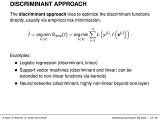
18.
DISCRIMINANT APPROACH The discriminant
approach tries to optimize the discriminant functions directly, usually via empirical risk minimization. f̂ = arg min f∈H Remp(f) = arg min f∈H n X i=1 L y(i) , f x(i) . Examples: Logistic regression (discriminant, linear) Support vector machines (discriminant and linear; can be extended to non-linear functions via kernels) Neural networks (discriminant, highly non-linear beyond one layer) A. Marx, P. Bürkner © winter term 24/25 Statistical Learning for Big Data – 18 / 63
19.
GENERATIVE APPROACH The generative
approach employs Bayes’ theorem and models p(x|y = k) by making assumptions about the structure of these distributions: πk (x) = P(y = k | x) | {z } Posterior = Likelihood z }| { P(x|y = k) Prior z }| { P(y = k) P(x) |{z} Marginal Likelihood = p(x|y = k)πk g P j=1 p(x|y = j)πj Prior class probabilities πk are easy to estimate from the training data. Examples: Naïve Bayes classifier Linear discriminant analysis (generative, linear) Quadratic discriminant analysis (generative, non-linear) Caution: LDA and QDA have ’discriminant’ in their name, but they are generative models! A. Marx, P. Bürkner © winter term 24/25 Statistical Learning for Big Data – 19 / 63
20.
Linear Classifiers A. Marx,
P. Bürkner © winter term 24/25 Statistical Learning for Big Data – 20 / 63
21.
LINEAR CLASSIFIERS Linear classifiers
are an important subclass of classification models. If the discriminant function(s) fk (x) can be specified as linear function(s) (possibly through a rank-preserving, monotonic transformation g : R → R), i. e., g(fk (x)) = w⊤ k x + bk , we will call the classifier a linear classifier. A. Marx, P. Bürkner © winter term 24/25 Statistical Learning for Big Data – 21 / 63
22.
LINEAR CLASSIFIERS We can
show that the decision boundary between classes i and j is a hyperplane. For arbitrary x attaining a tie w.r.t. its scores: fi (x) = fj (x) g(fi (x))) = g(fj (x)) w⊤ i x + bi = w⊤ j x + bj (wi − wj )⊤ x + (bi − bj ) = 0 This specifies a hyperplane separating two classes. A. Marx, P. Bürkner © winter term 24/25 Statistical Learning for Big Data – 22 / 63
23.
LINEAR VS NONLINEAR
DECISION BOUNDARY 2.0 2.5 3.0 3.5 5 6 7 8 Sepal.Length Sepal.Width Response versicolor virginica 2.0 2.5 3.0 3.5 5 6 7 8 Sepal.Length Sepal.Width Response versicolor virginica A. Marx, P. Bürkner © winter term 24/25 Statistical Learning for Big Data – 23 / 63
24.
Logistic Regression A. Marx,
P. Bürkner © winter term 24/25 Statistical Learning for Big Data – 24 / 63
25.
MOTIVATION A discriminant approach
for directly modeling the posterior probabilities π(x | θ) of the labels is logistic regression. For now, let’s focus on the binary case y ∈ {0, 1} and use empirical risk minimization. arg min θ∈Θ Remp(θ) = arg min θ∈Θ n X i=1 L y(i) , π x(i) | θ . A naïve approach would be to model∗ π(x | θ) = θT x. Obviously this could result in predicted probabilities π(x | θ) ̸∈ [0, 1]. ∗ Note: we suppress the intercept for a concise notation. A. Marx, P. Bürkner © winter term 24/25 Statistical Learning for Big Data – 25 / 63
26.
LOGISTIC FUNCTION To avoid
this, logistic regression “squashes” the estimated linear scores θT x to [0, 1] through the logistic function s: π(x | θ) = exp θT x 1 + exp (θT x) = 1 1 + exp (−θT x) = s θT x 0.00 0.25 0.50 0.75 1.00 −10 −5 0 5 10 f s(f) A. Marx, P. Bürkner © winter term 24/25 Statistical Learning for Big Data – 26 / 63
27.
LOGISTIC FUNCTION The intercept
shifts s(f) horizontally s(θ0 + f) = exp(θ0+f) 1+exp(θ0+f) 0.00 0.25 0.50 0.75 1.00 −10 −5 0 5 10 f s(f) θ0 −3 0 3 Scaling f controls the slope and direction of s(αf) = exp(αf) 1+exp(αf). 0.00 0.25 0.50 0.75 1.00 −10 −5 0 5 10 f s(f) α −2 −0.3 1 6 A. Marx, P. Bürkner © winter term 24/25 Statistical Learning for Big Data – 27 / 63
28.
BERNOULLI / LOG
LOSS We need to define a loss function for the ERM approach, and model y | x, θ with as Bernoulli, i. e. p(y | x, θ) = (1 − π(x | θ)) if y = 0, π(x | θ) if y = 1, 0 else. To arrive at the loss function, we consider the negative log-likelihood: L(y, π(x | θ)) = −y ln(π(x | θ)) − (1 − y) ln(1 − π(x | θ)) Also called cross-entropy loss Used for many other classifiers, e.g., neural networks or boosting A. Marx, P. Bürkner © winter term 24/25 Statistical Learning for Big Data – 28 / 63
29.
BERNOULLI / LOG
LOSS Heavy penalty for confidently wrong predictions Recall: L(y, π(x | θ)) = −y ln(π(x | θ)) − (1 − y) ln(1 − π(x | θ)) 0 2 4 6 0.00 0.25 0.50 0.75 1.00 π(x) L ( y, π ( x )) y 0 1 A. Marx, P. Bürkner © winter term 24/25 Statistical Learning for Big Data – 29 / 63
30.
LOGISTIC REGRESSION IN
1D With one feature x ∈ R. The figure shows data and x 7→ π(x). 0.00 0.25 0.50 0.75 1.00 0 2 4 6 x π ( x ) A. Marx, P. Bürkner © winter term 24/25 Statistical Learning for Big Data – 30 / 63
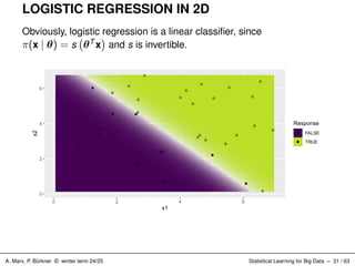
31.
LOGISTIC REGRESSION IN
2D Obviously, logistic regression is a linear classifier, since π(x | θ) = s θT x and s is invertible. 0 2 4 6 0 2 4 6 x1 x2 Response FALSE TRUE A. Marx, P. Bürkner © winter term 24/25 Statistical Learning for Big Data – 31 / 63
32.
LOGISTIC REGRESSION IN
2D 0.00 0.25 0.50 0.75 1.00 −10 −5 0 5 10 score prob A. Marx, P. Bürkner © winter term 24/25 Statistical Learning for Big Data – 32 / 63
33.
SUMMARY OF LOGISTIC
REGRESSION Hypothesis Space: H = π : X → [0, 1] | π(x) = s(θT x) Risk: Logistic/Bernoulli loss function. L (y, π(x)) = −y ln(π(x)) − (1 − y) ln(1 − π(x)) Optimization: Numerical optimization, typically gradient-based methods. A. Marx, P. Bürkner © winter term 24/25 Statistical Learning for Big Data – 33 / 63
34.
Multiclass Classification A. Marx,
P. Bürkner © winter term 24/25 Statistical Learning for Big Data – 34 / 63
35.
FROM LOGISTIC REGRESSION... Recall
logistic regression (Y = {0, 1}): We combined the hypothesis space of linear functions, transformed by the logistic function s(z) = 1 1+exp(−z) H = n π : X → R | π(x) = s(θ⊤ x) o with the Bernoulli (logarithmic) loss: L(y, π(x)) = −y log (π(x)) − (1 − y) log (1 − π(x)) . A. Marx, P. Bürkner © winter term 24/25 Statistical Learning for Big Data – 35 / 63
36.
...TO SOFTMAX REGRESSION There
is a straightforward generalization to the multiclass case: Instead of a single linear discriminant function we have g linear discriminant functions fk (x) = θ⊤ k x, k = 1, 2, ..., g, one for each class. The g score functions are transformed into g probability functions by the softmax function s : Rg → Rg πk (x) = s(f(x))k = exp(θ⊤ k x) Pg j=1 exp(θ⊤ j x) instead of the logistic function for g = 2. The probabilities are well-defined: P πk (x) = 1 and πk (x) ∈ [0, 1] for all k. A. Marx, P. Bürkner © winter term 24/25 Statistical Learning for Big Data – 36 / 63
37.
...TO SOFTMAX REGRESSION The
softmax function is a generalization of the logistic function. For g = 2, they are equivalent. Instead of Bernoulli, we use the multiclass logarithmic loss L(y, π(x)) = − g X k=1 1{y=k} log (πk (x)) . Note that the softmax function is a smooth approximation of the arg max operation, so s((1, 1000, 2)T ) ≈ (0, 1, 0)T (selects 2nd element!). Furthermore, it is invariant to constant offsets in the input: s(f(x)+c) = exp(θ⊤ k x + c) Pg j=1 exp(θ⊤ j x + c) = exp(θ⊤ k x) · exp(c) Pg j=1 exp(θ⊤ j x) · exp(c) = s(f(x)) A. Marx, P. Bürkner © winter term 24/25 Statistical Learning for Big Data – 37 / 63
38.
LOGISTIC VS. SOFTMAX
REGRESSION Logistic Regression Softmax Regression Y {0, 1} {1, 2, ..., g} Discriminant fun. f(x) = θ⊤x fk (x) = θ⊤ k x, k = 1, 2, ..., g Probabilities π(x) = 1 1+exp(−θ⊤x) πk (x) = exp(θ⊤ k x) Pg j=1 exp(θ⊤ j x) L(y, π(x)) Bernoulli / logarithmic loss Multiclass logarithmic loss −y log (π(x)) − (1 − y) log (1 − π(x)) − Pg k=1[y = k] log (πk (x)) A. Marx, P. Bürkner © winter term 24/25 Statistical Learning for Big Data – 38 / 63
39.
LOGISTIC VS. SOFTMAX
REGRESSION Further comments: We can now, for instance, calculate gradients and optimize this with standard numerical optimization software. Softmax regression has an unusual property in that it has a “redundant” set of parameters. If we add a fixed vector to all θk , the predictions do not change. I.e., our model is “over-parameterized”, since multiple parameter vectors correspond to exactly the same hypothesis. This also implies that the minimizer of Remp(θ) is not unique! Hence, a numerical trick is to set θg = 0 and only optimize the other θk , k ̸= g. A similar approach is used in many ML models: multiclass LDA, naive Bayes, neural networks, etc. A. Marx, P. Bürkner © winter term 24/25 Statistical Learning for Big Data – 39 / 63
40.
SOFTMAX: LINEAR DISCRIMINANT
FUNCTIONS Softmax regression gives us a linear classifier. The softmax function s(z)k = exp(zk ) Pg j=1 exp(zj ) is a rank-preserving function, i.e., the ranks among the elements of the vector z are the same as among the elements of s(z). This is because softmax transforms all scores by taking the exp(·) (rank-preserving) and divides each element by the same normalizing constant. Thus, the softmax function has a unique inverse function s−1 : Rg → Rg that is also monotonic and rank-preserving. Applying s−1 k to πk (x) = exp(θ⊤ k x) Pn j=1 exp(θ⊤ j x) gives us fk (x) = θ⊤ k x. Thus softmax regression is a linear classifier. A. Marx, P. Bürkner © winter term 24/25 Statistical Learning for Big Data – 40 / 63
41.
Discriminant Analysis A. Marx,
P. Bürkner © winter term 24/25 Statistical Learning for Big Data – 41 / 63
42.
LINEAR DISCRIMINANT ANALYSIS
(LDA) LDA follows a generative approach πk (x) = P(y = k | x) | {z } Posterior = Likelihood z }| { P(x|y = k) Prior z }| { P(y = k) P(x) |{z} Marginal Likelihood = p(x|y = k)πk g P j=1 p(x|y = j)πj where we now have to choose a distributional form for p(x|y = k). A. Marx, P. Bürkner © winter term 24/25 Statistical Learning for Big Data – 42 / 63
43.
LINEAR DISCRIMINANT ANALYSIS
(LDA) LDA assumes that each class density (the likelihood) is modeled as a multivariate Gaussian: p(x|y = k) = 1 (2π) p 2 |Σ| 1 2 exp − 1 2 (x − µk )T Σ−1 (x − µk ) with equal covariance, i.e., ∀k : Σk = Σ. 0 5 10 15 0 5 10 15 X1 X2 A. Marx, P. Bürkner © winter term 24/25 Statistical Learning for Big Data – 43 / 63
44.
LINEAR DISCRIMINANT ANALYSIS
(LDA) Parameters θ are estimated in a straightforward manner Prior class probabilities: ˆ πk = nk n , where nk is the number of class-k observations Likelihood parameters: ˆ µk = 1 nk X i:y(i)=k x(i) (1) Σ̂ = 1 n − g g X k=1 X i:y(i)=k (x(i) − ˆ µk )(x(i) − ˆ µk )T (2) A. Marx, P. Bürkner © winter term 24/25 Statistical Learning for Big Data – 44 / 63
45.
LDA AS LINEAR
CLASSIFIER Because of the common covariance structure for all class-specific Gaussians, the decision boundaries of LDA are linear. 0.0 0.5 1.0 1.5 2.0 2.5 2 4 6 Petal.Length Petal.Width Response setosa versicolor virginica A. Marx, P. Bürkner © winter term 24/25 Statistical Learning for Big Data – 45 / 63
46.
LDA AS LINEAR
CLASSIFIER We can formally show that LDA is a linear classifier by showing that the posterior probabilities can be written as linear scoring functions — up to an isotonic / rank-preserving transformation. πk (x) = πk · p(x|y = k) p(x) = πk · p(x|y = k) g P j=1 πj · p(x|y = j) Since the denominator is the same (constant) for all classes we only need to consider πk · p(x|y = k). Our plan is to show that the logarithm of this can be written as a linear function of x. A. Marx, P. Bürkner © winter term 24/25 Statistical Learning for Big Data – 46 / 63
47.
LDA AS LINEAR
CLASSIFIER πk · p(x|y = k) ∝ πk exp −1 2 xT Σ−1 x − 1 2 µT k Σ−1 µk + xT Σ−1 µk = exp log πk − 1 2 µT k Σ−1 µk + xT Σ−1 µk exp −1 2 xT Σ−1 x = exp θ0k + xT θk exp −1 2 xT Σ−1 x ∝ exp θ0k + xT θk by defining θ0k := log πk − 1 2 µT k Σ−1 µk , and θk := Σ−1 µk . We have left out all constants that are common for all classes k, i.e., the normalizing constant of our Gaussians and exp −1 2 xT Σ−1 x . Finally, by taking the log, we can write the transformed scores as linear functions: fk (x) = θ0k + xT θk A. Marx, P. Bürkner © winter term 24/25 Statistical Learning for Big Data – 47 / 63
48.
QUADRATIC DISCRIMINANT ANALYSIS
(QDA) QDA is a direct generalization of LDA, where the class specific densities are now Gaussians with individual covariances Σk . p(x|y = k) = 1 (2π) p 2 |Σk | 1 2 exp − 1 2 (x − µk )T Σ−1 k (x − µk ) Parameters are estimated in a straightforward manner ˆ πk = nk n , where nk is the number of class-k observations ˆ µk = 1 nk X i:y(i)=k x(i) ˆ Σk = 1 nk − 1 X i:y(i)=k (x(i) − ˆ µk )(x(i) − ˆ µk )T A. Marx, P. Bürkner © winter term 24/25 Statistical Learning for Big Data – 48 / 63
49.
QUADRATIC DISCRIMINANT ANALYSIS
(QDA) Covariance matrices can differ across classes. Yields better data fit but also requires estimating more parameters. 0 5 10 15 0 5 10 15 X1 X2 A. Marx, P. Bürkner © winter term 24/25 Statistical Learning for Big Data – 49 / 63
50.
QUADRATIC DISCRIMINANT ANALYSIS
(QDA) πk (x) ∝ πk · p(x|y = k) ∝ πk |Σk |−1 2 exp(− 1 2 xT Σ−1 k x − 1 2 µT k Σ−1 k µk + xT Σ−1 k µk ) Taking the log of the above, we can define a discriminant function that is quadratic in x. log πk − 1 2 log |Σk | − 1 2 µT k Σ−1 k µk + xT Σ−1 k µk − 1 2 xT Σ−1 k x A. Marx, P. Bürkner © winter term 24/25 Statistical Learning for Big Data – 50 / 63
51.
QUADRATIC DISCRIMINANT ANALYSIS
(QDA) 0.0 0.5 1.0 1.5 2.0 2.5 2 4 6 Petal.Length Petal.Width Response setosa versicolor virginica A. Marx, P. Bürkner © winter term 24/25 Statistical Learning for Big Data – 51 / 63
52.
Naïve Bayes A. Marx,
P. Bürkner © winter term 24/25 Statistical Learning for Big Data – 52 / 63
53.
NAÏVE BAYES CLASSIFIER NB
is a generative multiclass classifier. Recall: πk (x) = P(y = k | x) | {z } Posterior = Likelihood z }| { P(x|y = k) Prior z }| { P(y = k) P(x) |{z} Marginal Likelihood = p(x|y = k)πk g P j=1 p(x|y = j)πj NB relies on a simple conditional independence assumption: the features are conditionally independent given class y. p(x|y = k) = p((x1, x2, ..., xp)|y = k) = p Y j=1 p(xj |y = k). So we only need to specify and estimate the distributions p(xj |y = k), j ∈ {1, . . . , p}, k ∈ {1, . . . , g}, which is considerably simpler since they are univariate. A. Marx, P. Bürkner © winter term 24/25 Statistical Learning for Big Data – 53 / 63
54.
NB: NUMERICAL FEATURES We
use a univariate Gaussian for p(xj |y = k), and estimate (µj , σ2 j )k in the standard manner. Since p(x|y = k) = p Q j=1 p(xj |y = k), the joint conditional density is Gaussian with diagonal but non-isotropic covariance structure, and potentially different across classes. Hence, NB is a (specific) QDA model, with quadratic decision boundary. 0 5 10 15 0 5 10 15 x1 x2 Response a b A. Marx, P. Bürkner © winter term 24/25 Statistical Learning for Big Data – 54 / 63
55.
NB: CATEGORICAL FEATURES We
use a categorical distribution for p(xj |y = k) and estimate the probabilities that, in class k, our j-th feature has value m, xj = m, simply by counting the frequencies, i. e. p(xj | y = k) = Y m p(xj = m | y = k) . Because of the simple conditional independence structure it is also very easy to deal with mixed numerical / categorical feature spaces. A. Marx, P. Bürkner © winter term 24/25 Statistical Learning for Big Data – 55 / 63
56.
LAPLACE SMOOTHING If a
given class and feature value never occur together in the training data, then the frequency-based probability estimate will be zero. This is a problem since it will wipe all information of the other non-zero probabilities when they are multiplied. A simple numerical correction is to set these zero probabilities to a small value δ 0 to regularize against this case. A. Marx, P. Bürkner © winter term 24/25 Statistical Learning for Big Data – 56 / 63
57.
NAÏVE BAYES: APPLICATION
AS SPAM FILTER In the late 90s, Naïve Bayes became popular for e-mail spam filters Word counts were used as features to detect spam mails (e.g., Viagra often occurs in spam mail) Independence assumption implies: occurrence of two words in mail is not correlated Seems naïve (Viagra more likely to occur in context with buy than flower), but leads to less required parameters and better generalization, and often works well in practice. A. Marx, P. Bürkner © winter term 24/25 Statistical Learning for Big Data – 57 / 63
58.
k-Nearest Neighbors Classification A.
Marx, P. Bürkner © winter term 24/25 Statistical Learning for Big Data – 58 / 63
59.
K-NEAREST NEIGHBORS For each
point x to predict: Compute k-nearest neighbors in training data Nk (x) ⊆ X Average over labels y of the k neighbors For regression: f̂(x) = 1 |Nk (x)| X i:x(i)∈Nk (x) y(i) For classification in g groups, a majority vote is used: ĥ(x) = arg max ℓ∈{1,...,g} X i:x(i)∈Nk (x) I(y(i) = ℓ) Posterior probabilities can be estimated with: π̂ℓ(x) = 1 |Nk (x)| X i:x(i)∈Nk (x) I(y(i) = ℓ) A. Marx, P. Bürkner © winter term 24/25 Statistical Learning for Big Data – 59 / 63
60.
K-NEAREST NEIGHBORS /
2 Example on a subset of iris data (k = 3): xnew 2.9 3.0 3.1 3.2 6.2 6.3 6.4 6.5 6.6 Sepal.Length Sepal.Width Species versicolor virginica SL SW Species dist 52 6.4 3.2 versicolor 0.200 59 6.6 2.9 versicolor 0.224 75 6.4 2.9 versicolor 0.100 76 6.6 3.0 versicolor 0.200 98 6.2 2.9 versicolor 0.224 104 6.3 2.9 virginica 0.141 105 6.5 3.0 virginica 0.100 111 6.5 3.2 virginica 0.224 116 6.4 3.2 virginica 0.200 117 6.5 3.0 virginica 0.100 138 6.4 3.1 virginica 0.100 148 6.5 3.0 virginica 0.100 π̂setosa(xnew ) = 0 3 = 0% π̂versicolor (xnew ) = 1 3 = 33% π̂virginica(xnew ) = 2 3 = 67% ĥ(xnew ) = virginica A. Marx, P. Bürkner © winter term 24/25 Statistical Learning for Big Data – 60 / 63
61.
K-NN: FROM SMALL
TO LARGE K 2.0 2.5 3.0 3.5 4.0 4.5 5 6 7 8 Sepal.Length Sepal.Width k = 1 2.0 2.5 3.0 3.5 4.0 4.5 5 6 7 8 Sepal.Length Sepal.Width k = 5 2.0 2.5 3.0 3.5 4.0 4.5 5 6 7 8 Sepal.Length Sepal.Width k = 10 2.0 2.5 3.0 3.5 4.0 4.5 5 6 7 8 Sepal.Length Sepal.Width k = 50 Complex, local model vs smoother, more global model A. Marx, P. Bürkner © winter term 24/25 Statistical Learning for Big Data – 61 / 63
62.
K-NN AS NON-PARAMETRIC
MODEL k-NN is a lazy classifier, it has no real training step, it simply stores the complete data which is queried during prediction∗ Hence, its parameters are the training data, there is no real compression of information∗ As the number of parameters grows with the number of training points, we call k-NN a non-parametric model Hence, k-NN is not based on any distributional or strong functional assumption, and can, in theory, model data situations of arbitrary complexity ∗ clever data structures can compress the data such as to work for Big Data k-NN models, see regression slides, but this is no inherent property of the statistical model. A. Marx, P. Bürkner © winter term 24/25 Statistical Learning for Big Data – 62 / 63
63.
SUMMARY Today, we saw
two fundamental approaches to construct classifiers: Discriminant approaches use empirical risk minimization based on a suitable loss function, e. g., logistic regression, softmax regression Generative approaches assume there exists a data-generating process in which the distribution of the features x is different for the various classes of the output y, and try to learn these conditional distributions, e. g., LDA, QDA, naïve Bayes In addition, we discussed k-NN classification, which is a non-parametric approach that falls into none of the above classes. A. Marx, P. Bürkner © winter term 24/25 Statistical Learning for Big Data – 63 / 63
Download


![MULTICLASS TASK - IRIS
150 iris flowers
Predict subspecies
Based on sepal and petal
length / width in [cm]
## Sepal.Length Sepal.Width Petal.Length Petal.Width Species
## 1: 5.1 3.5 1.4 0.2 setosa
## 2: 4.9 3.0 1.4 0.2 setosa
## 3: 4.7 3.2 1.3 0.2 setosa
## 4: 4.6 3.1 1.5 0.2 setosa
## 5: 5.0 3.6 1.4 0.2 setosa
## ---
## 146: 6.7 3.0 5.2 2.3 virginica
## 147: 6.3 2.5 5.0 1.9 virginica
## 148: 6.5 3.0 5.2 2.0 virginica
## 149: 6.2 3.4 5.4 2.3 virginica
## 150: 5.9 3.0 5.1 1.8 virginica
A. Marx, P. Bürkner © winter term 24/25 Statistical Learning for Big Data – 7 / 63](https://image.slidesharecdn.com/03b-classification-250301143729-a5a78cbb/85/Classification-Algorithm-in-Big-Data-pdf-7-320.jpg)


![PROBABILISTIC CLASSIFIERS
Construct g probability functions π1, ..., πg : X → [0, 1]
with the constraint that
P
i πi = 1
Probabilities π1(x), . . . , πg(x) are transformed into labels by
predicting the class attaining the maximum probability
h(x) = arg max
k∈{1,...,g}
πk (x)
For g = 2, one π(x) is sufficient for labels {0, 1}
Note that:
Probabilistic classifiers can also be seen as scoring classifiers
If we want to emphasize that our model outputs probabilities, we
denote the model as π(x) : X → [0, 1]g
. When talking about
models in general, we write f, comprising both probabilistic and
scoring classifiers, which will become clear from the context!
A. Marx, P. Bürkner © winter term 24/25 Statistical Learning for Big Data – 13 / 63](https://image.slidesharecdn.com/03b-classification-250301143729-a5a78cbb/85/Classification-Algorithm-in-Big-Data-pdf-13-320.jpg)
![CLASSIFIERS: THRESHOLDING
Both, scoring and probabilistic classifiers, can output classes by
thresholding (binary case) / selecting the class attaining the
maximum score (multiclass)
Given a threshold c: h(x) := [f(x) ≥ c]
Usually c = 0.5 for probabilistic, c = 0 for scoring classifiers
There are also versions of thresholding for the multiclass case
A. Marx, P. Bürkner © winter term 24/25 Statistical Learning for Big Data – 14 / 63](https://image.slidesharecdn.com/03b-classification-250301143729-a5a78cbb/85/Classification-Algorithm-in-Big-Data-pdf-14-320.jpg)


![MOTIVATION
A discriminant approach for directly modeling the posterior
probabilities π(x | θ) of the labels is logistic regression.
For now, let’s focus on the binary case y ∈ {0, 1} and use empirical
risk minimization.
arg min
θ∈Θ
Remp(θ) = arg min
θ∈Θ
n
X
i=1
L
y(i)
, π
x(i)
| θ
.
A naïve approach would be to model∗
π(x | θ) = θT
x.
Obviously this could result in predicted probabilities π(x | θ) ̸∈ [0, 1].
∗
Note: we suppress the intercept for a concise notation.
A. Marx, P. Bürkner © winter term 24/25 Statistical Learning for Big Data – 25 / 63](https://image.slidesharecdn.com/03b-classification-250301143729-a5a78cbb/85/Classification-Algorithm-in-Big-Data-pdf-25-320.jpg)
![LOGISTIC FUNCTION
To avoid this, logistic regression “squashes” the estimated linear scores
θT
x to [0, 1] through the logistic function s:
π(x | θ) =
exp θT
x
1 + exp (θT x)
=
1
1 + exp (−θT x)
= s θT
x
0.00
0.25
0.50
0.75
1.00
−10 −5 0 5 10
f
s(f)
A. Marx, P. Bürkner © winter term 24/25 Statistical Learning for Big Data – 26 / 63](https://image.slidesharecdn.com/03b-classification-250301143729-a5a78cbb/85/Classification-Algorithm-in-Big-Data-pdf-26-320.jpg)


![SUMMARY OF LOGISTIC REGRESSION
Hypothesis Space:
H =
π : X → [0, 1] | π(x) = s(θT
x)
Risk: Logistic/Bernoulli loss function.
L (y, π(x)) = −y ln(π(x)) − (1 − y) ln(1 − π(x))
Optimization: Numerical optimization, typically gradient-based
methods.
A. Marx, P. Bürkner © winter term 24/25 Statistical Learning for Big Data – 33 / 63](https://image.slidesharecdn.com/03b-classification-250301143729-a5a78cbb/85/Classification-Algorithm-in-Big-Data-pdf-33-320.jpg)


![...TO SOFTMAX REGRESSION
There is a straightforward generalization to the multiclass case:
Instead of a single linear discriminant function we have g linear
discriminant functions
fk (x) = θ⊤
k x, k = 1, 2, ..., g,
one for each class.
The g score functions are transformed into g probability functions
by the softmax function s : Rg
→ Rg
πk (x) = s(f(x))k =
exp(θ⊤
k x)
Pg
j=1 exp(θ⊤
j x)
instead of the logistic function for g = 2. The probabilities are
well-defined:
P
πk (x) = 1 and πk (x) ∈ [0, 1] for all k.
A. Marx, P. Bürkner © winter term 24/25 Statistical Learning for Big Data – 36 / 63](https://image.slidesharecdn.com/03b-classification-250301143729-a5a78cbb/85/Classification-Algorithm-in-Big-Data-pdf-36-320.jpg)

![LOGISTIC VS. SOFTMAX REGRESSION
Logistic Regression Softmax Regression
Y {0, 1} {1, 2, ..., g}
Discriminant fun. f(x) = θ⊤x fk (x) = θ⊤
k x, k = 1, 2, ..., g
Probabilities π(x) = 1
1+exp(−θ⊤x)
πk (x) =
exp(θ⊤
k x)
Pg
j=1
exp(θ⊤
j
x)
L(y, π(x)) Bernoulli / logarithmic loss Multiclass logarithmic loss
−y log (π(x)) − (1 − y) log (1 − π(x)) −
Pg
k=1[y = k] log (πk (x))
A. Marx, P. Bürkner © winter term 24/25 Statistical Learning for Big Data – 38 / 63](https://image.slidesharecdn.com/03b-classification-250301143729-a5a78cbb/85/Classification-Algorithm-in-Big-Data-pdf-38-320.jpg)


![[ppt]](https://cdn.slidesharecdn.com/ss_thumbnails/ppt2931-thumbnail.jpg?width=640&height=640&fit=bounds)
![[ppt]](https://cdn.slidesharecdn.com/ss_thumbnails/ppt3441-thumbnail.jpg?width=640&height=640&fit=bounds)