This lecture provides an introduction to optimization and design optimization. It discusses the design process and how engineering design problems can be formulated as optimization problems by defining design variables, an objective function, and constraints. It covers different types of optimization problems based on constraints, variables, structure, and other factors. Graphical optimization is introduced as a way to find optimal solutions by plotting objective and constraint functions, and an example problem in profit maximization is solved graphically and using MATLAB. The key concepts of optimization problem formulation and different approaches to solving optimization problems are presented.

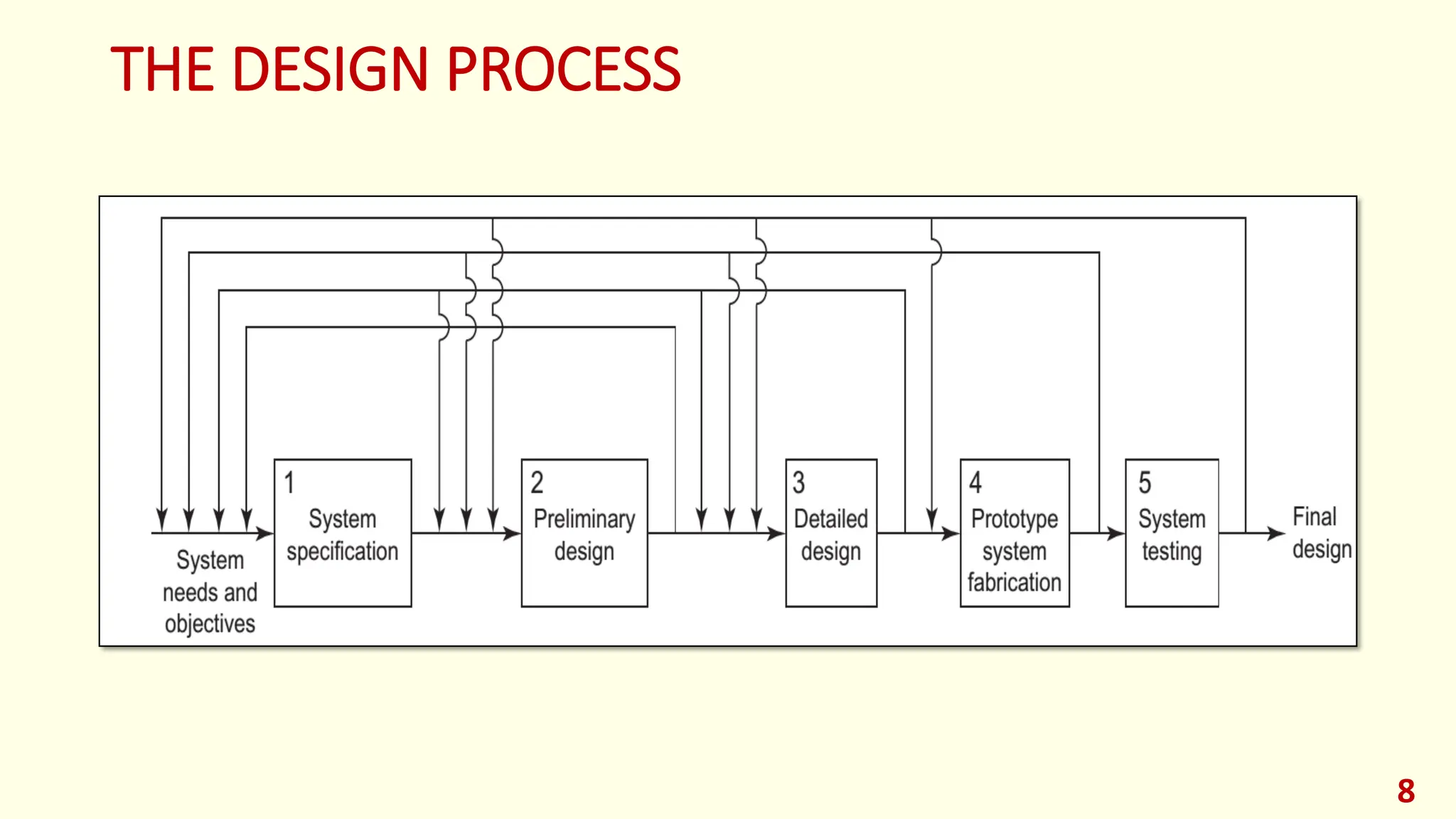
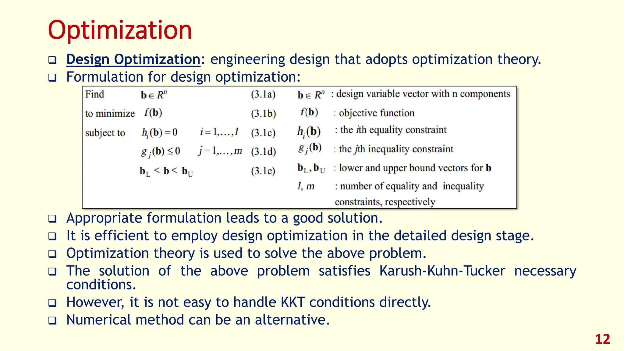
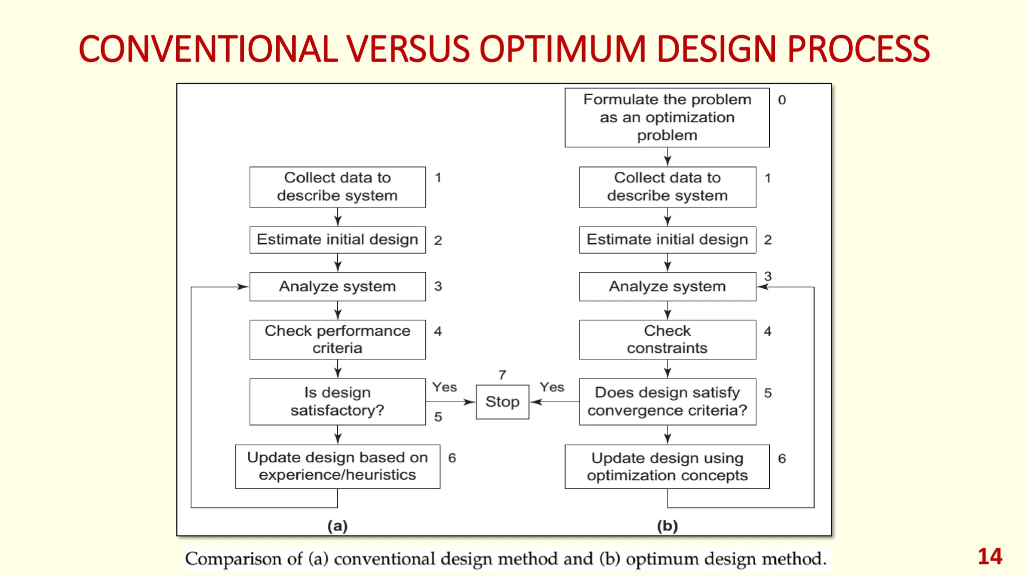
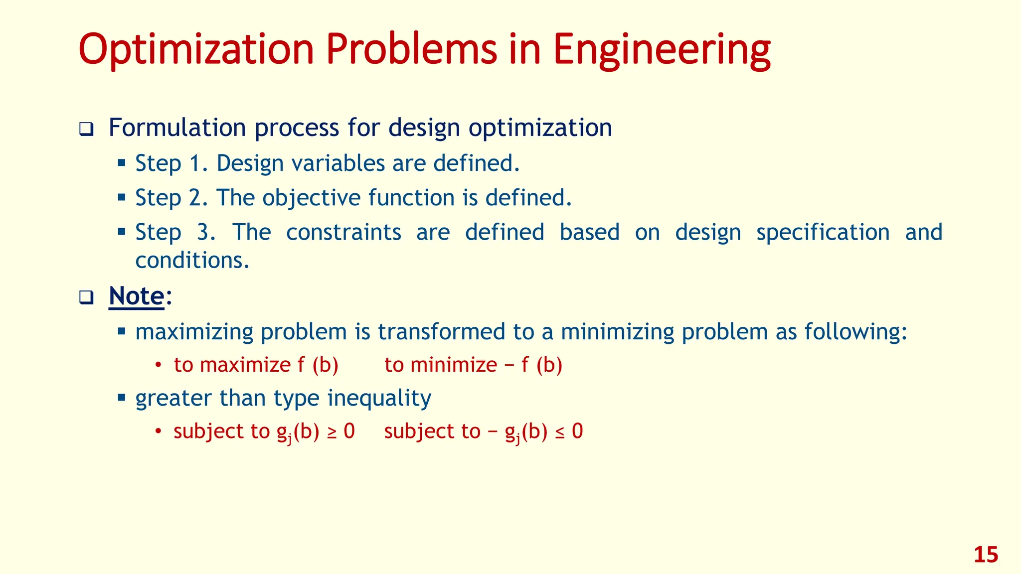
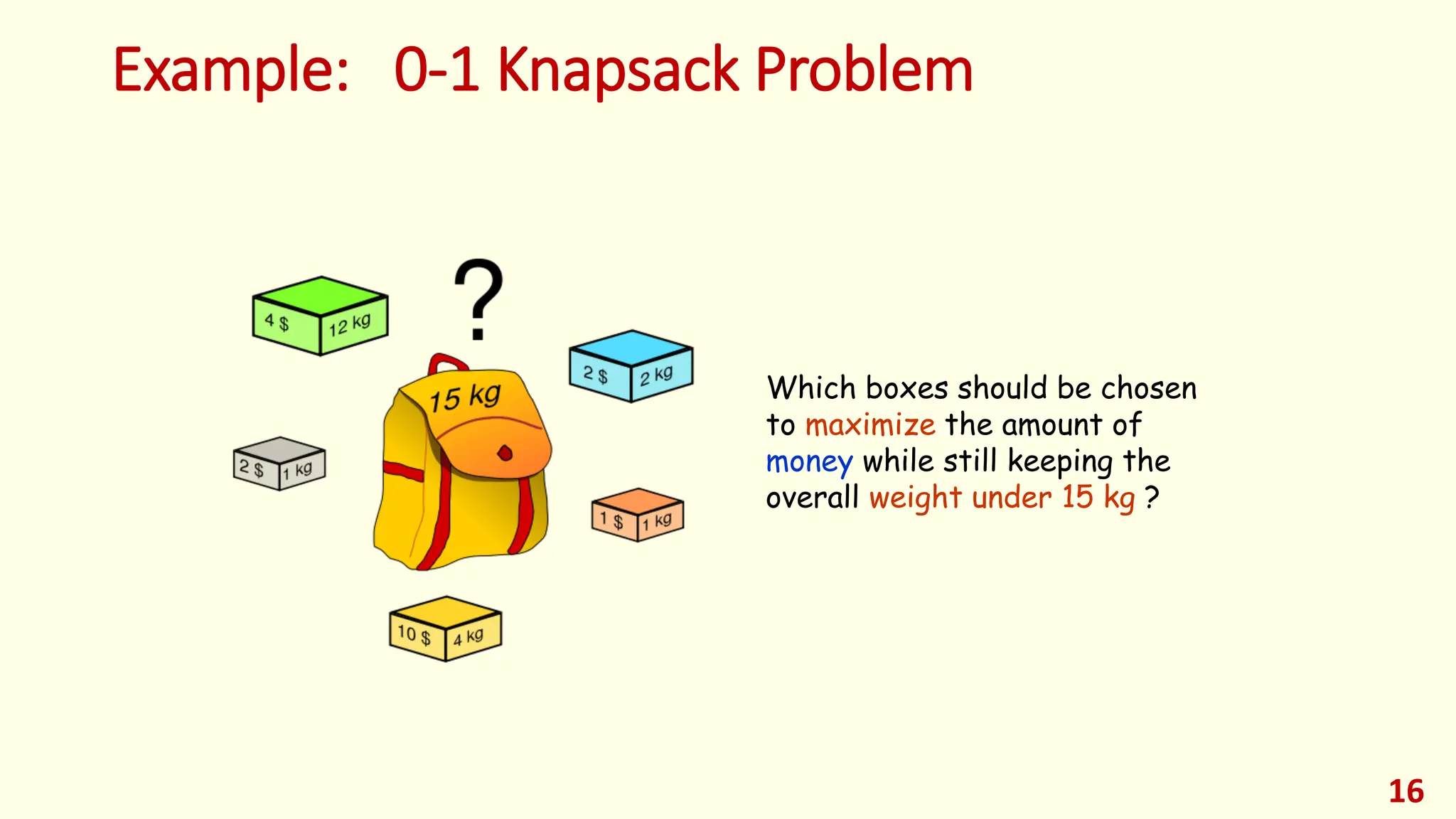
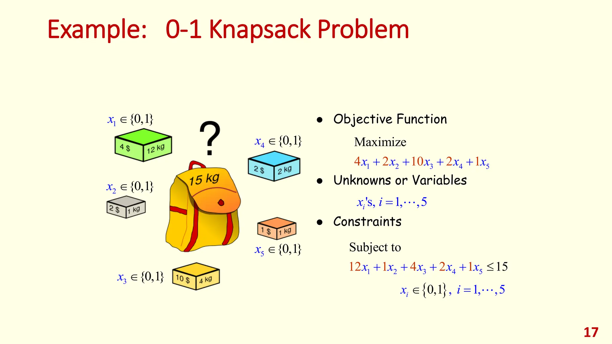
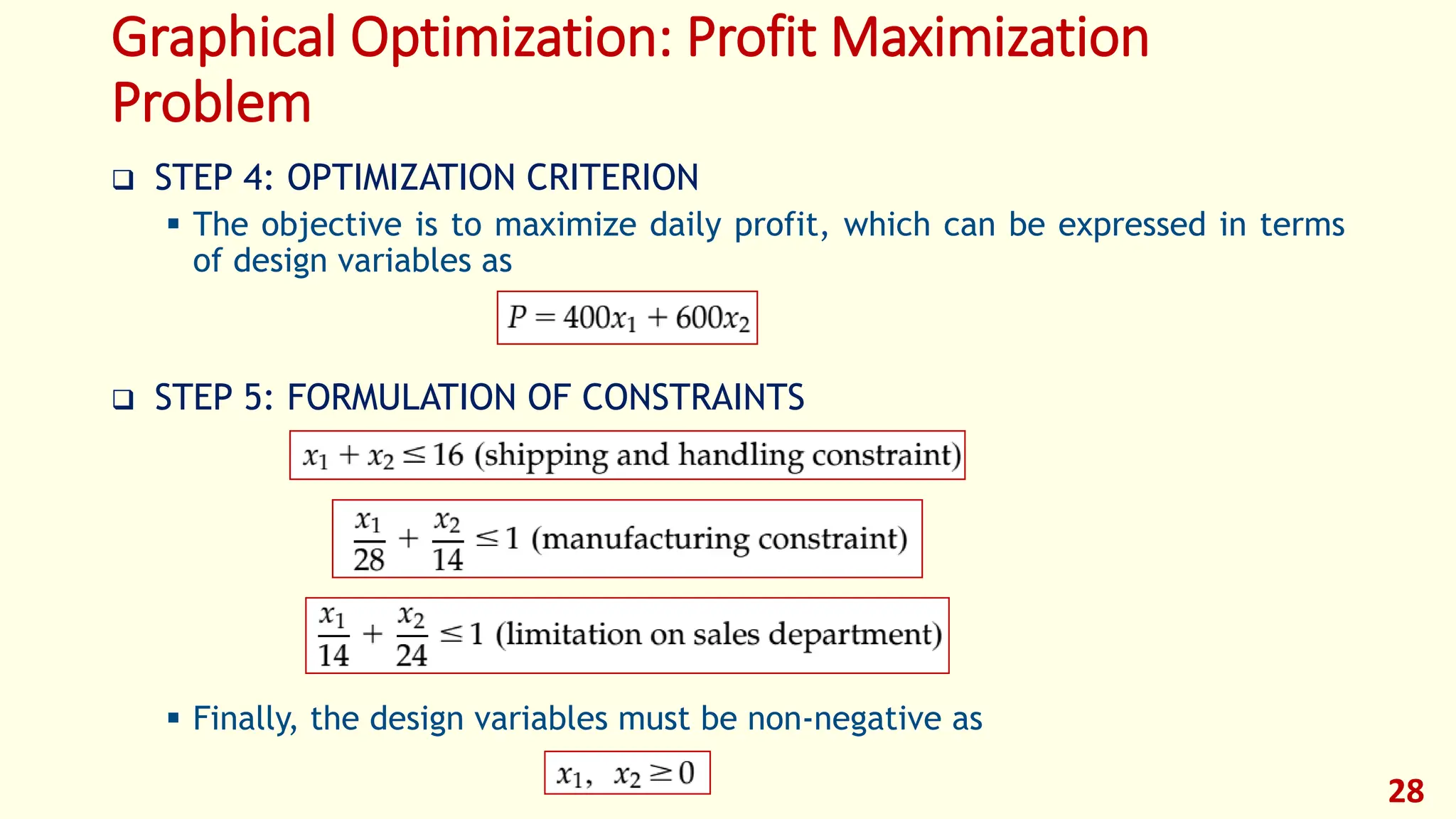
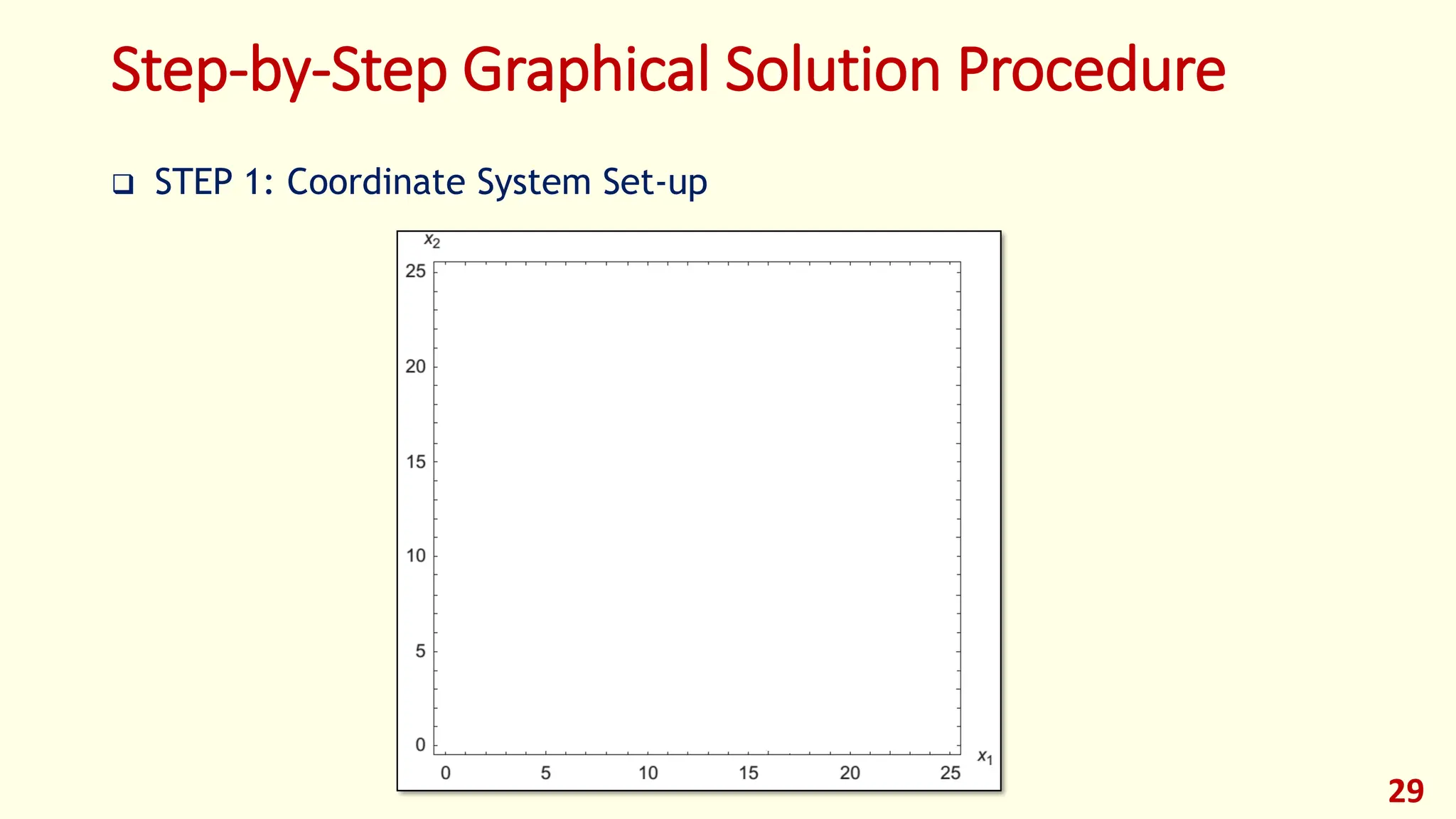
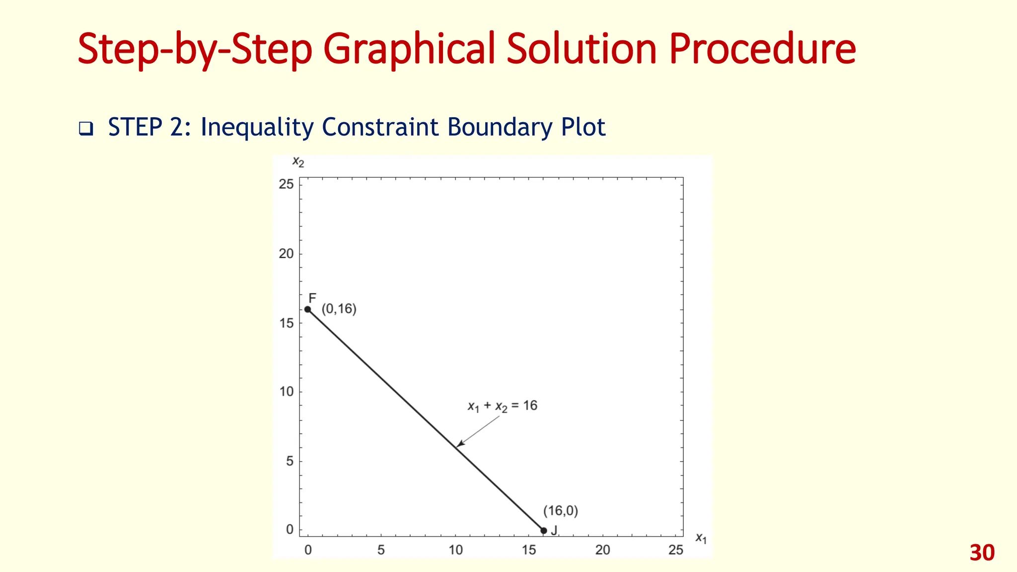
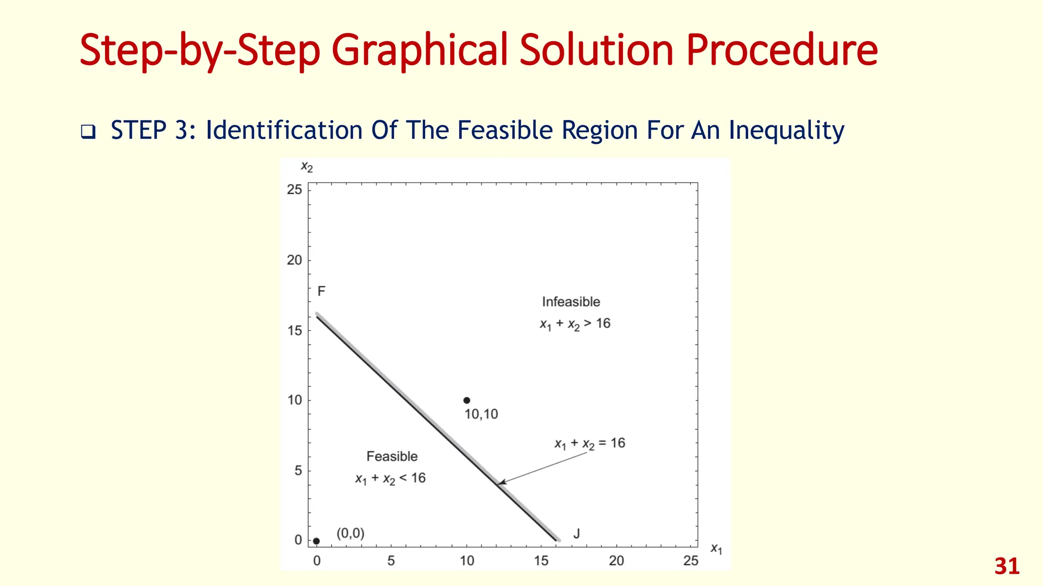
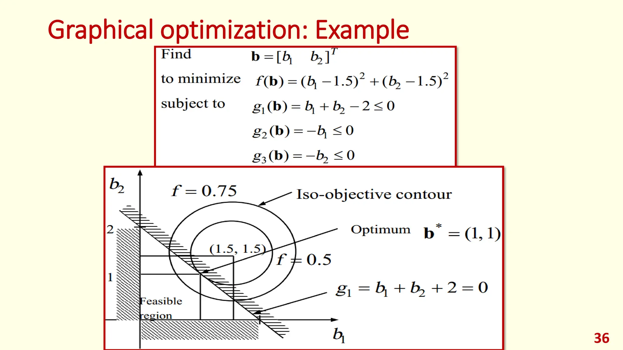
1. ‫َر‬‫د‬‫ـ‬ْ‫ق‬‫ـ‬ِ‫ن‬
،،،
‫لما‬
‫اننا‬ ‫نصدق‬
ْ
ْ‫ق‬ِ‫ن‬
‫َر‬‫د‬
LECTURE (1)
Introduction To Optimum Design
Assoc. Prof. Amr E. Mohamed
Faculty of Engineering - Helwan University

2. Reference Books
❑ Textbook: J.S. Arora “Introduction to OptimumDesign, Third Edition”,
Elsevier.
❑ Grading:
▪ Assignments + Midterms + Project (40%),
▪ Final (60%).
❑ Assignments: Assignment is due at the begging of the class. Late
Assignment is not accepted.
2

3. Objective
❑ Understand optimization approaches to engineering design.
❑ Study the numerical optimization techniques for engineering design.
❑ Studying Evolutionary algorithms which are relatively new, but very
powerful techniques used to find solutions to many real-world search
and optimization problems.
❑ Practice the systematic process on a semester-long project.
3

4. Outlines
❑ Formulation of optimization problems
❑ Optimization concepts using the graphical method
❑ Optimality conditions for unconstrained and constrained problems
❑ Use of Excel and MATLAB illustrating optimum design of practical
problems
❑ Linear programming
❑ Numerical methods for unconstrained and constrained problems
❑ Theory and numerical methods for unconstrained optimization
❑ Theory and numerical methods for constrained optimization
❑ Midterm Exam
4

5. Outlines (cont.’)
❑ Linear and quadratic programming
❑ Duality theory in nonlinear programming
❑ Rate of convergence of iterative algorithms
❑ Derivation of numerical methods
❑ Derivation of direct search methods
❑ Methods for discrete variable problems
❑ Nature-inspired search methods
❑ Multi-objective optimization
❑ Final exam/Project presentation
5

6. Introduction to Design Optimization
6

7. Introduction to Design Optimization
❑ Engineering consists of a number of well-established activities,
including analysis, design, fabrication, sales, research, and
development of systems.
❑ The design of a system can be formulated as problems of optimization
in which a performance measure is optimized while all other
requirements are satisfied.
❑ Many numerical methods of optimization have been developed and used
to design better systems.
❑ Design process, rather than optimization theory, is emphasized.
❑ Any problem in which certain parameters need to be determined to
satisfy constraints can be formulated as one optimization problem.
7

8. THE DESIGN PROCESS
8

9. ENGINEERING DESIGN Vs ENGINEERING ANALYSIS
❑ Engineering analysis
▪ It is concerned with determining the behavior of an existing system or a trial
system being designed for a given task.
▪ Determination of the behavior of the system implies calculation of its
response to specified inputs.
❑ Engineering design activities
▪ It calculates the sizes and shapes of various parts of the system to meet
performance requirements.
▪ The design of a system is an iterative process;
• we estimate a design and analyze it to see if it performs according to given
specifications. If it does, we have anacceptable (feasible) design, although we
may still want to change it to improve its performance.
9

10. Introduction to optimization Problem
❑ Optimization is an essential part of design activity in all major disciplines.
❑ It is process of search that seek to optimize (either maximization of benefits or
minimize of cost) a mathematical function of several variables (design
variables) subjected to certain constraints (equality or inequality).
❑ The subject of optimization is quite general in the sense that
▪ It can be looked in different ways depending on the approach (algebraic or
geometric)
▪ The natural of variables may be real (continuous), integer (discrete) or mix of both.
10

11. Introduction to optimization Problem (Cont.)
❑ Further, the optimization problem can be classified into two groups
▪ Static Optimization Problems: it is concerned with design variables (that involved
in the objective function) that are not changing w.r.t time. Techniques are used to
solve this problem are
• Ordinary calculus.
• Lagrange multiplier
• Linear or Nonlinear programming.
▪ Dynamic Optimization Problems: it is concerned with variables that are changing
w.r.t. time, and the time is involved in the problem statement. Techniques are used
to solve this problem are
• Calculus of variations
• Dynamic programming.
• Convex optimization.
11

12. Optimization
❑ Design Optimization: engineering design that adopts optimization theory.
❑ Formulation for design optimization:
❑ Appropriate formulation leads to a good solution.
❑ It is efficient to employ design optimization in the detailed design stage.
❑ Optimization theory is used to solve the above problem.
❑ The solution of the above problem satisfies Karush-Kuhn-Tucker necessary
conditions.
❑ However, it is not easy to handle KKT conditions directly.
❑ Numerical method can be an alternative.
12

13. What is Optimization?
❑ Objective Function
▪ A function to be minimized or maximized
❑ Unknowns or Variables
▪ Affect the value of the objective function
❑ Constraints
▪ Restrict unknowns to take on certain values but exclude others
13

14. CONVENTIONAL VERSUS OPTIMUM DESIGN PROCESS
14

15. Optimization Problems in Engineering
❑ Formulation process for design optimization
▪ Step 1. Design variables are defined.
▪ Step 2. The objective function is defined.
▪ Step 3. The constraints are defined based on design specification and
conditions.
❑ Note:
▪ maximizing problem is transformed to a minimizing problem as following:
• to maximize f (b) to minimize − f (b)
▪ greater than type inequality
• subject to gj(b) ≥ 0 subject to − gj(b) ≤ 0
15

16. Example: 0-1 Knapsack Problem
16
Which boxes should be chosen
to maximize the amount of
money while still keeping the
overall weight under 15 kg ?

17. Example: 0-1 Knapsack Problem
17
1 {0,1}
x 
2 {0,1}
x 
3 {0,1}
x 
5 {0,1}
x 
4 {0,1}
x 
⚫ Objective Function
⚫ Unknowns or Variables
⚫ Constraints
's, 1, ,5
i
x i =
 , ,
0,1 1, 5
i
x i
 =
1 2 3 4 5
4 2 10 2 1
Maximize
x x x x x
+ + + +
1 2 3 4 5
12 1
Subject t
15
4 2
o
1
x x x x x
+ + 
+ +

18. 1 2 3 4 5
4 2 10 2
Maxim 1
ize x x x x x
+ + + +
 
1 2 3 4 5
12 1 4 2
Subject to 15,
0,1 , 1, ,5
1
i
x x x x x
x i
+ + + + 
 =
Example: 0-1 Knapsack Problem

19. Example: Design a “Can’
19

20. Example: Design a “Can’
❑ Side constraints are necessary part of the solution techniques
❑ Side constraints determine the acceptable region of the solution.
❑ Graphical representation:
20
x1
x2
22
5
3 5

21. Example: Design a “Can’
❑ Our example is
❑ Static optimization problem
❑ Nonlinear optimization problem
21

22. Classification of optimization problems
Classification based on:
1. Constraints
• Unconstrained optimization problem
• Constrained optimization problem
2. Nature of the design variables
• Static optimization problems
• Dynamic optimization problems
22

23. Classification of optimization problems
Classification based on:
3. Physical structure of the problem
• Optimal control problems
• Non-optimal control problems
4. Nature of the equations involved
• Linear programming problem
• Nonlinear programming problem
• Quadratic programming problem
• Geometric programming problem
23

24. Classification of optimization problems
Classification based on:
5. Permissable values of the design variables
• Integer programming problems
• Real valued programming problems
6. Deterministic nature of the variables
• Deterministic programming problem
• Stochastic programming problem
24

25. Classification of optimization problems
Classification based on:
7. Separability of the functions
• Separable programming problems
• Non-separable programming problems
8. Number of the objective functions
• Single objective programming problem
• Multiobjective programming problem
25

26. Graphical Optimization
❑ Finds an optimum solution by drawing the objective and constraint
functions on a plane.
❑ Not useful in practical design problem
26

27. Graphical Optimization: Profit Maximization Problem
❑ STEP 1: PROJECT/PROBLEM DESCRIPTION
▪ A company manufactures two machines, A and B. Using available resources,
either 28 A or 14 B can be manufactured daily. The sales department can sell
up to 14 A-machines or 24 B-machines. The shipping facility can handle no
more than 16 machines per day. The company makes a profit of $400 on
each A-machine and $600 on each B-machine. How many A and B machines
should the company manufacture every day to maximize its profit?
❑ STEP 2: DATA AND INFORMATION COLLECTION
▪ Data and information are defined in the project statement.
❑ STEP 3: DEFINITION OF DESIGN VARIABLES
▪ The following two design variables are identified in the problem statement:
• x1 = number of A-machines manufactured each day
• x2 = number of B-machines manufactured each day
27

28. Graphical Optimization: Profit Maximization
Problem
❑ STEP 4: OPTIMIZATION CRITERION
▪ The objective is to maximize daily profit, which can be expressed in terms
of design variables as
❑ STEP 5: FORMULATION OF CONSTRAINTS
▪ Finally, the design variables must be non-negative as
28

29. Step-by-Step Graphical Solution Procedure
❑ STEP 1: Coordinate System Set-up
29

30. Step-by-Step Graphical Solution Procedure
❑ STEP 2: Inequality Constraint Boundary Plot
30

31. Step-by-Step Graphical Solution Procedure
❑ STEP 3: Identification Of The Feasible Region For An Inequality
31

32. Step-by-Step Graphical Solution Procedure
❑ STEP 4: Identification Of The Feasible Region
32

33. Step-by-Step Graphical Solution Procedure
❑ STEP 5: Plotting Of Objective Function Contours
33
To plot a contour through the feasible
region, we need to assign it a value. To
obtain this value, consider a point in the
feasible region and evaluate the profit
function there. For example, at point
(6,4), P is P=6x400+4x600=4800. To plot
the P=4800 contour, we plot the function
400x1+600x2=4800. This contour is a
straight line.

34. Step-by-Step Graphical Solution Procedure
❑ Step 6: Identification Of The Optimum Solution
34

35. MATLAB Solution
❑ profit_max.m
35

36. Graphical optimization: Example
36

37. 37