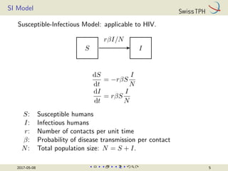
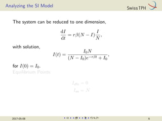
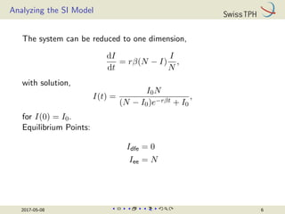
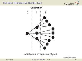
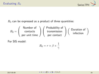
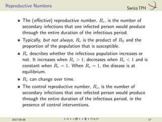
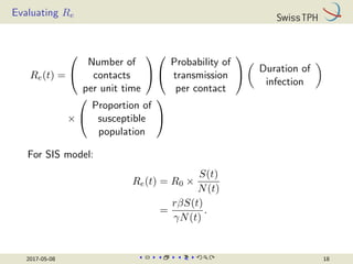
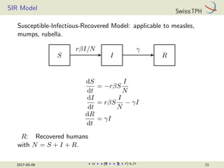
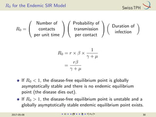
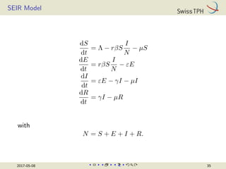
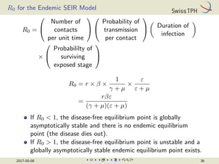
This document provides an introduction to SEIR models for infectious diseases. It outlines the SI, SIS, and SIR models and defines key concepts like the basic reproductive number R0. R0 is defined as the number of secondary infections produced by one infected individual in a fully susceptible population. The document explains that the disease-free equilibrium is stable if R0 < 1 and unstable if R0 > 1. It also introduces the effective reproductive number Re and control reproductive number Rc.

1. Introduction to SEIR Models
Nakul Chitnis
Workshop on Mathematical Models of Climate Variability,
Environmental Change and Infectious Diseases
Trieste, Italy
8 May 2017
Department of Epidemiology and Public Health
Health Systems Research and
Dynamical Modelling Unit

2. Outline
SI Model
SIS Model
The Basic Reproductive Number (R0)
SIR Model
SEIR Model
2017-05-08 2

3. Mathematical Models of Infectious Diseases
Population-based models
I Can be deterministic or stochastic
I Continuous time
• Ordinary differential equations
• Partial differential equations
• Delay differential equations
• Integro-differential equations
I Discrete time
• Difference equations
Agent-based/individual-based models
I Usually stochastic
I Usually discrete time
2017-05-08 3

4. Mathematical Models of Infectious Diseases
Population-based models
I Can be deterministic or stochastic
I Continuous time
• Ordinary differential equations
• Partial differential equations
• Delay differential equations
• Integro-differential equations
I Discrete time
• Difference equations
Agent-based/individual-based models
I Usually stochastic
I Usually discrete time
2017-05-08 3

5. Outline
SI Model
SIS Model
The Basic Reproductive Number (R0)
SIR Model
SEIR Model
2017-05-08 4

6. SI Model
Susceptible-Infectious Model: applicable to HIV.
S I
rβI/N
dS
dt
= −rβS
I
N
dI
dt
= rβS
I
N
S: Susceptible humans
I: Infectious humans
r: Number of contacts per unit time
β: Probability of disease transmission per contact
N: Total population size: N = S + I.
2017-05-08 5

7. Analyzing the SI Model
The system can be reduced to one dimension,
dI
dt
= rβ(N − I)
I
N
,
with solution,
I(t) =
I0N
(N − I0)e−rβt + I0
,
for I(0) = I0.
Equilibrium Points:
Idfe = 0
Iee = N
2017-05-08 6

8. Analyzing the SI Model
The system can be reduced to one dimension,
dI
dt
= rβ(N − I)
I
N
,
with solution,
I(t) =
I0N
(N − I0)e−rβt + I0
,
for I(0) = I0.
Equilibrium Points:
Idfe = 0
Iee = N
2017-05-08 6

9. Numerical Solution of SI Model
0 5 10 15 20
0
200
400
600
800
1000
Time (Years)
Infectious
Humans
With r = 365/3 years−1, β = 0.005, N = 1000, and I(0) = 1.
2017-05-08 7

10. Definition of Transmission Parameters
Note that in some models, usually of diseases where contacts
are not well defined, rβ (the number of contacts per unit time
multiplied by the probability of disease transmission per
contact) are combined into one parameter (often also called β
— the number of adequate contacts per unit time).
For diseases where a contact is well defined (such as sexually
transmitted diseases like HIV or vector-borne diseases like
malaria), it is usually more appropriate to separate the contact
rate, r, and the probability of transmission per contact, β.
For diseases where contacts are not well defined (such as
air-borne diseases like influenza) it is usually more appropriate
to combine the two into one parameter.
2017-05-08 8

11. Outline
SI Model
SIS Model
The Basic Reproductive Number (R0)
SIR Model
SEIR Model
2017-05-08 9

12. SIS Model
Susceptible-Infectious-Susceptible Model: applicable to the
common cold.
S I
rβI/N
γ
dS
dt
= −rβS
I
N
+ γI
dI
dt
= rβS
I
N
− γI
γ: Per-capita recovery rate
2017-05-08 10

13. Analyzing the SIS Model
The system can be reduced to one dimension,
dI
dt
= rβ(N − I)
I
N
− γI,
with solution,
I(t) =
N
rβ · (rβ − γ)
1 +
N
rβ
(rβ−γ)
I0
− 1
e−(rβ−γ)t
,
for I(0) = I0.
Equilibrium Points:
Idfe = 0
Iee =
(rβ − γ)N
rβ
2017-05-08 11

14. Analyzing the SIS Model
The system can be reduced to one dimension,
dI
dt
= rβ(N − I)
I
N
− γI,
with solution,
I(t) =
N
rβ · (rβ − γ)
1 +
N
rβ
(rβ−γ)
I0
− 1
e−(rβ−γ)t
,
for I(0) = I0.
Equilibrium Points:
Idfe = 0
Iee =
(rβ − γ)N
rβ
2017-05-08 11

15. Numerical Solution of SIS Model
0 10 20 30 40 50
0
200
400
600
800
1000
Time (Days)
Infectious
Humans
With rβ = 0.5 days−1, γ = 0.1 days−1, N = 1000, and I(0) = 1.
2017-05-08 12

16. Outline
SI Model
SIS Model
The Basic Reproductive Number (R0)
SIR Model
SEIR Model
2017-05-08 13

17. The Basic Reproductive Number (R0)
of uncertainty that may be prioritized for urgent res
Disease is ende
Initial phase of epidemic (R0 = 3)
Generation
0 1 2
Pan-InfORM (2009)
2017-05-08 14

18. Definition of R0
The basic reproductive number, R0, is the number of
secondary infections that one infected person would produce
in a fully susceptible population through the entire duration of
the infectious period.
R0 provides a threshold condition for the stability of the
disease-free equilibrium point (for most models):
I The disease-free equilibrium point is locally asymptotically
stable when R0 1: the disease dies out.
I The disease-free equilibrium point is unstable when R0 1:
the disease establishes itself in the population or an epidemic
occurs.
I For a given model, R0 is fixed over all time.
This definition is only valid for simple homogeneous
autonomous models.
Can define similar threshold conditions for more complicated
models that include heterogeneity and/or seasonality but the
basic definition no longer holds.
2017-05-08 15

19. Definition of R0
The basic reproductive number, R0, is the number of
secondary infections that one infected person would produce
in a fully susceptible population through the entire duration of
the infectious period.
R0 provides a threshold condition for the stability of the
disease-free equilibrium point (for most models):
I The disease-free equilibrium point is locally asymptotically
stable when R0 1: the disease dies out.
I The disease-free equilibrium point is unstable when R0 1:
the disease establishes itself in the population or an epidemic
occurs.
I For a given model, R0 is fixed over all time.
This definition is only valid for simple homogeneous
autonomous models.
Can define similar threshold conditions for more complicated
models that include heterogeneity and/or seasonality but the
basic definition no longer holds.
2017-05-08 15

20. Definition of R0
The basic reproductive number, R0, is the number of
secondary infections that one infected person would produce
in a fully susceptible population through the entire duration of
the infectious period.
R0 provides a threshold condition for the stability of the
disease-free equilibrium point (for most models):
I The disease-free equilibrium point is locally asymptotically
stable when R0 1: the disease dies out.
I The disease-free equilibrium point is unstable when R0 1:
the disease establishes itself in the population or an epidemic
occurs.
I For a given model, R0 is fixed over all time.
This definition is only valid for simple homogeneous
autonomous models.
Can define similar threshold conditions for more complicated
models that include heterogeneity and/or seasonality but the
basic definition no longer holds.
2017-05-08 15

21. Definition of R0
The basic reproductive number, R0, is the number of
secondary infections that one infected person would produce
in a fully susceptible population through the entire duration of
the infectious period.
R0 provides a threshold condition for the stability of the
disease-free equilibrium point (for most models):
I The disease-free equilibrium point is locally asymptotically
stable when R0 1: the disease dies out.
I The disease-free equilibrium point is unstable when R0 1:
the disease establishes itself in the population or an epidemic
occurs.
I For a given model, R0 is fixed over all time.
This definition is only valid for simple homogeneous
autonomous models.
Can define similar threshold conditions for more complicated
models that include heterogeneity and/or seasonality but the
basic definition no longer holds.
2017-05-08 15

22. Evaluating R0
R0 can be expressed as a product of three quantities:
R0 =


Number of
contacts
per unit time




Probability of
transmission
per contact


Duration of
infection
For SIS model:
R0 = r × β ×
1
γ
2017-05-08 16

23. Reproductive Numbers
The (effective) reproductive number, Re, is the number of
secondary infections that one infected person would produce
through the entire duration of the infectious period.
Typically, but not always, Re is the product of R0 and the
proportion of the population that is susceptible.
Re describes whether the infectious population increases or
not. It increases when Re 1; decreases when Re 1 and is
constant when Re = 1. When Re = 1, the disease is at
equilibrium.
Re can change over time.
The control reproductive number, Rc, is the number of
secondary infections that one infected person would produce
through the entire duration of the infectious period, in the
presence of control interventions.
2017-05-08 17

24. Reproductive Numbers
The (effective) reproductive number, Re, is the number of
secondary infections that one infected person would produce
through the entire duration of the infectious period.
Typically, but not always, Re is the product of R0 and the
proportion of the population that is susceptible.
Re describes whether the infectious population increases or
not. It increases when Re 1; decreases when Re 1 and is
constant when Re = 1. When Re = 1, the disease is at
equilibrium.
Re can change over time.
The control reproductive number, Rc, is the number of
secondary infections that one infected person would produce
through the entire duration of the infectious period, in the
presence of control interventions.
2017-05-08 17

25. Reproductive Numbers
The (effective) reproductive number, Re, is the number of
secondary infections that one infected person would produce
through the entire duration of the infectious period.
Typically, but not always, Re is the product of R0 and the
proportion of the population that is susceptible.
Re describes whether the infectious population increases or
not. It increases when Re 1; decreases when Re 1 and is
constant when Re = 1. When Re = 1, the disease is at
equilibrium.
Re can change over time.
The control reproductive number, Rc, is the number of
secondary infections that one infected person would produce
through the entire duration of the infectious period, in the
presence of control interventions.
2017-05-08 17

26. Reproductive Numbers
The (effective) reproductive number, Re, is the number of
secondary infections that one infected person would produce
through the entire duration of the infectious period.
Typically, but not always, Re is the product of R0 and the
proportion of the population that is susceptible.
Re describes whether the infectious population increases or
not. It increases when Re 1; decreases when Re 1 and is
constant when Re = 1. When Re = 1, the disease is at
equilibrium.
Re can change over time.
The control reproductive number, Rc, is the number of
secondary infections that one infected person would produce
through the entire duration of the infectious period, in the
presence of control interventions.
2017-05-08 17

27. Reproductive Numbers
The (effective) reproductive number, Re, is the number of
secondary infections that one infected person would produce
through the entire duration of the infectious period.
Typically, but not always, Re is the product of R0 and the
proportion of the population that is susceptible.
Re describes whether the infectious population increases or
not. It increases when Re 1; decreases when Re 1 and is
constant when Re = 1. When Re = 1, the disease is at
equilibrium.
Re can change over time.
The control reproductive number, Rc, is the number of
secondary infections that one infected person would produce
through the entire duration of the infectious period, in the
presence of control interventions.
2017-05-08 17

28. Evaluating Re
Re(t) =


Number of
contacts
per unit time




Probability of
transmission
per contact


Duration of
infection
×


Proportion of
susceptible
population


For SIS model:
Re(t) = R0 ×
S(t)
N(t)
=
rβS(t)
γN(t)
.
2017-05-08 18

29. The Basic Reproductive Number (R0)
http://www.cameroonweb.com/CameroonHomePage/NewsArchive/Ebola-How-does-it-compare-316932
2017-05-08 19

30. Outline
SI Model
SIS Model
The Basic Reproductive Number (R0)
SIR Model
SEIR Model
2017-05-08 20

31. SIR Model
Susceptible-Infectious-Recovered Model: applicable to measles,
mumps, rubella.
S I R
rβI/N γ
dS
dt
= −rβS
I
N
dI
dt
= rβS
I
N
− γI
dR
dt
= γI
R: Recovered humans
with N = S + I + R.
2017-05-08 21

32. Analyzing the SIR Model
Can reduce to two dimensions by ignoring the equation for R
and using R = N − S − I.
Can no longer analytically solve these equations.
Infinite number of equilibrium points with I∗ = 0.
Perform phase portrait analysis.
Estimate final epidemic size.
2017-05-08 22

33. R0 for the SIR Model
R0 =


Number of
contacts
per unit time




Probability of
transmission
per contact


Duration of
infection
R0 = r × β ×
1
γ
=
rβ
γ
If R0 1, introduced cases do not lead to an epidemic (the
number of infectious individuals decreases towards 0).
If R0 1, introduced cases can lead to an epidemic
(temporary increase in the number of infectious individuals).
Re(t) =
rβ
γ
S(t)
N
2017-05-08 23

34. Phase Portrait of SIR Model
THE MATHEMATICS OF INFECTIOUS DISEASES 605
0 0.2 0.4 0.6 0.8 1
susceptible fraction, s
0
0.2
0.4
0.6
0.8
1
infective
fraction,
i
smax
↑
= 1
σ
σ = 3
Fig. 2 Phase plane portrait for the classic SIR epidemic model with contact number σ = 3.
Hethcote (2000)
2017-05-08 24

35. Numerical Solution of SIR Model
0 20 40 60 80 100
0
200
400
600
800
1000
Time (Days)
Humans
Susceptible
Infectious
Recovered
With rβ = 0.3 days−1, γ = 0.1 days−1, N = 1000, and
S(0) = 999, I(0) = 1 and R(0) = 0.
2017-05-08 25

36. Numerical Solution of SIR Model
0 20 40 60 80 100
0
200
400
600
800
1000
Time (Days)
Humans
Susceptible
Infectious
Recovered
With rβ = 0.3 days−1, γ = 0.1 days−1, N = 1000, and
S(0) = 580, I(0) = 20 and R(0) = 400.
2017-05-08 26

37. Human Demography
Need to include human demographics for diseases where the
time frame of the disease dynamics is comparable to that of
human demographics.
There are many different ways of modeling human
demographics
I Constant immigration rate
I Constant per-capita birth and death rates
I Density-dependent death rate
I Disease-induced death rate.
2017-05-08 27

38. Endemic SIR Model
S I R
rβI/N γ
Birth
Death Death Death
Λ
µ µ µ
dS
dt
= Λ − rβS
I
N
− µS
dI
dt
= rβS
I
N
− γI − µI
dR
dt
= γI − µR
N = S + I + R
Λ: Constant recruitment rate
µ: Per-capita removal rate
2017-05-08 28

39. Analyzing the Endemic SIR Model
Can no longer reduce the dimension or solve analytically.
There are two equilibrium points: disease-free and endemic
Sdfe =
Λ
µ
See =
Λ(γ + µ)
rβµ
Idfe = 0 Iee =
Λ(rβ − (γ + µ))
rβ(γ + µ)
Rdfe = 0 Ree =
γΛ(rβ − (γ + µ))
rβµ(γ + µ)
Can perform stability analysis of these equilibrium points and
draw phase portraits.
2017-05-08 29

40. R0 for the Endemic SIR Model
R0 =


Number of
contacts
per unit time




Probability of
transmission
per contact


Duration of
infection
R0 = r × β ×
1
γ + µ
=
rβ
γ + µ
If R0 1, the disease-free equilibrium point is globally
asymptotically stable and there is no endemic equilibrium
point (the disease dies out).
If R0 1, the disease-free equilibrium point is unstable and a
globally asymptotically stable endemic equilibrium point exists.
2017-05-08 30

41. Numerical Solution of Endemic SIR Model
0 20 40 60 80 100
0
200
400
600
800
1000
Time (Days)
Humans
Susceptible
Infectious
Recovered
With rβ = 0.3 days−1, γ = 0.1 days−1, µ = 1/60 years−1,
Λ = 1000/60 years−1, and S(0) = 999, I(0) = 1 and R(0) = 0.
2017-05-08 31

42. Numerical Solution of Endemic SIR Model
0 20 40 60 80 100 120
0
200
400
600
800
1000
Time (Years)
Humans
Susceptible
Infectious
Recovered
With rβ = 0.3 days−1, γ = 0.1 days−1, µ = 1/60 years−1,
Λ = 1000/60 years−1, and S(0) = 999, I(0) = 1 and R(0) = 0.
2017-05-08 32

43. Outline
SI Model
SIS Model
The Basic Reproductive Number (R0)
SIR Model
SEIR Model
2017-05-08 33

44. SEIR Model
Susceptible-Exposed-Infectious-Recovered Model: applicable to
measles, mumps, rubella.
S E I R
rβI/N ε γ
Birth
Death Death Death Death
Λ
µ µ µ µ
E: Exposed (latent) humans
ε: Per-capita rate of progression to infectious state
2017-05-08 34

45. SEIR Model
dS
dt
= Λ − rβS
I
N
− µS
dE
dt
= rβS
I
N
− εE
dI
dt
= εE − γI − µI
dR
dt
= γI − µR
with
N = S + E + I + R.
2017-05-08 35

46. R0 for the Endemic SEIR Model
R0 =


Number of
contacts
per unit time




Probability of
transmission
per contact


Duration of
infection
×


Probabililty of
surviving
exposed stage


R0 = r × β ×
1
γ + µ
×
ε
ε + µ
=
rβε
(γ + µ)(ε + µ)
If R0 1, the disease-free equilibrium point is globally
asymptotically stable and there is no endemic equilibrium
point (the disease dies out).
If R0 1, the disease-free equilibrium point is unstable and a
globally asymptotically stable endemic equilibrium point exists.
2017-05-08 36

47. Extensions to Compartmental Models
Basic compartmental models assume a homogeneous
population.
Divide the population into different groups based on infection
status:
M: Humans with maternal immunity
S: Susceptible humans
E: Exposed (infected but not yet infectious) humans
I: Infectious humans
R: Recovered humans.
Can include time-dependent parameters to include the effects
of seasonality.
Can include additional compartments to model vaccinated and
asymptomatic individuals, and different stages of disease
progression.
Can include multiple groups to model heterogeneity, age,
spatial structure or host species.
2017-05-08 37

48. References
O. Diekmann, H. Heesterbeek, and T. Britton, Mathematical Tools for
Understanding Infectious Disease Dynamics.
Princeton Series in Theoretical and Computational Biology. Princeton University
Press, Princeton, (2013).
H. W. Hethcote, “The mathematics of infectious diseases”, SIAM Review 42,
599–653 (2000).
M. J. Keeling and P. Rohani, Modeling Infectious Diseases in Humans and
Animals.
Princeton University Press, Princeton, (2007).
2017-05-08 38