1. Chemical kinetics deals with the rates of chemical reactions rather than their thermodynamic favorability. A reaction may be energetically favorable but still proceed slowly if there is no low-energy reaction pathway.
2. The rate of a reaction is expressed as the change in concentration of a species with time. Rate laws relate the rates of reactions to concentrations of reactants and can be determined experimentally.
3. Common rate laws include zero-order, first-order, and second-order reactions. The overall order of a reaction is the sum of the exponents on the concentrations of reactants in the rate law. Kinetics aims to determine the rate laws and rate constants for reactions.


![5.8 Linear Free Energy Relationships 185
5.9 The Compensation EVect 189
5.10 Some Correlations of Rates with Solubility Parameter 191
References for Further Reading 198
Problems 199
6 Enzyme Catalysis 205
6.1 Enzyme Action 205
6.2 Kinetics of Reactions Catalyzed by Enzymes 208
6.2.1 Michaelis–Menten Analysis 208
6.2.2 Lineweaver–Burk and Eadie Analyses 213
6.3 Inhibition of Enzyme Action 215
6.3.1 Competitive Inhibition 216
6.3.2 Noncompetitive Inhibition 218
6.3.3 Uncompetitive Inhibition 219
6.4 The EVect of pH 220
6.5 Enzyme Activation by Metal Ions 223
6.6 Regulatory Enzymes 224
References for Further Reading 226
Problems 227
7 Kinetics of Reactions in the Solid State 229
7.1 Some General Considerations 229
7.2 Factors AVecting Reactions in Solids 234
7.3 Rate Laws for Reactions in Solids 235
7.3.1 The Parabolic Rate Law 236
7.3.2 The First-Order Rate Law 237
7.3.3 The Contracting Sphere Rate Law 238
7.3.4 The Contracting Area Rate Law 240
7.4 The Prout–Tompkins Equation 243
7.5 Rate Laws Based on Nucleation 246
7.6 Applying Rate Laws 249
7.7 Results of Some Kinetic Studies 252
7.7.1 The Deaquation-Anation of [Co(NH3)5H2O]Cl3 252
7.7.2 The Deaquation-Anation of [Cr(NH3)5H2O]Br3 255
7.7.3 The Dehydration of Trans-[Co(NH3)4Cl2]IO3 2H2O 256
7.7.4 Two Reacting Solids 259
References for Further Reading 261
Problems 262
Contents ix](https://image.slidesharecdn.com/chemicalkinetics-231126172917-d2fe5718/85/CHEMICAL-KINETICS-pdf-10-320.jpg)


![of the process must usually be determined experimentally. Chemical kin-
etics is largely an experimental science.
Chemical kinetics is intimately connected with the analysis of data. The
personal computers of today bear little resemblance to those of a couple of
decades ago. When one purchases a computer, it almost always comes with
software that allows the user to do much more than word processing.
Software packages such as Excel, Mathematica, MathCad, and many
other types are readily available. The tedious work of plotting points on
graph paper has been replaced by entering data in a spreadsheet. This is not
a book about computers. A computer is a tool, but the user needs to know
how to interpret the results and how to choose what types of analyses to
perform. It does little good to find that some mathematics program gives
the best fit to a set of data from the study of a reaction rate with an
arctangent or hyperbolic cosine function. The point is that although it is
likely that the reader may have access to data analysis techniques to process
kinetic data, the purpose of this book is to provide the background in the
principles of kinetics that will enable him or her to interpret the results. The
capability of the available software to perform numerical analysis is a
separate issue that is not addressed in this book.
1.1 RATES OF REACTIONS
The rate of a chemical reaction is expressed as a change in concentration of
some species with time. Therefore, the dimensions of the rate must be those
of concentration divided by time (moles=liter sec, moles=liter min, etc.). A
reaction that can be written as
A ! B (1:2)
has a rate that can be expressed either in terms of the disappearance of A or
the appearance of B. Because the concentration of A is decreasing as A is
consumed, the rate is expressed as d[A]=dt. Because the concentration of
B is increasing with time, the rate is expressed as þd[B]=dt. The mathemat-
ical equation relating concentrations and time is called the rate equation or
the rate law. The relationships between the concentrations of A and B with
time are represented graphically in Figure 1.1 for a first-order reaction in
which [A]o is 1.00 M and k ¼ 0:050 min1
.
If we consider a reaction that can be shown as
aA þ bB ! cC þ dD (1:3)
2 Principles of Chemical Kinetics](https://image.slidesharecdn.com/chemicalkinetics-231126172917-d2fe5718/85/CHEMICAL-KINETICS-pdf-13-320.jpg)
![the rate law will usually be represented in terms of a constant times some
function of the concentrations of A and B, and it can usually be written in
the form
Rate ¼ k[A]x
[B]y
(1:4)
where x and y are the exponents on the concentrations of A and B,
respectively. In this rate law, k is called the rate constant and the exponents
x and y are called the order of the reaction with respect to A and B,
respectively. As will be described later, the exponents x and y may or
may not be the same as the balancing coefficients a and b in Eq. (1.3).
The overall order of the reaction is the sum of the exponents x and y. Thus,
we speak of a second-order reaction, a third-order reaction, etc., when the
sum of the exponents in the rate law is 2, 3, etc., respectively. These
exponents can usually be established by studying the reaction using differ-
ent initial concentrations of A and B. When this is done, it is possible to
determine if doubling the concentration of A doubles the rate of the
reaction. If it does, then the reaction must be first-order in A, and the
value of x is 1. However, if doubling the concentration of A quadruples
the rate, it is clear that [A] must have an exponent of 2, and the reaction
is second-order in A. One very important point to remember is that there is
no necessary correlation between the balancing coefficients in the chemical
equation and the exponents in the rate law. They may be the same, but one
can not assume that they will be without studying the rate of the reaction.
If a reaction takes place in a series of steps, a study of the rate of the
reaction gives information about the slowest step of the reaction. We can
0
0 10 20 30 40 50
0.1
0.2
0.3
0.4
0.5
0.6
0.7
0.8
0.9
1.0
Time, min
M
A
B
FIGURE 1.1 Change in concentration of A and B for the reaction A ! B.
Fundamental Concepts of Kinetics 3](https://image.slidesharecdn.com/chemicalkinetics-231126172917-d2fe5718/85/CHEMICAL-KINETICS-pdf-14-320.jpg)
![see an analogy to this in the following illustration that involves the flow of
water,
3'' 1'' 5''
H2O in H2O out
If we study the rate of flow of water through this system of short pipes,
information will be obtained about the flow of water through a 1 pipe
since the 3 and 5 pipes do not normally offer as much resistance to flow as
does the 1 pipe. Therefore, in the language of chemical kinetics, the 1
pipe represents the rate-determining step.
Suppose we have a chemical reaction that can be written as
2A þ B ! Products (1:5)
and let us also suppose that the reaction takes place in steps that can be
written as
A þ B ! C (slow) (1:6)
C þ A ! Products (fast) (1:7)
The amount of C (known as an intermediate) that is present at any time limits
the rate of the overall reaction. Note that the sum of Eqs. (1.6) and (1.7)
gives the overall reaction that was shown in Eq. (1.5). Note also that the
formation of C depends on the reaction of one molecule of A and one of B.
That process will likely have a rate that depends on [A]1
and [B]1
. There-
fore, even though the balanced overall equation involves two molecules of
A, the slow step involves only one molecule of A. As a result, formation of
products follows a rate law that is of the form Rate ¼ k[A][B], and the
reaction is second-order (first-order in A and first-order in B). It should be
apparent that we can write the rate law directly from the balanced equation
only if the reaction takes place in a single step. If the reaction takes place in a
series of steps, a rate study will give information about steps up to and
including the slowest step, and the rate law will be determined by that step.
1.2 DEPENDENCE OF RATES ON
CONCENTRATION
In this section, we will examine the details of some rate laws that depend
on the concentration of reactants in some simple way. Although many
4 Principles of Chemical Kinetics](https://image.slidesharecdn.com/chemicalkinetics-231126172917-d2fe5718/85/CHEMICAL-KINETICS-pdf-15-320.jpg)
![complicated cases are well known (see Chapter 2), there are also a great
many reactions for which the dependence on concentration is first-order,
second-order, or zero-order.
1.2.1 First-Order
Suppose a reaction can be written as
A ! B (1:8)
and that the reaction follows a rate law of the form
Rate ¼ k[A]1
¼
d[A]
dt
(1:9)
This equation can be rearranged to give
d[A]
[A]
¼ k dt (1:10)
Equation (1.10) can be integrated but it should be integrated between the
limits of time ¼ 0 and time equal to t while the concentration varies from
the initial concentration [A]o at time zero to [A] at the later time. This can
be shown as
ð
[A]
[A]o
d[A]
[A]
¼ k
ð
t
0
dt (1:11)
When the integration is performed, we obtain
ln
[A]o
[A]
¼ kt or log
[A]o
[A]
¼
k
2:303
t (1:12)
If the equation involving natural logarithms is considered, it can be written
in the form
ln [A]o ln [A] ¼ kt (1:13)
or
ln [A] ¼ ln [A]o kt
y ¼ b þ mx
(1:14)
It must be remembered that [A]o, the initial concentration of A, has
some fixed value so it is a constant. Therefore, Eq. (1.14) can be put in the
Fundamental Concepts of Kinetics 5](https://image.slidesharecdn.com/chemicalkinetics-231126172917-d2fe5718/85/CHEMICAL-KINETICS-pdf-16-320.jpg)
![form of a linear equation where y ¼ ln[A], m ¼ k, and b ¼ ln [A]o. A graph
of ln[A] versus t will be linear with a slope of k. In order to test this rate
law, it is necessary to have data for the reaction which consists of the
concentration of A determined as a function of time. This suggests that in
order to determine the concentration of some species, in this case A,
simple, reliable, and rapid analytical methods are usually sought. Addition-
ally, one must measure time, which is not usually a problem unless the
reaction is a very rapid one.
It may be possible for the concentration of a reactant or product to be
determined directly within the reaction mixture, but in other cases a sample
must be removed for the analysis to be completed. The time necessary to
remove a sample from the reaction mixture is usually negligibly short
compared to the reaction time being measured. What is usually done for
a reaction carried out in solution is to set up the reaction in a vessel that is
held in a constant temperature bath so that fluctuations in temperature will
not cause changes in the rate of the reaction. Then the reaction is started,
and the concentration of the reactant (A in this case) is determined at
selected times so that a graph of ln[A] versus time can be made or the
data analyzed numerically. If a linear relationship provides the best fit to the
data, it is concluded that the reaction obeys a first-order rate law. Graphical
representation of this rate law is shown in Figure 1.2 for an initial concen-
tration of A of 1.00 M and k ¼ 0:020 min1
. In this case, the slope of the
line is k, so the kinetic data can be used to determine k graphically or by
means of linear regression using numerical methods to determine the slope
of the line.
–2.5
–2.0
–1.5
–1.0
–0.5
0.0
0 10 20 30 40 50 60 70 80 90 100
Time, min
ln
[A]
Slope = –k
FIGURE 1.2 First-order plot for A ! B with [A]o ¼ 1:00 M and k ¼ 0:020 min1
.
6 Principles of Chemical Kinetics](https://image.slidesharecdn.com/chemicalkinetics-231126172917-d2fe5718/85/CHEMICAL-KINETICS-pdf-17-320.jpg)
![The units on k in the first-order rate law are in terms of time1
. The left-
hand side of Eq. (1.12) has [concentration]=[concentration], which causes
the units to cancel. However, the right-hand side of the equation will be
dimensionally correct only if k has the units of time1
, because only then
will kt have no units.
The equation
ln [A] ¼ ln [A]o kt (1:15)
can also be written in the form
[A] ¼ [A]o ekt
(1:16)
From this equation, it can be seen that the concentration of A decreases
with time in an exponential way. Such a relationship is sometimes referred
to as an exponential decay.
Radioactive decay processes follow a first-order rate law. The rate of
decay is proportional to the amount of material present, so doubling the
amount of radioactive material doubles the measured counting rate of decay
products. When the amount of material remaining is one-half of the
original amount, the time expired is called the half-life. We can calculate
the half-life easily using Eq. (1.12). At the point where the time elapsed is
equal to one half-life, t ¼ t1=2, the concentration of A is one-half the initial
concentration or [A]o=2. Therefore, we can write
ln
[A]o
[A]
¼ ln
[A]o
[A]o
2
¼ kt1=2 ¼ ln 2 ¼ 0:693 (1:17)
The half-life is then given as
t1=2 ¼
0:693
k
(1:18)
and it will have units that depend on the units on k. For example, if k is
in hr1
, then the half-life will be given in hours, etc. Note that for a
process that follows a first-order rate law, the half-life is independent of
the initial concentration of the reactant. For example, in radioactive decay
the half-life is independent of the amount of starting nuclide. This means
that if a sample initially contains 1000 atoms of radioactive material, the
half-life is exactly the same as when there are 5000 atoms initially present.
It is easy to see that after one half-life the amount of material remaining
is one-half of the original; after two half-lives, the amount remaining is
one-fourth of the original; after three half-lives, the amount remaining
Fundamental Concepts of Kinetics 7](https://image.slidesharecdn.com/chemicalkinetics-231126172917-d2fe5718/85/CHEMICAL-KINETICS-pdf-18-320.jpg)
![is one-eighth of the original, etc. This is illustrated graphically as shown in
Figure 1.3.
While the term half-life might more commonly be applied to processes
involving radioactivity, it is just as appropriate to speak of the half-life of a
chemical reaction as the time necessary for the concentration of some
reactant to fall to one-half of its initial value. We will have occasion to
return to this point.
1.2.2 Second-Order
A reaction that is second-order in one reactant or component obeys the rate
law
Rate ¼ k[A]2
¼
d[A]
dt
(1:19)
Such a rate law might result from a reaction that can be written as
2 A ! Products (1:20)
However, as we have seen, the rate law cannot always be written from the
balanced equation for the reaction. If we rearrange Eq. (1.19), we have
d[A]
[A]2 ¼ k dt (1:21)
0.0
0.1
0.2
0.3
0.4
0.5
0.6
0.7
0.8
0.9
1.0
90
80
70
60
50
40
30
20
10
0 100
Time, min
[A],
M
t1/2 2t1/2
FIGURE 1.3 Half-life determination for a first-order process with [A]o ¼ 1:00 M and
k ¼ 0:020 min1
:
8 Principles of Chemical Kinetics](https://image.slidesharecdn.com/chemicalkinetics-231126172917-d2fe5718/85/CHEMICAL-KINETICS-pdf-19-320.jpg)
![If the equation is integrated between limits on concentration of [A]o at t ¼ 0
and [A] at time t, we have
ð
[A]
[A]o
d[A]
[A]2 ¼ k
ð
t
0
dt (1:22)
Performing the integration gives the integrated rate law
1
[A]
1
[A]o
¼ kt (1:23)
Since the initial concentration of A is a constant, the equation can be put in
the form of a linear equation,
1
[A]
¼ kt þ
1
[A]o
y ¼ mx þ b
(1:24)
As shown in Figure 1.4, a plot of 1=[A] versus time should be a straight line
with a slope of k and an intercept of 1=[A]o if the reaction follows the
second-order rate law. The units on each side of Eq. (1.24) must be
1=concentration. If concentration is expressed in mole=liter, then
1=concentration will have units of liter=mole. From this we find that
the units on k must be liter=mole time or M1
time1
so that kt will
have units M1
.
0
0 20 40 60 80 100 120
1
2
3
4
5
6
7
Time, min
1/[A],
1/M
FIGURE 1.4 A second-order rate plot for A ! B with [A]o ¼ 0:50 M and k ¼ 0.040
liter=mol min.
Fundamental Concepts of Kinetics 9](https://image.slidesharecdn.com/chemicalkinetics-231126172917-d2fe5718/85/CHEMICAL-KINETICS-pdf-20-320.jpg)
![The half-life for a reaction that follows a second-order rate law can be
easily calculated. After a reaction time equal to one half-life, the concen-
tration of A will have decreased to one-half its original value. That is,
[A] ¼ [A]o=2, so this value can be substituted for [A] in Eq. (1.23) to give
1
[A]o
2
1
[A]o
¼ kt1=2 (1:25)
Removing the complex fraction gives
2
[A]o
1
[A]o
¼ kt1=2 ¼
1
[A]o
(1:26)
Therefore, solving for t1=2 gives
t1=2 ¼
1
k[A]o
(1:27)
Here we see a major difference between a reaction that follows a second-
order rate law and one that follows a first-order rate law. For a first-order
reaction, the half-life is independent of the initial concentration of the
reactant, but in the case of a second-order reaction, the half-life is inversely
proportional to the initial concentration of the reactant.
1.2.3 Zero-Order
For certain reactions that involve one reactant, the rate is independent of
the concentration of the reactant over a wide range of concentrations. For
example, the decomposition of hypochlorite on a cobalt oxide catalyst
behaves this way. The reaction is
2 OCl
!
catalyst
2 Cl
þ O2 (1:28)
The cobalt oxide catalyst forms when a solution containing Co2þ
is added
to the solution containing OCl
. It is likely that some of the cobalt is also
oxidized to Co3þ
, so we will write the catalyst as Co2O3, even though it is
probably a mixture of CoO and Co2O3.
The reaction takes place on the active portions of the surface of the solid
particles of the catalyst. This happens because OCl
is adsorbed to the solid,
and the surface becomes essentially covered or at least the active sites do.
Thus, the total concentration of OCl
in the solution does not matter as
long as there is enough to cover the active sites on the surface of the
10 Principles of Chemical Kinetics](https://image.slidesharecdn.com/chemicalkinetics-231126172917-d2fe5718/85/CHEMICAL-KINETICS-pdf-21-320.jpg)
![catalyst. What does matter in this case is the surface area of the catalyst. As a
result, the decomposition of OCl
on a specific, fixed amount of catalyst
occurs at a constant rate over a wide range of OCl
concentrations. This is
not true as the reaction approaches completion, and under such conditions
the concentration of OCl
does affect the rate of the reaction because the
concentration of OCl
determines the rate at which the active sites on the
solid become occupied.
For a reaction in which a reactant disappears in a zero-order process, we
can write
d[A]
dt
¼ k[A]0
¼ k (1:29)
because [A]0
¼ 1. Therefore, we can write the equation as
d[A] ¼ k dt (1:30)
so that the rate law in integral form becomes
ð
[A]
[A]o
d[A] ¼ k
ð
t
0
dt (1:31)
Integration of this equation between the limits of [A]o at zero time and [A]
at some later time, t, gives
[A] ¼ [A]o kt (1:32)
This equation indicates that at any time after the reaction starts, the
concentration of A is the initial value minus a constant times t. This
equation can be put in the linear form
[A] ¼ k t þ [A]o
y ¼ m x þ b
(1:33)
which shows that a plot of [A] versus time should be linear with a slope of
k and an intercept of [A]o. Figure 1.5 shows such a graph for a process
that follows a zero-order rate law, and the slope of the line is k, which has
the units of M time1
.
As in the previous cases, we can determine the half-life of the reaction
because after one half-life, [A] ¼ [A]o=2. Therefore,
[A]o
2
¼ [A]o kt1=2 (1:34)
Fundamental Concepts of Kinetics 11](https://image.slidesharecdn.com/chemicalkinetics-231126172917-d2fe5718/85/CHEMICAL-KINETICS-pdf-22-320.jpg)
![so that
t1=2 ¼
[A]o
2k
(1:35)
In this case, we see that the half-life is directly proportional to [A]o, the
initial concentration of A.
Although this type of rate law is not especially common, it is followed by
some reactions, usually ones in which some other factor governs the rate.
This the case for the decomposition of OCl
described earlier. An import-
ant point to remember for this type of reaction is that eventually the
concentration of OCl
becomes low enough that there is not a sufficient
amount to replace quickly that which reacts on the surface of the catalyst.
Therefore, the concentration of OCl
does limit the rate of reaction in that
situation, and the reaction is no longer independent of [OCl
]. The rate of
reaction is independent of [OCl
] over a wide range of concentrations, but
it is not totally independent of [OCl
]. Therefore, the reaction is not strictly
zero-order, but it appears to be so because there is more than enough OCl
in the solution to saturate the active sites. Such a reaction is said to be pseudo
zero-order. This situation is similar to reactions in aqueous solutions in
which we treat the concentration of water as being a constant even though
a negligible amount of it reacts. We can treat the concentration as being
constant because the amount reacting compared to the amount present is
very small. We will describe other pseudo-order processes in later sections
of this book.
0
0 10 20 30 40 50 60
0.1
0.2
0.3
0.4
0.5
0.6
0.7
0.8
Time, min
[A],
M
FIGURE 1.5 A zero-order rate plot for a reaction where [A]o ¼ 0:75 M and k ¼
0.012 mol=l.
12 Principles of Chemical Kinetics](https://image.slidesharecdn.com/chemicalkinetics-231126172917-d2fe5718/85/CHEMICAL-KINETICS-pdf-23-320.jpg)
![1.2.4 Nth-Order Reaction
If a reaction takes place for which only one reactant is involved, a general
rate law can be written as
d[A]
dt
¼ k[A]n
(1:36)
If the reaction is not first-order so that n is not equal to 1, integration of this
equation gives
1
[A]n1
1
[A]o
n1 ¼ (n 1)kt (1:37)
From this equation, it is easy to show that the half-life can be written as
t1=2 ¼
2n1
1
(n 1)k[A]o
n1 (1:38)
In this case, n may have either a fraction or integer value.
1.3 CAUTIONS ON TREATING KINETIC DATA
It is important to realize that when graphs are made or numerical analysis is
performed to fit data to the rate laws, the points are not without some
experimental error in concentration, time, and temperature. Typically, the
larger part of the error is in the analytical determination of concentration,
and a smaller part is in the measurement of time. Usually, the reaction
temperature does not vary enough to introduce a significant error in a given
kinetic run. In some cases, such as reactions in solids, it is often difficult to
determine the extent of reaction (which is analogous to concentration)
with high accuracy.
In order to illustrate how some numerical factors can affect the inter-
pretation of data, consider the case illustrated in Figure 1.6. In this example,
we must decide which function gives the best fit to the data. The classical
method used in the past of simply inspecting the graph to see which line fits
best was formerly used, but there are much more appropriate methods
available. Although rapid, the visual method is not necessary today given
the availability of computers. A better way is to fit the line to the points
using linear regression (the method of least squares). In this method, a
calculator or computer is used to calculate the sums of the squares of
the deviations and then the ‘‘line’’ (actually a numerical relationship) is
Fundamental Concepts of Kinetics 13](https://image.slidesharecdn.com/chemicalkinetics-231126172917-d2fe5718/85/CHEMICAL-KINETICS-pdf-24-320.jpg)
![established, which makes these sums a minimum. This mathematical pro-
cedure removes the necessity for drawing the line at all since the slope,
intercept, and correlation coefficient (a statistical measure of the ‘‘good-
ness’’ of fit of the relationship) are determined. Although specific illustra-
tions of their use are not appropriate in this book, Excel, Mathematica,
MathCad, Math lab, and other types of software can be used to analyze
kinetic data according to various model systems. While the numerical
procedures can remove the necessity for performing the drawing of graphs,
the cautions mentioned are still necessary.
Although the preceding procedures are straightforward, there may still
be some difficulties. For example, suppose that for a reaction represented as
A ! B, we determine the following data (which are, in fact, experimental
data determined for a certain reaction carried out in the solid state).
Time (min) [A] ln[A]
0 1.00 0.00
15 0.86 0.151
30 0.80 0.223
45 0.68 0.386
60 0.57 0.562
If we plot these data to test the zero- and first-order rate laws, we obtain the
graphs shown in Figure 1.7. It is easy to see that the two graphs give about
equally good fits to the data. Therefore, on the basis of the graph and the
data shown earlier, it would not be possible to say unequivocally whether
−1.8
−1.6
−1.4
−1.2
−1.0
−0.8
−0.6
−0.4
−0.2
0
0 10 20 30 40 50 60 70 80 90
Time, min
ln
[A]
FIGURE 1.6 A plot of ln[A] versus time for data that has relatively large errors.
14 Principles of Chemical Kinetics](https://image.slidesharecdn.com/chemicalkinetics-231126172917-d2fe5718/85/CHEMICAL-KINETICS-pdf-25-320.jpg)
![the reaction is zero- or first-order. The fundamental problem is one of
distinguishing between the two cases shown in Figure 1.7.
Although it might appear that simply determining the concentration of
reactant more accurately would solve the problem, it may not always be
possible to do this, especially for reactions in solids (see Chapter 7).
What has happened in this case is that the errors in the data points have
made it impossible to decide between a line having slight curvature and one
that is linear. The data that were used to construct Figure 1.7 represent a
curve that shows concentration versus time in which the reaction is less
than 50% complete. Within a narrow range of the concentration and the
ln(concentration) variables used in zero- and first-order rate laws, respect-
ively, almost any mathematical function will represent the curve fairly well.
The way around this difficulty is to study the reaction over several half-lives
so that the dependence on concentration can be determined. Only the
correct rate law will represent the data when a larger extent of the reaction
is considered. However, the fact remains that for some reactions it is not
possible to follow the reaction that far toward completion.
In Figure 1.7, one of the functions shown represents the incorrect rate
law, while the other represents the correct rate law but with rather large
errors in the data. Clearly, to insure that a kinetic study is properly carried
out, the experiment should be repeated several times, and it should be
studied over a sufficient range of concentration so that any errors will not
make it impossible to determine which rate law is the best-fitting one. After
the correct rate law has been identified, several runs can be carried out so
that an average value of the rate constant can be determined.
−0.8
−0.6
−0.4
−0.2
0.0
0.2
0.4
0.6
0.8
1.0
1.2
0 10 20 30 40 50 60 70
Time, min
[A]
or
ln
[A]
[A]
ln [A]
FIGURE 1.7 Rate plots for the data as described in the text.
Fundamental Concepts of Kinetics 15](https://image.slidesharecdn.com/chemicalkinetics-231126172917-d2fe5718/85/CHEMICAL-KINETICS-pdf-26-320.jpg)
![1.4 EFFECT OF TEMPERATURE
In order for molecules to be transformed from reactants to products, it is
necessary that they pass through some energy state that is higher than that
corresponding to either the reactants or products. For example, it might be
necessary to bend or stretch some bonds in the reactant molecule before it is
transformed into a product molecule. A case of this type is the conversion
of cis–2–butene to trans–2–butene,
C
H
C
H
CH3
H3C
C C
H
CH3
H3C
H
(1:39)
For this reaction to occur, there must be rotation around the double bond
to such an extent that the p–bond is broken when the atomic p–orbitals no
longer overlap.
Although other cases will be discussed in later sections, the essential idea
is that a state of higher energy must be populated as a reaction occurs. This
is illustrated by the energy diagram shown in Figure 1.8. Such a situation
should immediately suggest that the Boltzmann Distribution Law may pro-
vide a basis for the explanation because that law governs the population of
states of unequal energy. In the case illustrated in the figure, [ ]z
denotes the
high-energy state, which is called the transition state or the activated complex.
The height of the energy barrier over which the reactants must pass on the
Products
Reactants
Ea
∆E
Reaction coordinate
Energy
[ ]+
+
FIGURE 1.8 The energy profile for a chemical reaction.
16 Principles of Chemical Kinetics](https://image.slidesharecdn.com/chemicalkinetics-231126172917-d2fe5718/85/CHEMICAL-KINETICS-pdf-27-320.jpg)


![may be dissociated before they react, and the transition state probably has a
structure like
H H
I I
The rate law would still show a first-order dependence on the concentra-
tion of I2 because the molecules dissociate to produce two I atoms,
I2( g) Ð 2 I ( g) (1:48)
Therefore, the concentration of I depends on the concentration of I2 so
that the reaction shows a first-order dependence on [I2]. As a result, the
reaction follows a rate law that is first-order in both H2 and I2, but the
nature of the transition state was misunderstood for many years. As a result,
an apparently simple reaction that was used as a model in numerous
chemistry texts was described incorrectly. In fact, the reaction between
H2 and I2 molecules is now known to be of a type referred to as symmetry
forbidden on the basis of orbital symmetry (see Chapter 9).
1.5.2 Chain Mechanisms
The reaction between H2( g) and Cl2( g) can be represented by the equation
H2( g) þ Cl2( g) ! 2 HCl( g) (1:49)
This equation looks as simple as the one shown earlier (Eq. (1.47)) that
represents the reaction between hydrogen and iodine. However, the reac-
tion between H2 and Cl2 follows a completely different pathway. In this
case, the reaction can be initiated by light (which has an energy expressed as
E ¼ hn). In fact, a mixture of Cl2 and H2 will explode if a flashbulb is fired
next to a thin plastic container holding a mixture of the two gases. The light
causes some of the Cl2 molecules to dissociate to produce chlorine atoms
(each of which has an unpaired electron and behaves as a radical ).
Cl2( g)
!
hn
2 Cl ( g) (1:50)
We know that it is the Cl–Cl bond that is ruptured in this case since it is
much weaker than the H–H bond (243 versus 435 kJ=mol). The next step
in the process involves the reaction of Cl with H2.
Cl þ H2 ! [Cl H H] ! H þ HCl (1:51)
22 Principles of Chemical Kinetics](https://image.slidesharecdn.com/chemicalkinetics-231126172917-d2fe5718/85/CHEMICAL-KINETICS-pdf-33-320.jpg)
![Then the hydrogen radicals react with Cl2 molecules,
H þ Cl2 ! [H Cl Cl] ! Cl þ HCl (1:52)
These processes continue with each step generating a radical that can carry
on the reaction in another step. Eventually, reactions such as
Cl þ H ! HCl (1:53)
Cl þ Cl ! Cl2 (1:54)
H þ H ! H2 (1:55)
consume radicals without forming any new ones that are necessary to cause
the reaction to continue. The initial formation of Cl as shown in Eq.
(1.50) is called the initiation step, and the steps that form HCl and another
radical are called propagation steps. The steps that cause radicals to be
consumed without additional ones being formed are called termination
steps. The entire process is usually referred to as a chain or free-radical
mechanism, and the rate law for this multi-step process is quite compli-
cated. Although the equation for the reaction looks as simple as that for the
reaction of H2 with I2, the rate laws for the two reactions are quite
different! These observations illustrate the fact that one cannot deduce
the form of the rate law simply by looking at the equation for the overall
reaction.
The reaction of H2 with Br2 and the reaction of Cl2 with hydrocarbons
(as well as many other reactions of organic compounds) follow chain
mechanisms. Likewise, the reaction between O2 and H2 follows a chain
mechanism. Chain mechanisms are important in numerous gas phase
reactions, and they will be discussed in more detail in Chapter 4.
1.5.3 Substitution Reactions
Substitution reactions, which occur in all areas of chemistry, are those in
which an atom or group of atoms is substituted for another. A Lewis base is
an electron pair donor, and a Lewis acid is an electron pair acceptor. Some
common Lewis bases are H2O, NH3, OH
, F
, etc., while some com-
mon Lewis acids are AlCl3, BCl3, carbocations (R3Cþ
), etc. In a Lewis
acid-base reaction, a coordinate bond is formed between the acid and base
with the base donating the pair of electrons. Lewis bases are known as
nucleophiles and Lewis acids are known as electrophiles. In fact, when A is a
Fundamental Concepts of Kinetics 23](https://image.slidesharecdn.com/chemicalkinetics-231126172917-d2fe5718/85/CHEMICAL-KINETICS-pdf-34-320.jpg)
![Lewis acid and :B and :B0
are Lewis bases with B0
being the stronger base,
the reaction
A : B þ B0
! A : B0
þ B (1:56)
is an example of a Lewis acid-base reaction. As shown in this reaction, it is
generally the stronger base that displaces a weaker one. This reaction is an
example of nucleophilic substitution.
A nucleophilic substitution reaction that is very well known is that of
tertiary butyl bromide, t(CH3)3CBr, with hydroxide ion.
t(CH3)3CBr þ OH
! t(CH3)3COH þ Br
(1:57)
We can imagine this reaction as taking place in the two different ways that
follow.
Case I. In this process, we will assume that Br
leaves the
t(CH3)3CBr molecule before the OH
attaches which is shown as
|
|
Slow Fast
⎯C⎯ ====== ⎯→
CH3
CH3
H3C Br
OH−
|
|
⎯C⎯
CH3
CH3
H3C OH
|
|
⎯C+
+ Br−
CH3
CH3
H3C
+
+
(1:58)
where [ ]z
denotes the transition state, which in this case contains two ions.
One of these contains a carbon atom having a positive charge, a species
referred to as a carbocation (also sometimes called a carbonium ion). The
formation of t(CH3)þ
3 and Br
requires the C–Br bond to be broken,
which is the slow step and thus rate determining. In this case, the transition
state involves only one molecule of t(CH3)3CBr, and the rate law is
Rate ¼ k[t(CH3)3CBr] (1:59)
If the reaction takes place by this pathway, it will be independent of OH
concentration and follow the rate law shown in Eq. (1.59).
Case II. A second possible pathway for this reaction is one in which the
OH
starts to enter before the Br
has completely left the t(CH3)3CBr
molecule. In this pathway, the slow step involves the formation of a
transition state that involves both t(CH3)3CBr and OH
. The mechanism
can be shown as
·····C
+
·····Br
−
⎯→
|
|
⎯C⎯
CH3
CH3
|
CH3
H3C
H3C CH3
Br + OH−
|
|
⎯C⎯
CH3
CH3
H3C OH + Br−
Slow
HO−
+
+
Fast
====== (1:60)
24 Principles of Chemical Kinetics](https://image.slidesharecdn.com/chemicalkinetics-231126172917-d2fe5718/85/CHEMICAL-KINETICS-pdf-35-320.jpg)
![In this case, the formation of the transition state requires a molecule of
t(CH3)3CBr and an OH
ion in the rate-determining step, so the rate
law is
Rate ¼ k[t(CH3)3CBr][OH
] (1:61)
When the reaction
t(CH3)3CBr þ OH
! t(CH3)3COH þ Br
(1:62)
is studied in basic solutions, the rate is found to be independent of OH
concentration over a rather wide range. Therefore, under these conditions,
the reaction occurs by the pathway shown in Case I. This process is referred
to as a dissociative pathway because it depends on the dissociation of the
C–Br bond in the rate-determining step. Since the reaction is a nucleo-
philic substitution and it is first-order, it is also called an SN1 process.
The fact that the reaction in basic solutions is observed to be first-order
indicates that the slow step involves only a molecule of t(CH3)3CBr. The
second step, the addition of OH
to the t(CH3)3Cþ
carbocation, is fast
under these conditions. At low concentrations of OH
, the second step in the
process shown in Case I may not be fast compared to the first. The reason
for this is found in the Boltzmann Distribution Law. The transition state
represents a high-energy state populated according to a Boltzmann distri-
bution. If a transition state were to be 50 kJ=mol higher in energy than the
reactant state, the relative populations at 300 K would be
n2
n1
¼ eE=RT
¼ e50,000=8:3144300
¼ 2 109
(1:63)
if no other factors (such as solvation) were involved. Therefore, if the
reactants represent a 1.0 M concentration, the transition state would be
present at a concentration of 2 109
M. In a basic solution having a pH of
12.3, the [OH
] is 2 102
M so there will be about 107
OH
ions for
every t(CH3)3Cþ
! It is not surprising that the second step in the process
represented by Case I is fast when there is such an enormous excess of OH
compared to t(CH3)3Cþ
. On the other hand, at a pH of 5.0, the OH
concentration is 109
M, and the kinetics of the reaction is decidedly
different. Under these conditions, the second step is no longer very fast
compared to the first, and the rate law now depends on [OH
] as well.
Therefore, at low OH
concentrations, the reaction follows a second-
order rate law, first-order in both t(CH3)3CBr and OH
.
Since the reaction described involves two reacting species, there must be
some conditions under which the reaction is second-order. The reason it
Fundamental Concepts of Kinetics 25](https://image.slidesharecdn.com/chemicalkinetics-231126172917-d2fe5718/85/CHEMICAL-KINETICS-pdf-36-320.jpg)
![appears to be first-order at all is because of the relatively large concentration
of OH
compared to the concentration of the carbocation in the transition
state. The reaction is in reality a pseudo first-order reaction in basic solutions.
Another interesting facet of this reaction is revealed by examining the
transition state in the first-order process (Case I). In that case, the transition
state consists of two ions. Because the reaction as described is being carried
out in an aqueous solution, these ions will be strongly solvated as a result of
ion-dipole forces. Therefore, part of the energy required to break the C–Br
bond will be recovered from the solvation enthalpies of the ions that are
formed in the transition state. This is often referred to as solvent-assisted
transition state formation. It is generally true that the formation of a transition
state in which charges are separated is favored by carrying out the reaction
in a polar solvent that solvates the charged species (this will be discussed
more fully in Chapter 5).
If the reaction
t(CH3)3CBr þ OH
! t(CH3)3COH þ Br
(1:64)
is carried out in a solvent such as methanol, CH3OH, it follows a second-
order rate law. In this case, the solvent is not as effective in solvating ions as
is H2O (largely because of the differences in polarity and size of the
molecules) so that the charges do not separate completely to form an ionic
transition state. Instead, the transition state indicated in Case II forms
C Br −
HO−
CH3
H3C
CH3
and it requires both t(CH3)3CBr and OH
for its formation. As a result,
when methanol is the solvent, the rate law is
Rate ¼ k[t(CH3)3CBr][OH
] (1:65)
In this case, two species become associated during the formation of the
transition state so this pathway is called an associative pathway. Because the
reaction is a nucleophilic substitution that follows a second-order rate law,
it is denoted as an SN2 reaction.
If the reaction is carried out in a suitable mixture of CH3OH and H2O,
the observed rate law is
Rate ¼ k1[t(CH3)3CBr] þ k2[t(CH3)3CBr][OH
] (1:66)
26 Principles of Chemical Kinetics](https://image.slidesharecdn.com/chemicalkinetics-231126172917-d2fe5718/85/CHEMICAL-KINETICS-pdf-37-320.jpg)


![Silbey, R. J., Alberty, R. A., Bawendi, M. G. (2004). Physical Chemistry, 4th ed., Wiley,
New York. Chapters 17–20 provide a survey of chemical kinetics.
Steinfeld, J. I., Francisco, J. S., Hase, W. L. (1998). Chemical Kinetics and Dynamics, 2nd ed.,
Prentice Hall, Upper Saddle River, NJ.
Wright, Margaret R. (2004). Introduction to Chemical Kinetics, Wiley, New York.
PROBLEMS
1. For the reaction A ! products, the following data were obtained.
Time, hrs [A], M Time, hrs [A], M
0 1.24 6 0.442
1 0.960 7 0.402
2 0.775 8 0.365
3 0.655 9 0.335
4 0.560 10 0.310
5 0.502
(a) Make appropriate plots or perform linear regression using these data
to test them for fitting zero-, first-, and second-order rate laws. Test
all three even if you happen to guess the correct rate law on the first
trial. (b) Determine the rate constant for the reaction. (c) Using the
rate law that you have determined, calculate the half-life for the
reaction. (d) At what time will the concentration of A be 0.380?
2. For the reaction X ! Y, the following data were obtained.
Time, min [X], M Time, min [X], M
0 0.500 60 0.240
10 0.443 70 0.212
20 0.395 80 0.190
30 0.348 90 0.171
40 0.310 100 0.164
50 0.274
(a) Make appropriate plots or perform linear regression using these data
to determine the reaction order. (b) Determine the rate constant for
the reaction. (c) Using the rate law you have determined, calculate
Fundamental Concepts of Kinetics 31](https://image.slidesharecdn.com/chemicalkinetics-231126172917-d2fe5718/85/CHEMICAL-KINETICS-pdf-42-320.jpg)
![the half-life for the reaction. (d) Calculate how long it will take for
the concentration of X to be 0.330 M.
3. If the half-life for the reaction
C2H5Cl ! C2H4 þ HCl
is the same when the initial concentration of C2H5Cl is 0.0050 M and
0.0078 M, what is the rate law for this reaction?
4. When the reaction A þ 2B ! D is studied kinetically, it is found that
the rate law is R ¼ k[A][B]. Propose a mechanism that is consistent with
this observation. Explain how the proposed mechanism is consistent
with the rate law.
5. The decomposition of A to produce B can be written as A ! B. (a)
When the initial concentration of A is 0.012 M, the rate is
0:0018 M min1
and when the initial concentration of A is 0.024 M,
the rate is 0:0036 M min1
. Write the rate law for the reaction. (b) If the
activation energy for the reaction is 268 kJ mol1
and the rate constant
at 660 K is 8:1 103
sec1
what will be the rate constant at 690 K?
6. The rate constant for the decomposition of N2O5( g) at a certain
temperature is 1:70 105
sec1
.
(a) If the initial concentration of N2O5 is 0.200 mol=l, how long will it
take for the concentration to fall to 0.175 mol=l?
(b) What will be the concentration of N2O5 be after 16 hours of
reaction?
7. Suppose a reaction has a rate constant of 0:240 103
sec1
at 0 8C and
2:65 103
sec1
at 24 8C. What is the activation energy for the
reaction?
8. For the reaction 3 H2( g) þ N2( g) ! 2 NH3( g) the rate can be ex-
pressed in three ways. Write the rate expressions.
9. The reaction SO2Cl2( g) ! SO2( g) þ Cl2( g) is first-order in SO2Cl2.
At a constant temperature the rate constant is 1:60 105
sec1
. What
is the half-life for the disappearance of SO2Cl2? After 15.0 hours, what
fraction of the initial SO2Cl2 remains?
32 Principles of Chemical Kinetics](https://image.slidesharecdn.com/chemicalkinetics-231126172917-d2fe5718/85/CHEMICAL-KINETICS-pdf-43-320.jpg)
![10. For the reaction X Ð Y, the following data were obtained for the
forward (kf ) and reverse (kr) reactions.
T, K 400 410 420 430 440
kf , sec1
0.161 0.279 0.470 0.775 1.249
103
kr, sec1
0.159 0.327 0.649 1.25 2.323
Use these data to determine the activation energy for the forward and
reverse reactions.
Draw a reaction energy profile for the reaction.
11. For a reaction A ! B, the following data were collected when a kinetic
study was carried out at several temperatures between 25 and 458C.
[A], M
t, min T ¼ 258C T ¼ 308C T ¼ 358C T ¼ 408C T ¼ 458C
0 0.750 0.750 0.750 0.750 0.750
15 0.648 0.622 0.590 0.556 0.520
30 0.562 0.530 0.490 0.440 0.400
45 0.514 0.467 0.410 0.365 0.324
60 0.460 0.410 0.365 0.315 0.270
75 0.414 0.378 0.315 0.275 0.235
90 0.385 0.336 0.290 0.243 0.205
(a) Use one of the data sets and make appropriate plots or perform linear
regression to determine the order of the reaction. (b) After you have
determined the correct rate law, determine graphically the rate
constant at each temperature. (c) Having determined the rate con-
stants at several temperatures, determine the activation energy.
12. Suppose a solid metal catalyst has a surface area of 1000 cm2
. (a) If
the distance between atomic centers is 145 pm and the structure of
the metal is simple cubic, how many metal atoms are exposed on the
surface? (b) Assuming that the number of active sites on the metal has
an equilibrium concentration of adsorbed gas, A, and that the rate of
the reaction A ! B is 1:00 106
mole=sec, what fraction of the metal
atoms on the surface have a molecule of A adsorbed? Assume each
molecule is absorbed for 0.1 sec before reacting.
Fundamental Concepts of Kinetics 33](https://image.slidesharecdn.com/chemicalkinetics-231126172917-d2fe5718/85/CHEMICAL-KINETICS-pdf-44-320.jpg)

![20. Show that the half-life for an nth order reaction can be written as
t1=2 ¼
2n1
1
(n 1)k[A]o
n1
21. For the reaction
Cl þ H2 ! HCl þ H
the values for lnA and Ea are 10.9 l=mol sec and 23 kJ=mol, respect-
ively. Determine the rate constant for this reaction at 608C.
Fundamental Concepts of Kinetics 35](https://image.slidesharecdn.com/chemicalkinetics-231126172917-d2fe5718/85/CHEMICAL-KINETICS-pdf-46-320.jpg)

![C H A P T E R 2
Kinetics of More
Complex Systems
In Chapter 1, some of the basic principles of chemical kinetics were
illustrated by showing the mathematical treatment of simple systems in
which the rate law is a function of the concentration of only one reactant.
In many reactions, an intermediate may be formed before the product is
obtained, and in other cases more than one product may be formed. The
mathematical analysis of the kinetics of these processes is more complex
than that for the simple systems described in Chapter 1. Because reactions
of these types are both important and common, it is necessary that the
mathematical procedures for analyzing the kinetics of these types of reac-
tions be developed. Consequently, kinetic analysis of several types of
complex processes will be described in this chapter.
2.1 SECOND-ORDER REACTION,
FIRST-ORDER IN TWO COMPONENTS
As a model for a second-order process in two reactants, the reaction
shown as
A þ B ! Products (2:1)
will be assumed to follow the rate law
d[A]
dt
¼
d[B]
dt
¼ k[A][B] (2:2)
Therefore, the reaction is Wrst-order in both A and B and second-order
overall. Such a reaction is referred to as a second-order mixed case, since the
37](https://image.slidesharecdn.com/chemicalkinetics-231126172917-d2fe5718/85/CHEMICAL-KINETICS-pdf-48-320.jpg)
![concentrations of two reactants are involved. While the second-order case
in one component was described in Chapter 1, the second-order mixed
case is somewhat more complex. However, this type of rate law occurs very
frequently because two-component reactions are very numerous. We can
simplify the mathematical analysis in the following way. We will represent
the initial concentration of A as [A]o, and the concentration at some later
time as [A]. The amount of A that has reacted after a certain time has
elapsed is [A]o [A]. In Eq. (2.1), the balancing coeYcients are assumed to
be equal so that the amount of A reacting, [A]o [A], must be equal to the
amount of B reacting, [B]o [B]. Therefore, we can write
[A]o [A] ¼ [B]o [B] (2:3)
which can be solved for [B] to give
[B] ¼ [B]o [A]o þ [A] (2:4)
Substituting this expression for [B] in Eq. (2.2) yields
d[A]
dt
¼ k[A] [B]o [A]o þ [A]
ð Þ (2:5)
which can be rearranged to give
d[A]
[A] [B]o [A]o þ [A]
ð Þ
¼ k dt (2:6)
Solving this equation requires using the technique known as the method of
partial fractions. The fraction on the left hand side of Eq. (2.6) can be
separated into two fractions by separating the denominator as follows.
1
[A] [B]o [A]o þ [A]
ð Þ
¼
C1
[A]
þ
C2
[B]o [A]o þ [A]
(2:7)
In this equation C1 and C2 are constants that must be determined. How-
ever, we know that the two fractions can be combined by using a single
denominator, which can be shown as
C1
[A]
þ
C2
[B]o [A]o þ [A]
¼
C1 [B]o [A]o þ [A]
ð Þ þ C2[A]
[A] [B]o [A]o þ [A]
ð Þ
(2:8)
Because the two sides of this equation are equal and because they are equal
to the left hand side of Eq. (2.7), it should be clear that
C1 [B]o [A]o þ [A]
ð Þ þ C2[A] ¼ 1 (2:9)
38 Principles of Chemical Kinetics](https://image.slidesharecdn.com/chemicalkinetics-231126172917-d2fe5718/85/CHEMICAL-KINETICS-pdf-49-320.jpg)
![and that after performing the multiplication,
C1[B]o C1[A]o þ C1[A] þ C2[A] ¼ 1 (2:10)
After an inWnitely long time, we will assume that all of A has reacted so that
[A] ¼ 0 and
C1[B]o C1[A]o ¼ 1 ¼ C1 [B]o [A]o
ð Þ (2:11)
Therefore, by combining Eq. (2.11) with Eq. (2.10), it follows that after an
inWnite time of reaction,
C1[B]o C1[A]o þ C1[A] þ C2[A] ¼ 1 ¼ C1[B]o C1[A]o (2:12)
This simpliWcation is possible because
C1[A] þ C2[A] ¼ 0 (2:13)
Because [A] can not be approximated as zero except after an inWnite time, it
follows that for Eq. (2.13) to be valid when [A] is not zero
C1 þ C2 ¼ 0 (2:14)
which means that
C1 ¼ C2 (2:15)
Therefore, from Eq. (2.11) we see that
1 ¼ C1 [B]o [A]o
ð Þ (2:16)
By making use of Eqs. (2.11) and 2.14), we Wnd that
C1 ¼
1
[B]o [A]o
and C2 ¼
1
[B]o [A]o
(2:17)
By substituting these values for C1 and C2, Eq. (2.6) can now be written as
d[A]
[B]o [A]o
ð Þ[A]
þ
d[A]
[B]o [A]o
ð Þð[B]o [A]o þ [A]Þ
¼ k dt (2:18)
By grouping factors diVerently, this equation can also be written as
1
[B]o [A]o
ð Þ
d[A]
[A]
þ
1
[B]o [A]o
ð Þ
d[A]
[B]o [A]o þ [A]
ð Þ
¼ k dt
(2:19)
Kinetics of More Complex Systems 39](https://image.slidesharecdn.com/chemicalkinetics-231126172917-d2fe5718/85/CHEMICAL-KINETICS-pdf-50-320.jpg)
![Since 1=([B]o [A]o) is a constant, integration of Eq. (2.19) yields
1
[B]o [A]o
ln
[A]o
[A]
þ
1
[B]o [A]o
ð Þ
ln
[B]o [A]o þ [A]
ð Þ
[B]o
¼ kt
(2:20)
Combining terms on the left-hand side of Eq. (2.20), we obtain
1
[B]o [A]o
ln
[A]o [B]o [A]o þ [A]
ð Þ
[A][B]o
¼ kt (2:21)
However, from the stoichiometry of the reaction we know that
[B]o [A]o þ [A] ¼ [B] (2:22)
Therefore, by substituting this result in Eq. (2.21) we obtain
1
[B]o [A]o
ln
[A]o[B]
[A][B]o
¼ kt (2:23)
By making use of the relationship that ln(ab) ¼ ln a þ ln b, we can write Eq.
(2.23) as
1
[B]o [A]o
ln
[A]o[B]
[B]o[A]
¼
1
[B]o [A]o
ln
[A]o
[B]o
þ ln
[B]
[A]
¼ kt (2:24)
This equation can be rearranged and simpliWed to yield
1
[B]o [A]o
ln
[A]o
[B]o
þ
1
[B]o [A]o
ln
[B]
[A]
¼ kt (2:25)
which can also be written in the form
ln
[A]o
[B]o
þ ln
[B]
[A]
¼ kt [B]o [A]o
ð Þ (2:26)
Inspection of this equation shows that a plot of ln([B]=[A]) versus t should
be linear with a slope of k([B]o [A]o) and an intercept of –ln ([A]o=[B]o).
Consequently, Eq. (2.26) provides the basis for analyzing kinetic data for a
mixed second-order reaction.
Frequently, an alternate way of describing a second-order process in-
volving two reactants is employed in which the extent of reaction, x, is
used as a variable. If the reaction is one in which the balancing coeYcients
40 Principles of Chemical Kinetics](https://image.slidesharecdn.com/chemicalkinetics-231126172917-d2fe5718/85/CHEMICAL-KINETICS-pdf-51-320.jpg)
![are both 1, the amounts of A and B reacted at any time will be equal.
Therefore, we can write
dx
dt
¼ k(a x)(b x) (2:27)
where a and b are the initial concentrations of A and B, respectively, and x
is the amount of each that has reacted. It follows that (a x) and (b x) are
the concentrations of A and B remaining after the reaction is underway.
Integration of this equation by the method of integration by parts yields
1
b a
ln
a(b x)
b(a x)
¼ kt (2:28)
which is analogous to Eq. (2.23). Another form of this equation is obtained
by changing signs in the numerator and denominator, which gives
1
a b
ln
b(a x)
a(b x)
¼ kt (2:29)
This equation can also be written in the form
ln
(a x)
(b x)
þ ln
b
a
¼ kt(a b) (2:30)
so that a graph of ln[(a x)=(b x)] versus t should be linear with a slope of
k(a b) and an intercept of –ln(b=a).
A kinetic study of the hydrolysis of an ester can be used to illustrate the
type of second-order process described in this section. For example, the
hydrolysis of ethyl acetate produces ethyl alcohol and acetic acid.
CH3COOC2H5 þ H2O ! CH3COOH þ C2H5OH (2:31)
When this reaction is carried out in basic solution, an excess of OH
is
added and part of it is consumed by reaction with the acetic acid that is
produced.
CH3COOH þ OH
! CH3COO
þ H2O (2:32)
Therefore, the extent of the reaction can be followed by titration of the
unreacted OH
when the amount of OH
initially present is known. The
number of moles of OH
consumed will be equal to the number of moles
of acetic acid produced. In the experiment described here, 125 ml of
CH3COOC2H5 solution at 308C was mixed with 125 ml of NaOH
solution at the same temperature so that the concentrations of reactants
after mixing were 0.00582 M and 0.0100 M, respectively. If an aliquot is
Kinetics of More Complex Systems 41](https://image.slidesharecdn.com/chemicalkinetics-231126172917-d2fe5718/85/CHEMICAL-KINETICS-pdf-52-320.jpg)

![2.2 THIRD-ORDER REACTIONS
In Sec. 2.1, we worked through the details of a second-order mixed
reaction, which is Wrst-order in each of two components. We will consider
brieXy here the various third-order cases (those involving reactants of
multiple types are worked out in detail by Benson (1960)). The simplest
case involves only one reactant for which the rate law can be written as
d[A]
dt
¼ k[A]3
(2:33)
Integration of this equation yields
1
[A]2
1
[A]2
o
¼ 2kt (2:34)
Therefore, a plot of 1=[A]2
versus time should be linear and have a slope
of 2k. After one half-life, [A] ¼ [A]o=2 so substituting and simplifying
gives
t1=2 ¼
3
2k[A]2
o
(2:35)
A third-order reaction can also arise from a reaction that can be shown in
the form
aA þ bB ! Products (2:36)
0
0.5
1.0
1.5
2.0
2.5
3.0
3.5
0 20 40 60 80
Time, min
ln
(a − x)
(b − x)
FIGURE 2.1 Second-order plot for the hydrolysis of ethyl acetate in basic solution.
Kinetics of More Complex Systems 43](https://image.slidesharecdn.com/chemicalkinetics-231126172917-d2fe5718/85/CHEMICAL-KINETICS-pdf-54-320.jpg)
![for which the observed rate law is
d[A]
dt
¼ k[A]2
[B] (2:37)
However, the rate law could also involve [A][B]2
, but that case will not
be described. If the stoichiometry is such that [A]o [A] ¼ [B]o [B], the
integrated rate law is
1
[B]o [A]o
1
[A]
1
[A]o
þ
1
([B]o [A]o)2 ln
[B]o[A]
[A]o[B]
¼ kt (2:38)
However, if the stoichiometry of the reaction is such that [A]o [A] ¼
2([B]o [B]), the integrated rate law can be shown to be
2
2[B]o [A]o
1
[A]
1
[A]o
þ
2
(2[B]o [A]o)2 ln
[B]o[A]
[A]o[B]
¼ kt (2:39)
A reaction that involves three reactants can also be written in general
form as
aA þ bB þ cC ! Products (2:40)
We will assume that the stoichiometry of the reaction is such that equal
numbers of moles of A, B, and C react. In that case, [A]o [A] ¼ [B]o
[B] ¼ [C]o [C] and the third-order rate law has the form
d[A]
dt
¼ k[A][B][C] (2:41)
Obtaining the integrated form of this third-order mixed rate law involving
three reactants presents a diYcult problem. However, after making the
substitutions for [B] and [C] by noting that they can be replaced by
[B] ¼ [B]o [A]o þ [A] and [C] ¼ [C]o [A]o þ [A], some very labori-
ous mathematics yields the rate law in integrated form as
1
LMN
ln
[A]
[A]o
M
[B]
[B]o
N
[C]
[C]o
L
¼ kt (2:42)
where L ¼ [A]o [B]o, M ¼ [B]o [C]o, and N ¼ [C]o [A]o. In add-
ition to the cases involving two or three components just described, there
are other systems that could be considered. However, it is not necessary to
work through the mathematics of all of these cases. It is suYcient to show
that all such cases have been described mathematically.
44 Principles of Chemical Kinetics](https://image.slidesharecdn.com/chemicalkinetics-231126172917-d2fe5718/85/CHEMICAL-KINETICS-pdf-55-320.jpg)
![2.3 PARALLEL REACTIONS
In addition to the reaction schemes described earlier, there are many other
types of systems that are quite common. In one of these, a single reactant
may be converted into several diVerent products simultaneously. There are
numerous examples of such reactions in organic chemistry. For example,
the reaction of toluene with bromine in the presence of iron at 258C
produces 65% p–bromotoluene and 35% o–bromotoluene. Similarly, the
nitration of toluene under diVerent conditions can lead to diVerent
amounts of o–nitrotoluene and p–nitrotoluene, but a mixture of these
products is obtained in any event. Tailoring the conditions of a reaction
to obtain the most favorable distribution of products is a common practice
in synthetic chemistry. We will now illustrate the mathematical analysis of
the kinetics of such reactions.
Suppose a compound, A, undergoes reactions to form several products,
B, C, and D, at diVerent rates. We can show this system as
A
!
k1
B (2:43)
A
!
k2
C (2:44)
A
!
k3
D (2:45)
The rate of disappearance of A is the sum of the rates for the three
processes, so we can write
d[A]
dt
¼ k1[A] þ k2[A] þ k3[A] ¼ (k1 þ k2 þ k3)[A] (2:46)
Prior to integration, this equation can be written as
ð
[A]
[A]o
d[A]
[A]
¼ (k1 þ k2 þ k3)
ð
t
0
dt (2:47)
The sum of three rate constants is simply a constant, so integration is
analogous to that of the Wrst-order case and yields
ln
[A]o
[A]
¼ (k1 þ k2 þ k3)t (2:48)
Equation (2.48) can also be written in exponential form as
[A] ¼ [A]oe(k1þk2þk3)t
(2:49)
Kinetics of More Complex Systems 45](https://image.slidesharecdn.com/chemicalkinetics-231126172917-d2fe5718/85/CHEMICAL-KINETICS-pdf-56-320.jpg)
![The product B is produced only in the Wrst of the three reactions, so the
rate of formation can be written as
d[B]
dt
¼ k1[A] ¼ k1[A]oe(k1þk2þk3)t
(2:50)
Letting k ¼ k1 þ k2 þ k3, rearrangement yields
d[B] ¼ k1[A]oekt
dt (2:51)
Therefore, obtaining the expression for [B] involves integrating the equation
ð
[B]
[B]o
d[B] ¼ k1[A]o
ð
t
0
ekt
dt (2:52)
Integration of Eq. (2.52) leads to
[B] ¼ [B]o þ
k1[A]o
k
(1 ekt
) (2:53)
and substituting for k gives
[B] ¼ [B]o þ
k1[A]o
k1 þ k2 þ k3
(1 e(k1þk2þk3)t
) (2:54)
If no B is present at the beginning of the reaction, [B]o ¼ 0 and the
equation simpliWes to
[B] ¼
k1[A]o
k1 þ k2 þ k3
(1 e(k1þk2þk3)t
) (2:55)
In a similar way, the expressions can be obtained that give [C] and [D] as
functions of time. These can be written as
[C] ¼ [C]o þ
k2[A]o
k1 þ k2 þ k3
(1 e(k1þk2þk3)t
) (2:56)
[D] ¼ [D]o þ
k3[A]o
k1 þ k2 þ k3
(1 e(k1þk2þk3)t
) (2:57)
If, as is the usual case, no B, C, or D is initially present, [B]o ¼ [C]o ¼
[D]o ¼ 0, and the ratio of Eqs. (2.55) and (2.56) gives
[B]
[C]
¼
k1[A]o
k1 þ k2 þ k3
k2[A]o
k1 þ k2 þ k3
1 e(k1þk2þk3)t
ð Þ
1 e(k1þk2þk3)t
ð Þ
¼
k1
k2
(2:58)
46 Principles of Chemical Kinetics](https://image.slidesharecdn.com/chemicalkinetics-231126172917-d2fe5718/85/CHEMICAL-KINETICS-pdf-57-320.jpg)
![Similarly, it can be shown that
[B]
[D]
¼
k1
k3
(2:59)
In order to illustrate the relationships between concentrations graphically,
the case where [A]o ¼ 1:00 M and k1 ¼ 0:03, k2 ¼ 0:02, and k3 ¼
0:01 min1
was used in the calculations. The resulting graph is shown in
Figure 2.2. In this diagram, the sum of [A] þ [B] þ [C] þ [D] is equal to
1.00 M. For all time values, the ratios of concentrations [B]:[C]:[D] is the
same as k1: k2: k3.
2.4 SERIES FIRST-ORDER REACTIONS
It is by no means an uncommon situation for a chemical reaction to take
place in a series of steps such as
A
!
k1
B
!
k2
C (2:60)
Such a sequence is known as series or consecutive reactions. In this case, B is
known as an intermediate because it is not the Wnal product. A similar
situation is very common in nuclear chemistry where a nuclide decays
to a daughter nuclide that is also radioactive and undergoes decay (see
Chapter 9). For simplicity, only the case of Wrst-order reactions will be
discussed.
0
0.2
0.4
0.6
0.8
1.0
1.2
0 20 40 60 80 100
Time, min
Conc.,
M
A
B
C
D
FIGURE 2.2 Concentration of reactant and products for parallel Wrst-order reactions.
Kinetics of More Complex Systems 47](https://image.slidesharecdn.com/chemicalkinetics-231126172917-d2fe5718/85/CHEMICAL-KINETICS-pdf-58-320.jpg)
![The rate of disappearance of A can be written as
d[A]
dt
¼ k1[A] (2:61)
The net change in the concentration of B is the rate at which it is formed
minus the rate at which it reacts. Therefore,
d[B]
dt
¼ k1[A] k2[B] (2:62)
where the term k1[A] represents the formation of B from A, and the term
k2[B] represents the reaction of B to form C. The rate of formation of C
can be represented as
d[C]
dt
¼ k2[B] (2:63)
If the stoichiometry as shown in Eq. (2.60) is followed, it should be
apparent that
[A] þ [B] þ [C] ¼ [A]o (2:64)
Equation (2.61) represents a Wrst-order process, so it can be integrated to
yield
[A] ¼ [A]oek1t
(2:65)
Substituting this expression for [A] in Eq. (2.62) gives
d[B]
dt
¼ k1[A]oek1t
k2[B] (2:66)
Rearrangement of this equation leads to
d[B]
dt
þ k2[B] k1[A]oek1t
¼ 0 (2:67)
An equation of this type is known as a linear diVerential equation with
constant coeYcients. We will now demonstrate the solution of an equation
of this type. If we assume a solution of the form
[B] ¼ uek2t
(2:68)
then by diVerentiation we obtain
d[B]
dt
¼ uk2ek2t
þ ek2t du
dt
(2:69)
48 Principles of Chemical Kinetics](https://image.slidesharecdn.com/chemicalkinetics-231126172917-d2fe5718/85/CHEMICAL-KINETICS-pdf-59-320.jpg)
![Substituting the right-hand side of this equation for d[B]=dt in Eq. (2.67),
we obtain
uk2ek2t
þ ek2t du
dt
¼ k1[A]oek1t
uk2ek2t
(2:70)
which can be simpliWed to yield
ek2t du
dt
¼ k1[A]oek1t
(2:71)
Dividing both sides of this equation by exp (k2t) gives
du
dt
¼ k1[A]oe(k1k2)t
(2:72)
Integration of this equation yields
u ¼
k1
k2 k1
[A]oe(k1k2)t
þ C (2:73)
where C is a constant. Having assumed that the solution has the form
[B] ¼ uek2t
(2:74)
we can combine Eqs. (2.73) and (2.74) to obtain
[B] ¼ uek2t
¼
k1[A]o
k2 k1
ek1t
þ Cek2t
(2:75)
If we let [B]o be the concentration of B that is present at t ¼ 0, Eq. (2.75)
reduces to
[B]o ¼
k1[A]o
k2 k1
þ C (2:76)
Solving for C and substituting the resulting expression in Eq. (2.75) yields
[B] ¼
k1[A]o
k2 k1
(ek1t
ek2t
) þ [B]oek2t
(2:77)
The Wrst term on the right-hand side of Eq. (2.77) represents the reaction of
B that is produced by the disappearance of A, while the second term
describes the reaction of any B that is initially present. If, as is the usual
case, [B]o ¼ 0, Eq. (2.77) reduces to
[B] ¼
k1[A]o
k2 k1
(ek1t
ek2t
) (2:78)
Kinetics of More Complex Systems 49](https://image.slidesharecdn.com/chemicalkinetics-231126172917-d2fe5718/85/CHEMICAL-KINETICS-pdf-60-320.jpg)
![If this result and that shown for [A] in Eq. (2.65) are substituted into Eq.
(2.64), solving for [C] gives
[C] ¼ [A]o 1
1
k2 k1
(k2ek1t
k1ek2t
)
(2:79)
A number of interesting cases can arise depending on the relative
magnitudes of k1 and k2. Figure 2.3 shows the unlikely case where
k1 ¼ 2k2. Such a case involving a large concentration of the intermediate is
unlikely because the intermediate, B, is usually more reactive than the starting
compound. This situation is illustrated in Figure 2.4, which was generated
assuming that k2 ¼ 2k1. In this case, it is apparent that there is a less rapid
decrease in [A] and a slower buildup of B in the system. Because of the
particular relationships chosen for the rate constants in the two examples
(k1 ¼ 2k2 and k2 ¼ 2k1), the rate of production of C is unchanged in the
two cases.
Figure 2.5 shows the case where k2 ¼ 10k1 as a realistic example of a
system in which the intermediate is very reactive. In this case, the concen-
tration of B is always low, which is a more likely situation for an inter-
mediate. Also, the concentration of C always shows an acceleratory nature
in the early portion of the reaction. Further, over a large extent of reaction,
the concentration of B remains essentially constant. Note that in all three
cases, the curve representing the concentration of C is sigmoidal in shape as
C is produced at an accelerating rate as the intermediate reacts.
0
0.1
0.2
0.3
0.4
0.5
0.6
0.7
0.8
0.9
1.0
0 5 10 15 20 25 30
Time, min
[M]
A
B
C
FIGURE 2.3 Series Wrst-order reactions where [A]o ¼ 1:00 M, k1 ¼ 0:200 min1
, and
k2 ¼ 0:100 min1
.
50 Principles of Chemical Kinetics](https://image.slidesharecdn.com/chemicalkinetics-231126172917-d2fe5718/85/CHEMICAL-KINETICS-pdf-61-320.jpg)
![Therefore, we conclude that when k2 k1, there is a low and essentially
constant concentration of the intermediate. Because of this, d[B]=dt is
approximately 0, which can be shown as follows. For this system of Wrst-
order reactions,
[A] þ [B] þ [C] ¼ [A]o (2:80)
which, because [B] is nearly 0 can be approximated by
[A] þ [C] ¼ [A]o (2:81)
0
0.1
0.2
0.3
0.4
0.5
0.6
0.7
0.8
0.9
1.0
0 5 10 15 20 25 30
Time, min
[M] A
B
C
FIGURE 2.4 Series Wrst-order reactions where [A]o ¼ 1:00 M, k1 ¼ 0:100 min1
, and
k2 ¼ 0:200 min1
.
0
0.1
0.2
0.3
0.4
0.5
0.6
0.7
0.8
0.9
1.0
0 5 10 15 20 25 30
Time, min
[M]
A
B
C
FIGURE 2.5 Series Wrst-order reactions where [A]o ¼ 1:00 M, k1 ¼ 0:100 min1
, and
k2 ¼ 1:00 min1
.
Kinetics of More Complex Systems 51](https://image.slidesharecdn.com/chemicalkinetics-231126172917-d2fe5718/85/CHEMICAL-KINETICS-pdf-62-320.jpg)
![Taking the derivatives with respect to time, we obtain
d[A]
dt
þ
d[B]
dt
þ
d[C]
dt
¼ 0 (2:82)
and
d[A]
dt
þ
d[C]
dt
¼ 0 (2:83)
Therefore, d[B]=dt ¼ 0 and [B] remains essentially constant throughout
most of the reaction. For the case where k2 ¼ 10k1, and [A]o ¼ 1:00 M
(shown in Figure 2.5), [B] never rises above 0.076 M, and it varies only
from 0.076 M to 0.033 M in the time interval from t ¼ 2 min to
t ¼ 12 min during which time [A] varies from 0.819 M to 0.301 M and
[C] varies from 0.105 M to 0.666 M. The approximation made by con-
sidering the concentration of the intermediate to be essentially constant is
called the steady-state or stationary state approximation.
It should be clear from Figures 2.3 through 2.5 that [B] goes through
a maximum, which is to be expected. The time necessary to reach that
maximum concentration of B, which we identify as tm, can easily be
calculated. At that time, d[B]=dt ¼ 0. If Eq. (2.78) is diVerentiated with
respect to time and the derivative is set equal to zero, we obtain
d[B]
dt
¼
k1k1[A]o
k2 k1
ek1t
þ
k1k2[A]o
k2 k1
ek2t
¼ 0 (2:84)
Therefore,
k1k1[A]o
k2 k1
ek1t
¼
k1k2[A]o
k2 k1
ek2t
(2:85)
Canceling like terms from both sides of the equation gives
k1ek1t
¼ k2ek2t
(2:86)
which can also be written as
k1
k2
¼
ek2t
ek1t
¼ ek2t
ek1t
¼ e(k1k2)t
(2:87)
Taking the logarithm of both sides of this equation gives
ln
k1
k2
¼ (k1 k2)t (2:88)
52 Principles of Chemical Kinetics](https://image.slidesharecdn.com/chemicalkinetics-231126172917-d2fe5718/85/CHEMICAL-KINETICS-pdf-63-320.jpg)
![which yields the time necessary to reach the maximum in the curve
representing [B] as a function of time. Representing that time as tm and
solving for that quantity, we obtain
tm ¼
ln
k1
k2
k1 k2
(2:89)
The concentration of the intermediate after diVerent reaction times is
usuallydeterminedbyremovingasamplefromthereactionmixture,quench-
ing it by an appropriate means, and analyzing quantitatively for B. If k1 has
been measured by following the disappearance of A and the concentration of
B has been determined suYciently that tm can be determined experimentally,
itispossibletouseEq.(2.89)todeterminek2,therateconstantforthereaction
of the intermediate. However, solving Eq. (2.89) for k2 when numerical
values are available for tm and k1 requires a graphical or iterative technique.
Such procedures are easily carried out using a graphing calculator.
2.5 SERIES REACTIONS WITH TWO
INTERMEDIATES
Although we have just presented the analysis of a system in which one
intermediate is formed during the reaction, there are also cases in which
two intermediates are formed, both of which subsequently react to form
product. This scheme can be shown as
A C
B
B⬘ k⬘
2
k⬘
1
k1 k2
(2:90)
The disappearance of A is the result of two reactions that represent a series
of Wrst-order reactions that have rate constants k1 and k0
1. Therefore, the
rate law can be written as
d[A]
dt
¼ (k1 þ k0
1)[A] (2:91)
The solution of a rate equation of this type has already been shown, and the
result is
[A] ¼ [A]oe(k1þk0
1)t
(2:92)
Kinetics of More Complex Systems 53](https://image.slidesharecdn.com/chemicalkinetics-231126172917-d2fe5718/85/CHEMICAL-KINETICS-pdf-64-320.jpg)
![The intermediate B is produced by a reaction that has a rate given by k1[A],
and it is consumed in a reaction that has a rate of k2[B]. Therefore, the
equation for the change in [B] with time can be shown as
d[B]
dt
¼ k1[A] k2[B] (2:93)
In an analogous way, the rate law for the reactions involving intermediate
B0
is
d[B0
]
dt
¼ k0
1[A] k0
2[B0
] (2:94)
The product, C, is produced by the reaction of the two intermediates, so
the rate law can be written as
d[C]
dt
¼ k2[B] þ k0
2[B0
] (2:95)
After substituting for [A] the expression shown in Eq. (2.92) and rearran-
ging, we can write Eqs. (2.93) and (2.94) as follows.
d[B]
dt
þ k2[B] k1[A]oe(k1þk0
1)t
¼ 0 (2:96)
d[B0
]
dt
þ k0
2[B0
] k0
1[A]oe(k1þk0
1)t
¼ 0 (2:97)
Although details of the solution will not be shown, these equations are linear
diVerential equations that can be solved by standard techniques to give
[B] ¼
k1[A]o
k2 k1
(e(k1þk0
1)t
ek2t
) (2:98)
[B0
] ¼
k0
1[A]o
k0
2 k0
1
(e(k1þk0
1)t
ek0
2t
) (2:99)
Figure 2.6 shows how the concentrations of the two intermediates will
vary with time for a speciWc case for which [A]o ¼ 1:00 M, and the rate
constants are assumed to be k1 ¼ 0:050, k2 ¼ 0:150, k0
1 ¼ 0:040, and
k0
2 ¼ 0:120 all in min1
. Note that the two intermediates will not be
present in maximum concentrations at exactly the same time unless
k1 ¼ k0
1, which is very unlikely.
Since both B and B0
are produced by the reaction of A, the most rapid
rate of their production is at the beginning of the reaction, and the rate is
deceleratory thereafter.
54 Principles of Chemical Kinetics](https://image.slidesharecdn.com/chemicalkinetics-231126172917-d2fe5718/85/CHEMICAL-KINETICS-pdf-65-320.jpg)
![If only A is present at the beginning of the reaction, the material balance
requires that at any later time
[A] þ [B] þ [B0
] þ [C] ¼ [A]o (2:100)
so that the concentration of C can be described as
[C] ¼ [A]o [B] [B0
] [A] (2:101)
Expressions for all of the quantities on the right-hand side of Eq. (2.101)
have already been found, so by substitution we obtain
[C] ¼[A]o
k1[A]o
k2 k1
(e(k1þk0
1)t
ek2t
)
k0
1[A]o
k0
2 k0
1
(e(k1þk0
1)t
ek0
2t
) [A]o e(k1þk0
1)t
(2:102)
By factoring [A]o out of each term on the right-hand side of this equation,
it can be written as
[C] ¼ [A]o 1
k1
k2 k1
(e(k1þk0
1)t
ek2t
)
k0
1
k0
2 k0
1
(e(k1þk0
1)t
ek0
2t
) e(k1þk0
1)t
(2:103)
The time necessary to reach the maximum concentrations of the inter-
mediates can be found in a way that is analogous to that illustrated in the
previous section. DiVerentiating Eqs. (2.98) and (2.99) with respect to time
and setting the derivatives equal to zero, we Wnd that the time to reach the
maximum concentration of B is given by
0
0.01
0.02
0.03
0.04
0.05
0.06
0.07
0.08
0.09
0.10
Conc.,
M
0 10 20 30 40 50 60
Time, min
[B]
[B⬘]
FIGURE 2.6 Concentration of intermediates B and B0
in the reaction scheme shown in
Eq. (2.90) using rate constants given in the text.
Kinetics of More Complex Systems 55](https://image.slidesharecdn.com/chemicalkinetics-231126172917-d2fe5718/85/CHEMICAL-KINETICS-pdf-66-320.jpg)

![although other intermediates were found in minor amounts. The four
compounds shown in the equation and as intermediates accounted for
90% of the material present.
The kinetic analysis of this system is based on the following equations.
d[A]
dt
¼ k1[A] (2:108)
d[B]
dt
¼ k1[A] k2[B] (2:109)
d[C]
dt
¼ k2[B] k3[C] (2:110)
d[D]
dt
¼ k3[C] (2:111)
In fact, the equations relating the concentrations of A and B with time are
exactly the same as in the model for a single intermediate. The fact that C
undergoes subsequent reaction has no eVect on the concentrations of A and
B. Although the details will not be presented, the solution of these equa-
tions is analogous to that used in the case of one intermediate. The results
are as follows.
[A] ¼ [A]oek1t
(2:112)
[B] ¼
k1[A]o
k2 k1
(ek1t
ek2t
) (2:113)
[C] ¼ k1k2[A]o
ek2t
(k2 k1)(k3 k1)
ek2t
(k2 k1)(k3 k2)
þ
ek3t
(k3 k1)(k3 k2)
(2:114)
[D] ¼ [A]o 1
k2k3ek1t
(k2 k1)(k3 k1)
þ
k1k3ek2t
(k2 k1)(k3 k2)
k1k2ek3t
(k3 k1)(k3 k2)
(2:115)
The relationship between the various species can be illustrated by consider-
ing a model in which the initial concentration of A is assumed to be 1.00 M
and the other species are assumed to be absent at the beginning of the
reaction. For illustration, we will let k1 ¼ 0:200, k2 ¼ 0:100, and k3 ¼
0:150 min1
. The results are shown in Figure 2.7. Note the acceleratory
nature of the curve representing the concentration of C in the early stages
of the reaction.
Kinetics of More Complex Systems 57](https://image.slidesharecdn.com/chemicalkinetics-231126172917-d2fe5718/85/CHEMICAL-KINETICS-pdf-68-320.jpg)
![The curves presented by Pearson, et al. for the concentrations of the
reactant and product shown in Eq. (2.107) and for the intermediates exhibit
the same general shape as do those shown in Figure 2.7.
It is interesting to note that the schemes shown in Eqs. (2.90) and 2.(106)
result in concentration versus time curves that have the same general features.
Whether the intermediates grow sequentially or simultaneously, the concen-
tration of each intermediate passes through a maximum and then decreases
exponentially. However, in the case of sequential intermediates, the curve
showing the concentrationof C with time showsan acceleratoryperiod as it is
produced at an increasing rate as B reacts. In the case of simultaneous
intermediates, the maximum rate of their production is the initial rate when
the concentration of A is highest because both are formed as A reacts.
However, depending on the rates at which the intermediates are produced
and react, it may be diYcult to distinguish the acceleratory nature of the curve
representing the concentration of C. Without knowing the relative rates of
formation of the intermediates, there would be no way a priori to identify
which reaction scheme is applicable in a given case. Certainly there are many
reactions that follow one of these mechanisms involving two intermediates.
2.6 REVERSIBLE REACTIONS
Many reactions do not proceed to completion, and the extent of revers-
ibility must be considered even from the early stages of the reaction.
0
0.1
0.2
0.3
0.4
0.5
0.6
0.7
0.8
0.9
1.0
0 5 10 15 20 25 30 35 40
Time, min
Conc.,
M [A]
[B]
[D]
[C]
FIGURE 2.7 Concentrations of species in the reaction shown in Eq. (2.106) with
conditions described in the text.
58 Principles of Chemical Kinetics](https://image.slidesharecdn.com/chemicalkinetics-231126172917-d2fe5718/85/CHEMICAL-KINETICS-pdf-69-320.jpg)
![To illustrate the kinetic analysis, a Wrst-order reaction will be considered,
which is the simplest case.
Consider the reaction
A Ð
k1
k1
B (2:116)
Because A is disappearing in the forward reaction and is produced by the
reverse reaction, it should be clear that
d[A]
dt
¼ k1[A] k1[B] (2:117)
Assuming that only A is initially present, the concentration of B is ex-
pressed as
[B] ¼ [A]o [A] (2:118)
Substituting for [B] in Eq. (2.117) gives
d[A]
dt
¼ k1[A] k1([A]o [A]) (2:119)
Therefore,
d[A] ¼ {k1[A] k1([A]o [A])}dt (2:120)
which can be written as
d[A]
(k1 þ k1)[A] k1[A]o
¼ dt (2:121)
This equation must be integrated between the limits of [A]o at t ¼ 0 and [A]
at a later time t so the integral equation is
ð
[A]
[A]o
d[A]
(k1 þ k1)[A] k1[A]o
¼
ð
t
0
dt (2:122)
The integral on the left-hand side of Eq. (2.122) is a common form that
can readily be found in a table of integrals. The integration can be repre-
sented as
ð
dx
a þ bx
¼
1
b
ln (a þ bx) (2:123)
Kinetics of More Complex Systems 59](https://image.slidesharecdn.com/chemicalkinetics-231126172917-d2fe5718/85/CHEMICAL-KINETICS-pdf-70-320.jpg)
![In this case, b ¼ (k1 þ k1) and a ¼ k1[A]o. Therefore,
1
k1 þ k1
ln {(k1 þ k1)[A] k1[A]o}
[A]
[A]o
¼ t (2:124)
which must be evaluated between the lower limit of [A]o at time zero and an
upperlimit of[A]attimet.Multiplyingboth sides ofEq.(2.124)by(k1 þ k1)
and expanding the left-hand side by making use of the limits, we obtain
[ ln {(k1 þ k1)[A] k1[A]o} ln {(k1 þ k1)[A]o
k1[A]o}] ¼ (k1 þ k1)t (2:125)
which can be simpliWed to give the integrated rate equation
ln
k1[A]o
(k1 þ k1)[A] k1[A]o
¼ (k1 þ k1)t (2:126)
However, the equation needed for purposes of analyzing kinetic data
should be in a form that involves the concentration of A when equilibrium
is reached. Such an equation can be obtained in the following way.
As equilibrium is approached at inWnite time, t ! tf and d[A]=dt ¼ 0.
d[A]
dt
¼ 0 ¼ k1[A]f k1[B]f (2:127)
Therefore, when equilibrium has been reached
k1[A]f ¼ k1[B]f ¼ k1([A]o [A]f ) ¼ k1[A]o k1[A]f (2:128)
where [A]f is the equilibrium concentration of A. Solving for the concen-
tration of A at inWnite time gives
[A]f ¼
k1[A]o
k1 þ k1
(2:129)
which allows us to write [A]o as
[A]o ¼
(k1 þ k1)[A]f
k1
(2:130)
Substituting this value for [A]o in Eq. (2.126), we obtain
ln
k1(k1 þ k1)[A]f
k1
(k1 þ k1)[A] k1
(k1 þ k1)[A]f
k1
¼ (k1 þ k1)t (2:131)
60 Principles of Chemical Kinetics](https://image.slidesharecdn.com/chemicalkinetics-231126172917-d2fe5718/85/CHEMICAL-KINETICS-pdf-71-320.jpg)
![Simplifying the denominator on the left-hand side of this equation yields
ln
k1 k1 þ k1
ð Þ[A]f
k1
k1 þ k1
ð Þ [A] [A]f
ð Þ
¼ (k1 þ k1)t (2:132)
Because [B]f ¼ [A]o [A]f , we can write k1[A] ¼ k1([A]o [A]f ). Sub-
stituting for k1[A]f in the numerator gives
ln
k1 [A]o [A]f
ð Þ
k1 þ k1
k1
k1 þ k1
ð Þ [A] [A]f
ð Þ
¼ ln
k1 þ k1
ð Þ [A]o [A]f
ð Þ
k1 þ k1
ð Þ [A] [A]f
ð Þ
¼ (k1 þ k1)t
(2:133)
Simplifying this equation gives the equation for the inWnite time or equi-
librium condition, which can be written as
ln
[A]o [A]f
[A] [A]f
¼ (k1 þ k1)t (2:134)
which can be written in exponential form as
[A] ¼ [A]f þ ([A]o [A]f )e(k1þk1)t
(2:135)
From Eq. (2.134), we see that for this reversible Wrst-order system a plot of
ln([A] [A]f ) versus time should be linear and have a slope of (k1 þ k1).
We will illustrate these ideas by considering a hypothetical reaction for
which [A]o ¼ 1:000 M, k1 ¼ 0:050 min1
, and k1 ¼ 0:010 min1
and for
which the equilibrium constant has a value of 5.00. Then, for the reaction
A Ð B (2:136)
K ¼
[B]f
[A]f
¼ 5:00 ¼
x
1:00 x
(2:137)
where x is the amount of both A and B that have reacted. Solving for x we
Wnd that x ¼ 0.167 M, which is the equilibrium concentration of A. By
using the parameters given, we can calculate the concentration of A as a
function of time, and the results obtained are shown in Table 2.2.
The data shown in Table 2.2 were used to prepare the plot of
ln([A] [A]f ) versus time that is shown in Figure 2.8. In accord with Eq.
(2.124) this linear plot has a slope that is precisely (k1 þ k1).
If the reaction is very slow, it is diYcult to determine [A]f accurately,
and, therefore, the limiting accuracy [A]f D[A]f is actually known where
Kinetics of More Complex Systems 61](https://image.slidesharecdn.com/chemicalkinetics-231126172917-d2fe5718/85/CHEMICAL-KINETICS-pdf-72-320.jpg)
![D is the experimental error in the concentration of A. Using the arbitrary
error of 0.033 M in [A]f with the case described previously, [A]f could vary
from 0.133 to 0.200 M. When these errors are introduced and Eq. (2.125)
is used to calculate [A] as a function of time, the results obtained are those
shown in Figure 2.9.
For many reversible reactions, it is not possible to study the later stages of
the reaction, so the early part of the reaction is used to provide data for analysis.
For example, it is instructive to consider the initial rate of the reaction A ! B
TABLE 2.2 Data for the Reversible
Reaction Described in the Text.
Time, min [A], M
0 1.00
5 0.784
10 0.624
15 0.505
20 0.418
30 0.304
40 0.242
50 0.208
60 0.189
70 0.179
80 0.174
−6
−5
−4
−3
−2
−1
0
0 20 40 60 80
Time, min
ln([A]−[A]
f
)
FIGURE 2.8 A plot for a reversible reaction constructed using the conditions described
in the text.
62 Principles of Chemical Kinetics](https://image.slidesharecdn.com/chemicalkinetics-231126172917-d2fe5718/85/CHEMICAL-KINETICS-pdf-73-320.jpg)
![when the initial concentration of A is varied in a series of experiments.
Figure 2.10 shows the variation in [A] for the cases where [A]o ¼ 1:00 M
and [A]o ¼ 2:00 M when k1 ¼ 0:050 min1
, k1 ¼ 0:010 min1
, and K ¼
5.00. When [A]o ¼ 1:00 M, [A]f ¼ 0:167 M, but when [A]o ¼ 2:00 M,
[A]f ¼ 0:333 M. However when the tangents are drawn for the two rate
plots to indicate the initial rates, it is seen that they both have abscissa values of
1=k1, which is equal to 20 min, and the correct value k1 ¼ 0:050 min1
.
The initial rate of the reaction can be represented as
d[A]
dt
¼ k1[A]o k1[B]o (2:138)
0
0.2
0.4
0.6
0.8
1.0
0 20 40 60 80
Time, min
[A] [A]f = 0.200M
[A]f = 0.167M
[A]f = 0.133M
FIGURE 2.9 Variation in [A] when [A]f is in error by + 0.033 M for the example
described in the text.
0
0.5
1.0
1.5
2.0
0 20 40 60 80
Time, min
[A],
M
t = 1/k1
(a)
(b)
FIGURE 2.10 Variation in [A] for a reversible Wrst-order reaction for which k1 ¼
0:050 min1
and k1 ¼ 0:010 min1
. Curve (a) corresponds to [A]o ¼ 2:00 M and curve
(b) corresponds to [A]o ¼ 1:00 M. Note that the initial rates extrapolate to a value of 1=k1.
Kinetics of More Complex Systems 63](https://image.slidesharecdn.com/chemicalkinetics-231126172917-d2fe5718/85/CHEMICAL-KINETICS-pdf-74-320.jpg)
![However, in the example being considered, no B is initially present, so we
can omit the last term on the right-hand side and write the equation to be
integrated as
ð
[A]
[A]o
d[A] ¼ k1[A]o
ð
t
0
dt (2:139)
When the integration is performed, we obtain
[A]o [A] ¼ k1[A]ot (2:140)
At the beginning of the reaction, [A] ¼ 0, so Eq. (2.140) reduces to
[A]o ¼ k1[A]ot (2:141)
Solving for t we Wnd that
t ¼
1
k1
(2:142)
Therefore, it is apparent that the extrapolation of the initial rate to a
concentration of zero to determine the intercept on the time axis yields a
line that intersects the axis at a value of 1=k1. The intercept is independent
of the initial concentration of A. This technique provides a convenient way
to determine k1 for the reaction.
The problem of reactions that do not go to completion is a frequently
occurring one. We have shown here only the mechanics of dealing with a
reversible system in which the reaction in each direction is Wrst-order.
Other cases that might arise are reversible second-order reactions, series
reactions in which only one step is reversible, etc. These cases are quite
complicated mathematically, and their treatment is beyond the scope of this
book. However, many such systems have been elegantly described (see, for
example, Schmid and Sapunov, 1982). The interested reader is directed to
these worked-out exercises in applied mathematics for more details.
2.7 AUTOCATALYSIS
For certain reactions, it is observed that the rate of the reaction increases as
the reaction progresses. Such a situation occurs when a product acts as a
catalyst for the reaction. Suppose the reaction
A ! B (2:143)
64 Principles of Chemical Kinetics](https://image.slidesharecdn.com/chemicalkinetics-231126172917-d2fe5718/85/CHEMICAL-KINETICS-pdf-75-320.jpg)
![is Wrst-order in A but that the reaction is catalyzed by B. As B is formed, the
rate of the reaction will increase, and the Wrst-order plot will deviate from
linearity with the slope of the line increasing in magnitude as shown in
Figure 2.11.
Mathematically, this system can be described by the rate law
d[A]
dt
¼ k[A][B] (2:144)
Because of the stoichiometry of the reaction shown, the concentration of A
reacted is equal to the concentration of B produced, so that
[A]o [A] ¼ [B] [B]o (2:145)
Therefore, the concentration of B can be expressed as
[B] ¼ [A]o þ [B]o [A] (2:146)
and when this value is substituted into Eq. (2.144), we obtain
d[A]
dt
¼ k[A] [A]o þ [B]o [A]
ð Þ (2:147)
This equation can be written as
d[A]
[A] [A]o þ [B]o [A]
ð Þ
¼ k dt (2:148)
−4
−3
−2
−1
0
1
2
0 20 40 60 80 100 120 140 160 180 200 220 240
Time, min
ln
[A]
FIGURE 2.11 A plot of ln[A] vs. time for the autocatalytic process A ! B. Conditions
are [A]o ¼ 1:00 M, [B]o ¼ 0:100 M, and k ¼ 0:020 min1
.
Kinetics of More Complex Systems 65](https://image.slidesharecdn.com/chemicalkinetics-231126172917-d2fe5718/85/CHEMICAL-KINETICS-pdf-76-320.jpg)
![It should be apparent that this equation is very similar to that for the
second-order mixed rate law shown in Eq. (2.6). Following the procedure
illustrated in that case, separating the fractions gives
1
[A] [A]o þ [B]o [A]
ð Þ
¼
C1
[A]
þ
C2
[A]o þ [B]o [A]
(2:149)
Therefore, by obtaining a common denominator on the right-hand side,
we have
C1
[A]
þ
C2
[A]o þ [B]o [A]
¼
C1([A]o þ [B]o [A]) þ C2[A]
[A]([A]o þ [B]o [A])
(2:150)
By comparing Eqs. (2.149) and (2.150), we see that
C1([A]o þ [B]o [A]) þ C2[A] ¼ 1 (2:151)
Expanding this expression yields
C1[A]o þ C1[B]o C1[A] þ C2[A] ¼ 1 (2:152)
When A has reacted completely so that [A] ¼ 0, this equation reduces to
C1[A]o þ C1[B]o ¼ 1 (2:153)
because
C2[A] C1[A] ¼ 0 (2:154)
During most of the reaction, [A] is not equal to zero. Therefore, from Eq.
(2.144) we see that C1 ¼ C2. Therefore,
C1([A]o þ [B]o) ¼ 1 (2:155)
which enables us to write
C1 ¼
1
([A]o þ [B]o)
¼ C2 (2:156)
Substituting for C1 and C2 in the partial fractions yields
d[A]
[A]([A]o þ [B]o)
þ
d[A]
([A]o þ [B]o)([A]o þ [B]o [A])
¼ k dt (2:157)
This equation can be integrated to obtain
1
[A]o þ [B]o
ln
[A]o
[A]
þ
1
[A]o þ [B]o
ln
[A]o þ [B]o [A]
[B]o
¼ kt (2:158)
66 Principles of Chemical Kinetics](https://image.slidesharecdn.com/chemicalkinetics-231126172917-d2fe5718/85/CHEMICAL-KINETICS-pdf-77-320.jpg)
![Upon substituting [B] ¼ [A]o þ [B]o [A] and simplifying, one obtains
1
[A]o þ [B]o
ln
[A]o[B]
[B]o[A]
¼ kt (2:159)
This equation can be rearranged to give
ln
[A]o[B]
[B]o[A]
¼ ([A]o þ [B]o)kt (2:160)
which can be written in exponential form as
[A]o[B]
[B]o[A]
¼ e([A]oþ[B]o)kt
(2:161)
We now want to Wnd the expression that gives the concentration of B as
a function of time. From the stoichiometry of the reaction, we know that
[A] ¼ [A]o þ [B]o [B] (2:162)
Substituting for [A] in Eq. (2.161) and multiplying both sides of the
equation by [B]o gives
[A]o[B]
[A]o þ [B]o [B]
¼ [B]oe([A]oþ[B]o)kt
(2:163)
This equation can be expanded to obtain
[A]o[B] ¼ [A]o[B]oe([A]oþ[B]o)kt
þ [B]2
oe([A]oþ[B]o)kt
[B][B]oe([A]oþ[B]o)kt
(2:164)
Rearranging and solving for [B] gives
[B] ¼
[A]o[B]oe([A]oþ[B]o)kt
þ [B]2
oe([A]oþ[B]o)kt
[B]oe([A]oþ[B]o)kt þ [A]o
(2:165)
Dividing each term in the numerator and denominator by [B]o exp (([A]oþ
[B]o)kt) gives the desired expression for [B] as a function of time.
[B] ¼
[A]o þ [B]o
1 þ
[A]o
[B]o
e([A]oþ[B]o)kt
(2:166)
We now seek an expression that gives the variation in concentration of
A with time. By substituting [A]o þ [B]o [A] for [B] in Eq. (2.161) we
obtain
Kinetics of More Complex Systems 67](https://image.slidesharecdn.com/chemicalkinetics-231126172917-d2fe5718/85/CHEMICAL-KINETICS-pdf-78-320.jpg)
![[A]o[B]
[B]o[A]
¼ e([A]oþ[B]o)kt
¼
[A]o([A]o þ [B]o [A])
[B]o[A]
(2:167)
Carrying out the multiplication on the right-hand side of this equation
gives
[A]o[B]
[B]o[A]
¼ e([A]oþ[B]o)kt
¼
[A]2
o þ [A]o[B]o [A]o[A]
[B]o[A]
(2:168)
Therefore,
[B]o[A]e [A]oþ[B]o
ð Þkt
¼ [A]2
o þ [A]o[B]o [A]o[A] (2:169)
By rearranging, we obtain
[B]o[A]e [A]oþ[B]o
ð Þkt
[A]2
o [A]o[B]o þ [A]o[A] ¼ 0 (2:170)
Solving for [A] gives
[A] ¼
[A]2
o þ [B]o[A]o
[A]o þ [B]oe [A]oþ[B]o
ð Þkt
(2:171)
Dividing each term in the numerator and denominator by [A]o yields the
equation in the form most often encountered.
[A] ¼
[A]o þ [B]o
1 þ
[B]o
[A]o
e [A]oþ[B]o
ð Þkt
(2:172)
Having derived equations for the concentrations of A and B for an
autocatalytic reaction, we should now display the results in graphical
form. Figure 2.12 shows the variation of [A] and [B] for a reaction where
[A]o ¼ 1:00 M, [B]o ¼ 0:100 M, and k ¼ 0:020 min1
. The sigmoidal na-
ture of the curves, which is characteristic of autocatalytic processes, is
clearly visible. The nature of the curves suggests that the rate goes through
a maximum at some concentration of A and then decreases as the concen-
tration of A decreases.
It is of interest to note that a plot of ln[A] versus t shows Wrst-order
behavior at longer times even though the overall plot is curved. Figure 2.11
shows this behavior for a hypothetical case using the same concentration
data used to prepare Figure 2.12. From such a plot, it is possible to evaluate
k from data at longer reaction times, as is also shown in Figure 2.11 where
the slope is k([A]o þ [B]o).
68 Principles of Chemical Kinetics](https://image.slidesharecdn.com/chemicalkinetics-231126172917-d2fe5718/85/CHEMICAL-KINETICS-pdf-79-320.jpg)
![2.8 EFFECT OF TEMPERATURE
In Chapter 1, the eVect of temperature on reaction rate was illustrated by
means of the Arrhenius equation. In most cases, a reaction can be studied
conveniently over a rather narrow range of temperature, perhaps 30 to
408C. Over a range of temperature of that magnitude, it is normal for a plot
of ln k versus 1=T to be linear. However, for a very wide range of
temperature, such a plot will not be linear, as will now be shown.
If we consider the Arrhenius equation,
k ¼ AeEa=RT
(2:173)
we can see that the relationship between ln k and temperature cannot be
linear over a large range of temperatures. For example, if the activation
energy is 100 kJ=mol and the temperature is 1000 K, k would have a value
of about 6 106
A. At 2000 K, k is 2:45 103
A, at 10,000 K, k would
be 0.300 A, etc. It can be shown that at suYciently high T, k!A because
RT ! 1 and e1=RT
! 1. In fact, a plot of k versus T is sigmoidal, and k
approaches A as an upper limit. However, in the typical temperature range
over which most reactions can be studied, k increases with temperature in
the way described earlier.
It is often stated as general rule that the rate of many reactions doubles
for a 108C rise in temperature. This can be examined easily by writing the
0
0.2
0.4
0.6
0.8
1.0
1.2
100
80
60
40
20
0 120 140 160 180 200 220 240
Time, min
[M]
A
B
FIGURE 2.12 Concentration of A and B for the autocatalytic process A ! B. Condi-
tions are [A]o ¼ 1:00 M, [B]o ¼ 0:100 M, and k ¼ 0:020 min1
.
Kinetics of More Complex Systems 69](https://image.slidesharecdn.com/chemicalkinetics-231126172917-d2fe5718/85/CHEMICAL-KINETICS-pdf-80-320.jpg)


![Consider the chemical reaction represented as
A þ B Ð
k1
k1
C þ D (2:179)
At equilibrium, the rates of the forward and reverse reactions are equal, so
we can write
k1[A][B] ¼ k1[C][D] (2:180)
Therefore, the equilibrium constant for the reaction can be written as
K ¼
k1
k1
¼
[C][D]
[A][B]
(2:181)
Substituting this result into Eq. (2.178) gives
d ln k1
dT
d ln k1
dT
¼
DE
RT2
(2:182)
From this equation, the eVect of temperature on the forward reaction is
expressed as
d ln k1
dT
¼
E1
RT2
(2:183)
where E1 is the energy of the reaction in the forward direction while the
eVect of temperature on the reverse reaction is given by
d ln k1
dT
¼
E1
RT2
(2:184)
where E1 is the energy of the reaction in the reverse direction. However,
the overall energy change for the reaction is
DE ¼ E1 E1 (2:185)
The relationship between the energies involved is illustrated in Figure 2.15.
As was shown in Chapter 1, a plot of ln k vs. 1=T is linear with a slope of
Ea=R. However, for reactions that are studied over a very large range of
temperature, the plots are not exactly linear as described earlier.
For some reactions, the frequency factor is also a function of tempera-
ture, which is usually represented by a factor of Tn
in the Arrhenius
equation.
k ¼ A Tn
eEa=RT
(2:186)
72 Principles of Chemical Kinetics](https://image.slidesharecdn.com/chemicalkinetics-231126172917-d2fe5718/85/CHEMICAL-KINETICS-pdf-83-320.jpg)
![In most cases, n is an integer or a half-integer (see Chapter 4). Therefore, a
more complete but less frequently used equation representing the rate
constant as a function of temperature is
ln k ¼ ln A þ n ln T
Ea
RT
(2:187)
The interpretation of E1,E1, and DE is shown graphically in Figure
2.14. In this case, the activation energy for the forward reaction is E1 while
that for the reverse reaction is E1. From thermodynamics, we know that
ln K ¼
DG
RT
¼
DH
RT
þ
DS
R
(2:188)
Writing a similar equation of this form for both the forward and reverse
reaction and combining them with Eq. (2.178) enables us to show that
DH ¼ E1 E1 (2:189)
Since the equilibrium constant for a reaction is related to DG by the
equation
DG ¼ RT ln K (2:190)
we can write
K ¼ eDG=RT
(2:191)
∆E
E1
[TS]
+
+
A + B
C + D
E−1
Reaction coordinate
E
FIGURE 2.15 Energy relationships for the reaction A þ B ! C þ D. The transition
state is denoted as [TS]z
.
For details, see S. W. Benson, The Foundations of Chemical Kinetics, McGraw-Hill, New
York, 1960, pp. 70–72. Note that Benson uses a mixture of subscripts in his Eq. (IV.3A.5),
which makes it somewhat unclear what energies are involved.
Kinetics of More Complex Systems 73](https://image.slidesharecdn.com/chemicalkinetics-231126172917-d2fe5718/85/CHEMICAL-KINETICS-pdf-84-320.jpg)


![2. The reaction A ! P produces the following data.
Time, min 0 20 40 60 80 100 120
[A], M 0.800 0.709 0.557 0.366 0.207 0.096 0.042
Plot [A] vs. time and tell as much as you can about the mechanism of the
reaction from the nature of the graph. Now determine the rate law for
the reaction and evaluate the rate constant(s).
3. For the reacting system X Ð
k1
k1
Y the following data were obtained when
no Y was present initially and two starting concentrations of X were
used.
Time, hr 0 10 20 30 40 50 60
[X], M 0.600 0.374 0.250 0.182 0.145 0.125 0.113
[X], M 1.200 0.750 0.501 0.365 0.290 0.250 0.227
Write the rate equation for the change in [X] with time. Make appro-
priate substitutions and determine the Wnal rate equation and then
integrate it. Use the preceding data to determine k1.
4. Suppose a dimer, A2, reacts by Wrst dissociating into monomers, then it
is transformed into B.
A2 Ð
k1
k1
2A Ð
k2
B
Assume that a steady-state concentration of A is maintained and derive
the expression for the rate of disappearance of A2. Integrate this expres-
sion to obtain the integrated rate law.
5. 64
Cu undergoes radioactive decay by bþ
emission to produce 64
Zn and
b
emission to produce 64
Ni electron capture simultaneously. If the
half-life of 64
Cu is 12.8 years, obtain an expression for the amounts of
64
Zn and 64
Ni at any time, t.
6. 38
S decays by b
emission to 38
Cl with a half-life 2.87 hrs. The 38
Cl
produced decays by b
emission to 38
Ar with a half-life of 37.3 min.
Obtain an expression for the amount of each nuclide as a function of time.
76 Principles of Chemical Kinetics](https://image.slidesharecdn.com/chemicalkinetics-231126172917-d2fe5718/85/CHEMICAL-KINETICS-pdf-87-320.jpg)

![13. For a the reaction
A þ B Ð
k1
k1
I
!
k2
C
(where I is an intermediate that reacts much faster than it decays to
reform reactants) show that
d[C]
dt
¼ k2K[A][B]
14. For the process
X
!
k1
Y
!
k2
Z
plot the concentration versus time when k1 ¼ 0:012 sec1
and
k2 ¼ 0:850 sec1
if [X]o ¼ 0:750 M and no Y or Z is present initially.
Follow the reaction over at least two or three half-lives of X. Calculate
the time to the maximum concentration of Y.
15. The decomposition of X yields Y and Z as the result of Wrst-order
processes. For the disappearance of X, the following data were
obtained.
Time, min [X], M Time, min [X], M
0 0.860 40 0.274
10 0.635 50 0.207
20 0.484 60 0.146
30 0.365
Write the diVerential equations to represent the change in the con-
centration of each compound with time. Solve the equation for the
change in concentration of X and determine the overall rate constant.
If after 30 minutes, the concentration of Y is 0.190 M and that of
Z is 0.310, determine the rate constants for their formation.
78 Principles of Chemical Kinetics](https://image.slidesharecdn.com/chemicalkinetics-231126172917-d2fe5718/85/CHEMICAL-KINETICS-pdf-89-320.jpg)

![In Chapter 2, the data obtained from this experiment were analyzed by
performing linear regression to Wt the concentration and time data to a
second-order rate equation. By that method, the value determined for k
was 8:47 min1
. Realizing that the Wrst data point (obtained after a reaction
time of only 1 minute) is in error, we can justiWably delete it from
consideration. The calculated values for k (shown in the last column of
Table 3.1) are otherwise consistent. Therefore, determining the average
of those values should give a reliable value for k, and that average value is
8:44 min1
, which is in excellent agreement with the value obtained earlier
by Wtting the data to the second-order rate law. It is readily apparent that
the method of calculating a value for k for each data point and determining
the average value can be used to determine k.
In Section 1.3, we described some of the diYculties in analyzing data
where errors in the data make it diYcult to determine the applicable
concentration function. Using the method of calculating rate constants
may make it impossible to distinguish between experimental errors in the
data while graphical presentation of the data may reveal a trend or curvature
of the plot, which suggests that another rate law is applicable. Finally, when
the calculated rate constants are displayed as shown in Table 3.1, it is usually
diYcult to detect a trend in the values unless the reaction has been studied
over a large fraction of reaction. In all cases where it is possible to do so, a
reaction should be studied over several half-lives in order to obtain data that
are amenable to kinetic analysis. The data shown in Table 3.1 indicate
studying the reaction for only the Wrst few minutes would not have made it
possible to conclude much about the kinetics of the reaction.
3.2 THE METHOD OF HALF-LIVES
In Section 2.2, the equation giving the half-life as a function of reaction
order and initial concentration was derived. That equation can be written
in the general form
t1=2 ¼
2n1
1
(n 1)k[A]o
n1 (3:1)
By rearrangement, the equation can also be written as
t1=2 ¼
1
[A]o
n1
2n1
1
(n 1)k
¼
1
[A]o
n1 f (k, n) (3:2)
Techniques and Methods 81](https://image.slidesharecdn.com/chemicalkinetics-231126172917-d2fe5718/85/CHEMICAL-KINETICS-pdf-92-320.jpg)
![where f (k,n) is the appropriate function of reaction order and rate constant.
Taking the logarithm of both sides of Eq. 3.2 gives
ln t1=2 ¼ (n 1) ln [A]o þ ln f (k, n) (3:3)
Because both k and n are constants, the last term will be a constant if the
experimental conditions are not changed except for [A]o. Therefore, if
several reactions are carried out with initial concentrations of A being [A]o,
[A]o=2, [A]o=4, etc., and the half-life for the reaction is determined in each
case, a plot of ln [A]o versus t1=2 will yield a straight line that has a slope
of (n 1), which allows n, the order of the reaction, to be determined.
If the reaction is carried out using two diVerent [A]o values, a ratio of
two equations having the form of Eq. (3.1) gives
(t1=2)1
(t1=2)2
¼
1
[A]o
n1
ð Þ1
1
[A]o
n1
ð Þ2
¼
[A]o
n1
ð Þ2
[A]o
n1
ð Þ1
(3:4)
Taking the logarithm of both sides of this equation, we obtain
ln
(t1=2)1
(t1=2)2
¼ ln
[A]o
n1
ð Þ2
[A]o
n1
ð Þ1
(3:5)
which can be written as
ln t1=2
1
ln t1=2
2
¼ (n 1) ln [A]o
ð Þ2(n 1) ln [A]o
ð Þ1 (3:6)
Factoring out (n 1) on the right-hand side of this equation gives
ln t1=2
1
ln t1=2
2
¼ (n 1) ln [A]o
ð Þ2 ln [A]oÞ1
(3:7)
This equation can be rearranged to obtain
ln (t1=2)1 ln (t1=2)2
ln [A]o
ð Þ2 ln [A]o
ð Þ1
¼ n 1 (3:8)
which allows us to solve for n to obtain
n ¼
ln (t1=2)1 ln (t1=2)2
ln [A]o
ð Þ2 ln [A]o
ð Þ1
þ 1 (3:9)
This equation shows that determining the half-life of the reaction using two
diVerent initial concentrations of the reactant, A, enables the value of n to
82 Principles of Chemical Kinetics](https://image.slidesharecdn.com/chemicalkinetics-231126172917-d2fe5718/85/CHEMICAL-KINETICS-pdf-93-320.jpg)
![be determined. While this quick, approximate method is valid, it is not
generally as accurate as more detailed methods of data analysis because it is
based on only two data points. As developed here, it applies only to
reactions that obey an nth-order rate law in one reactant.
3.3 INITIAL RATES
For a reaction involving a single reactant, the rate, R, can generally be
written as
R ¼ k[A]n
(3:10)
Therefore, taking logarithm of both sides of the equation gives
ln R ¼ ln k þ n ln [A] (3:11)
For a series of initial concentrations, the concentration of A varies with
time as shown in Figure 3.1. For this illustration, the data calculated for
a hypothetical reaction having n ¼ 1 and a rate constant of 0:020 min1
were used.
The initial rates are determined from the slopes of the tangents drawn at
t ¼ 0. From the initial rates determined from the slopes, the data shown in
Table 3.2 are derived.
0
0.1
0.2
0.3
0.4
0.5
0.6
0.7
0.8
0.9
1.0
0 10 20 30 40 50 60 70 80
Time, min
[M]
(a)
(b)
(c)
(d)
FIGURE 3.1 The method of initial rates where [A]o is 1.00, 0.75, 0.50, and 0.25 M as
represented by curves (a), (b), (c), and (d), respectively.
Techniques and Methods 83](https://image.slidesharecdn.com/chemicalkinetics-231126172917-d2fe5718/85/CHEMICAL-KINETICS-pdf-94-320.jpg)
![A plot of the values obtained for ln R versus ln [A]o such as that shown in
Figure 3.2 gives a linear relationship with a slope of n, the order of the
reaction with respect to A. Linear regression of the preceding data, which
were determined graphically from Figure 3.1, yields a slope of 0.97, which
is the reaction order (within experimental error of the correct value of
n ¼ 1 considering that the slopes were determined graphically) and an
intercept of 3.94. Since the intercept is equal to ln k, this value corres-
ponds to a k value of 0.0195, which is suYciently close to the value of
0:020 min1
used initially in calculating the concentration as a function
of time. The slight diVerence between the values is due to the fact that
the slopes giving the initial rates were determined graphically by drawing
tangents to the concentration versus time curves rather than by analytical
–5.4
–5.2
–5.0
–4.8
–4.6
–4.4
–4.2
–4.0
–3.8
–1.5 –1 –0.5 0
ln [A]
ln
Rate
FIGURE 3.2 Plot of the logarithm of the initial rate versus the logarithm of the initial
concentration.
TABLE 3.2 Data Derived from the Method of Initial
Rates Based on the Rate Plots Shown in Figure 3.1.
[A]o, M ln [A]o
Initial rate,
M1
min1
ln(rate)
1.00 0.000 0.0190 3.96
0.75 0.288 0.0150 4.20
0.50 0.693 0.0101 4.60
0.25 1.39 0.0050 5.30
84 Principles of Chemical Kinetics](https://image.slidesharecdn.com/chemicalkinetics-231126172917-d2fe5718/85/CHEMICAL-KINETICS-pdf-95-320.jpg)
![means or numerical analysis. This exercise shows that when suitable data are
available, the method of initial rates can be successfully employed to
determine a reaction order and rate constants.
Initial rates can also be used in another way. For example, suppose that a
chemical reaction,
aA þ bB ! Products (3:12)
follows a rate law that can be written in terms of concentrations as
Rate ¼
d[A]
dt
¼ k[A]n
[B]m
(3:13)
If the reaction is carried out using known initial concentrations of A and B,
the initial rate can be determined graphically as shown in Figure 3.1. This
procedure is used to determine the initial rate, (d[A]=dt)i, which can be
represented as
d[A]
dt
i1
¼ k[A]o
n
[B]o
m
(3:14)
In this equation, the subscript 1 indicates that this is the Wrst of a series of
experiments that are carried out using diVerent initial concentrations of the
reactants. Subsequently, the process can be repeated using diVerent initial
concentrations of A and B. For convenience in the second experiment, the
initial concentrations of A and B will be taken as twice what they were in
the Wrst experiment so that 2[A]o and 2[B]o. For these new concentrations,
the initial rate can be expressed as
d[A]
dt
i2
¼ k 2[A]o
ð Þn
2[B]o
ð Þm
(3:15)
Because k is a constant, a ratio of the initial rates determined for the two sets
of concentrations gives
d[A]
dt
i2
d[A]
dt
i1
¼
k(2[A]o)n
(2[B]o)m
k[A]o
n
[B]o
m ¼ 2n
2m
¼ 2n þ m
(3:16)
Therefore, the overall reaction order, n þ m, can easily be determined
from the initial rates measured at two diVerent starting concentrations of
reactants.
Techniques and Methods 85](https://image.slidesharecdn.com/chemicalkinetics-231126172917-d2fe5718/85/CHEMICAL-KINETICS-pdf-96-320.jpg)
![3.4 USING LARGE EXCESS OF A REACTANT
(FLOODING)
For a reaction that can be represented by Eq. (3.12), the general rate law
can be written as
d[A]
dt
¼ k[A]n
[B]m
(3:17)
If the concentration of B is made very high with respect to that of A, the
concentration of B will not change signiWcantly while the concentration of
A changes by an amount that can be represented as x. Therefore, the rate
law can be represented as
d[A]
dt
¼
dx
dt
¼ k [A]o x
ð Þn
[B]m
(3:18)
Since B is essentially a constant, we can write
dx
dt
¼ k0
[A]o x
ð Þn
(3:19)
where k0
is the actual rate constant times the concentration of B to some
power, m, the order of the reaction with respect to B. This rate law can be
treated by the integral methods that were described in Chapter 2 to
determine n. The procedure can be repeated by making the initial con-
centration of A large compared to [B]o so that m can be determined.
Flooding is essentially making the conditions of the reaction such that it
becomes a pseudo nth-order process in one reactant by using a larger
concentration of the other reactant.
Many reactions that take place in aqueous solutions or those in which
Hþ
or OH
is a reactant are representative of the conditions just
described. For example, in Chapter 1 the reaction of t(CH3)3CBr
with OH
in basic solution was described. Under these conditions, the
concentration of OH
is suYciently large that the reaction appears to be
Wrst order in t(CH3)3CBr, but is actually a pseudo Wrst-order process.
Many hydrolysis reactions appear to be independent of [H2O] only
because water is usually present in such a large excess. Of course, not
all reactions can be studied by the method of Xooding because a very
large excess of a reactant may cause the reaction to take place in a
diVerent way.
86 Principles of Chemical Kinetics](https://image.slidesharecdn.com/chemicalkinetics-231126172917-d2fe5718/85/CHEMICAL-KINETICS-pdf-97-320.jpg)
![3.5 THE LOGARITHMIC METHOD
Suppose a reaction can be represented as
aA þ bB ! Products (3:20)
and that it follows a rate law that can be written in the form
Rate ¼ k[A]n
[B]m
(3:21)
If the reaction is carried out at two initial concentrations of A but with the
initial concentration of B kept constant, the ratio of the reaction rates will
be given by
R1
R2
¼
k[A]n
1
k[A]n
2
(3:22)
Taking the logarithms (either natural or common) of both sides of the
equation gives
log
R1
R2
¼ n log
[A]1
[A]2
(3:23)
Solving for n gives
n ¼
log
R1
R2
log
[A]1
[A]2
(3:24)
This procedure can be repeated with the initial concentration of A kept
constant to determine m in a similar way by varying the initial concentration
of B.
A somewhat better way to apply the logarithmic method is to carry out
the reaction using several diVerent starting concentrations of A while
keeping the concentration of B constant. After determining the rates,
a graph can be made of the points obtained from the ratios Ri=Riþ1 and
[A]1=[A]iþ1. Taking logarithms of the ratios gives
log
Ri
Riþ1
¼ n log
[A]i
[A]iþ1
(3:25)
The slope of a plot of log (Ri=Riþ1) versus log ([A]i=[A]iþ1) will be equal to
n, the order of the reaction with respect to A. The procedure can be
repeated to Wnd m, the order of the reaction with respect to B.
Techniques and Methods 87](https://image.slidesharecdn.com/chemicalkinetics-231126172917-d2fe5718/85/CHEMICAL-KINETICS-pdf-98-320.jpg)
![The reaction between peroxydisulfate and iodide ions can be written as
S2O2
8 þ 3 I
! I
3 þ 2 SO2
4 (3:26)
Thisreaction isan interestingonebecausetherate lawisnotthatwhichwould
be indicated by the coeYcients in the balanced equation. It can be studied
kinetically by monitoring the production of I
3 , which gives the familiar blue
color with starch as an indicator. Because I
3 oxidizes S2O2
3 by the reaction
I
3 þ 2 S2O2
3 ! 3 I
þ S2O2
6 (3:27)
the amount of I
3 produced can be determined by reacting it with a known
concentration of S2O2
3 . When the S2O2
3 is exhausted, the I
3 that is
produced by I
reacting with S2O2
8 interacts with the starch to produce
a blue color. In this way, the amount of I
3 produced can be monitored,
which makes it possible to determine in an indirect way the amount of
S2O2
8 that has reacted.
This reaction can be used to illustrate the application of the logarithmic
method. In the study described here, the Wrst of three runs had an initial
concentration of S2O2
8 and I
of 0.050 M. The initial rate of consumption
of S2O2
8 was found to be 4:4 105
M sec1
. In the second run, the
concentration of S2O2
8 was 0.050 M while that of I
was 0.100 M. In this
case, the initial rate of disappearance of S2O2
8 was 8:6 105
M sec1
. In
the Wnal run, the concentration of S2O2
8 was 0.100 M while the concen-
tration of I
was 0.050 M, and the initial rate of S2O2
8 loss was
8:9 105
M sec1
. Using Eq. (3.24) we Wnd that the data from the Wrst
and third runs where [S2O2
8 ] was varied gives
n ¼
log
4:4 105
8:9 105
log
0:050
0:100
¼
0:306
0:301
¼ 1:0 (3:28)
which indicates that the reaction is Wrst-order with respect to S2O2
8 . If we
now use the Wrst and second runs where [I
] was varied, we Wnd that
m ¼
log
4:4 105
8:6 105
log
0:050
0:100
¼
0:291
0:301
¼ 0:97 (3:29)
which indicates that the reaction is also Wrst-order respect to I
within
experimental error. Consequently, we can conclude that the reaction is
Wrst-order in S2O2
8 and I
, which reinforces the conclusion that the rate
88 Principles of Chemical Kinetics](https://image.slidesharecdn.com/chemicalkinetics-231126172917-d2fe5718/85/CHEMICAL-KINETICS-pdf-99-320.jpg)


![When we recall that 1 l atm=mol ¼ 101 J=mol, we see in this example that
the work involved is only 1.01 kJ=mol. This amount of energy would be
equivalent to that involving only a very small change in temperature.
Therefore, in order to accomplish a change equivalent to that brought
about by a modest change in temperature, an enormous change in pressure
is required. As a result, pressure eVects are usually determined for reactions
that are studied at several kbar (1 bar ¼ 0.98692 atm). When pressure in the
range of up to 10 kbar is applied, typical DVz
values for reactions are usually
in the range of approximately 25 cm3
=mol.
The interpretations of volumes of activation are not always unambigu-
ous, but generally if DVz
is negative, the rate of the reaction increases as
pressure is increased. This signiWes that the transition state occupies a
smaller volume than the reactants, and its formation is assisted by increasing
the applied pressure. As a general rule, the formation of a bond (as in an
associative mechanism) causes a change in DVz
of perhaps 5 to
15 cm3
=mol, while the breaking of a bond (characteristic of a dissociative
mechanism) causes a DVz
change of þ5 to þ15 cm3
=mol. However, a
bond breaking step in which ions are formed leads to a change in DVz
of as
much as 20 to 40 cm3
=mol. The reason for this rather large negative
change is that ions are strongly solvated, which leads to a compacting and
ordering of the solvent surrounding the ions. Therefore, DVz
is made up
of two parts: (1) an intrinsic part, DVz
int, which depends on changes in
molecular dimensions as the transition state forms and (2) a solvation part,
DVz
solv, which depends on the nature and extent of solvation of the
transition state. The overall volume of activation, DVz
, can be expressed
as the sum of these contributions,
DVz
¼ DVz
int þ DVz
solv (3:44)
If desolvation occurs as the transition state is formed, DVz
solv will be positive.
If forming the transition state involves forming ions, DVz
solv will be negative
because of the ordering of the solvent that occurs in the vicinity of the
charged ions. This phenomenon is known as electrostriction.
Studying the eVect of pressure on the rate of a reaction can yield infor-
mation about the mechanism that is diYcult to obtain by any other means.
One reaction in which rate studies at high pressure have yielded a consider-
able amount of information is a linkage isomerization reaction, which has
been known for over a century. That reaction involves the diVerent bonding
modes of NO
2 in coordination compounds and can be shown as
[Co(NH3)5ONO]Cl2 ! [Co(NH3)5NO2]Cl2 (3:45)
92 Principles of Chemical Kinetics](https://image.slidesharecdn.com/chemicalkinetics-231126172917-d2fe5718/85/CHEMICAL-KINETICS-pdf-103-320.jpg)
![Thisreactionhasbeenstudiedthermallyandphotochemicallybothinsolution
and in the solid state. The reaction takes place rapidly, which is uncharacter-
istic of most substitution reactions of complexes containing Co3þ
. A simplistic
view ofthisprocess suggeststhatthe Co–ONO bondcouldbreak and thenthe
nitrite ion could reattach by bonding through the nitrogen atom to give
Co---NO2 linkages. The other possibility is that the Co–ONO bond may
not actually break but that it merely ‘‘slides’’ to form the Co---NO2 linkages.
Co
NH3
NH3
NH3
H3N
H3N
H3N Co
NH3
NH3
NH3
H3N
H3N Co
NH3
NH3
NH3
H3N
O
N
O
O
N
O
O
N
O
(3:46)
Mares, Palmer, and Kelm (1978) studied the rates of linkage isomerization
in [Co(NH3)5ONO]2þ
and the analogous Rh3þ
and Ir3þ
complexes under
high pressure in aqueous solutions. It was reported that the linkage isomer-
ization takes place more rapidly at high pressures. From the pressure eVects
on the rate constants, the volumes of activation were determined to be as
follows for the complexes of the diVerent metal ions: Co3þ
, 6:7 0:4;
Rh3þ
, 7:4 0:4; Ir3þ
, 5:9 0:6 cm3
=mol. These values indicate that
the transition state occupies a smaller volume than the reactants. This is
inconsistent with a transition state involving an ion pair, [M3þ
NO
2 ],
which would be formed by breaking the M---NO2 bond. It is generally
accepted that this reaction does not take by a bond-breaking bond-making
mechanism. Furthermore, it is known that the rate of linkage isomerization
in [Co(NH3)5ONO]2þ
is independent of the concentration of NO
2 in the
solution. This observation indicates that the coordinated NO
2 never leaves
the coordination sphere of the metal ion. Support for a structure that has
NO
2 bonded to the metal ion by both O and N atoms has been obtained by
studying the reaction photochemically in the solid state and quenching the
solid to very low temperature. Infrared spectra of the material shows new
bands that are not characteristic of either Co–ONO or Co---NO2 linkages
but that were believed to be due to bonding in a structure like
Co
NH3
NH3
NH3
H3N
H3N
O
N
O
Techniques and Methods 93](https://image.slidesharecdn.com/chemicalkinetics-231126172917-d2fe5718/85/CHEMICAL-KINETICS-pdf-104-320.jpg)


![Keep in mind that a change in pressure accomplishes P-V work that is very
small compared to the eVects of changing the temperature for liquids (see
Section 3.6). Consequently, the P-jump technique is normally used to
study reactions in gaseous systems.
Kinetic analysis of a relaxing system is somewhat diVerent than for
classical reactions as will now be described. Suppose a reaction that is
Wrst-order in both A and B can be shown as
A þ B Ð
k1
k1
C (3:47)
and that the reverse reaction is Wrst-order in C. If the reaction at equilib-
rium is disturbed by a stress that deWnes t ¼ 0, the system will react to
relieve the stress. After some period of reaction, the concentrations of the
species will have some new values such that the changes in concentration can
be represented as
D[A] ¼ [A]f [A]eq (3:48)
D[B] ¼ [B]f [B]eq (3:49)
D[C] ¼ [C]f [C]eq (3:50)
where the changes in concentration are small compared to the initial
concentrations of the species. From the stoichiometry of the reaction, we
know that the change in the concentration of A is equal to that of B and
negative that of C. Therefore,
D[A] ¼ D[B] ¼ D[C] (3:51)
The concentration of A at any time after the reaction starts can be ex-
pressed as
[A] ¼ [A]eq D[C] (3:52)
[B] ¼ [B]eq D[C] (3:53)
[C] ¼ [C]eq þ D[C] (3:54)
If we express the rate of the reaction in terms of the amount of product
formed and the amount decomposing, the rate law becomes
Rate ¼
dD[C]
dt
¼ k1[A][B] k1[C] (3:55)
Techniques and Methods 97](https://image.slidesharecdn.com/chemicalkinetics-231126172917-d2fe5718/85/CHEMICAL-KINETICS-pdf-108-320.jpg)
![Substituting the results shown in Eq. (3.52) to (3.54) for [A], [B], and [C]
we obtain
dD[C]
dt
¼ k1([A]eq D[C])([B]eq D[C]) k1([C]eq D[C]) (3:56)
Expansion of the right-hand side of this equation leads to
dD[C]
dt
¼ k1[A]eq[B]eq k1[C]eq k1([A]eq þ [B]eq)D[C]
k1D[C] þ k1(D[C])2
(3:57)
At equilibrium, the rates of the forward and reverse reactions are equal, so
k1[A]eq[B]eq ¼ k1[C]eq (3:58)
In a general case, the change in concentration of C will be very small
compared to the actual concentration so that the term involving (D[C] )2
can be ignored. Therefore, the rate equation reduces to
dD[C]
dt
¼ (k1([A]eq þ [B]eq) þ k1)D[C] (3:59)
Since all of the quantities on the right-hand side are constants except for
D[C], this equation represents a process that is Wrst-order in D[C]. If we
represent the quantity multiplied by D[C] as t,
k1([A]eq þ [B]eq) þ k1 ¼
1
t
(3:60)
we obtain
D[C] ¼ D[C]0e
t
t (3:61)
From this equation, we see that the relaxation to reestablish equilibrium
follows a Wrst-order process, and t is known as the relaxation time.
3.9 TRACER METHODS
Althoughthemethodsemployedinstudyingthekineticsofreactionscanyield
a great deal of important information for interpreting reaction mechanisms,
some questions may still remain unanswered. For example, a kinetic study of
the hydrolysis of ethyl acetate was described in Chapter 2. The reaction was
found to obey a second-order rate law that is Wrst-order in two reactants, but
there is still a question to be answered: Which C–O bond breaks?
98 Principles of Chemical Kinetics](https://image.slidesharecdn.com/chemicalkinetics-231126172917-d2fe5718/85/CHEMICAL-KINETICS-pdf-109-320.jpg)
![¦
CH3⎯C⎯O or
O
⎯C2H5
¦
¦
CH3⎯C⎯O
O
⎯C2H5
¦
In other words, does the oxygen atom in the ester linkage show up in the
acid or in the alcohol? This question can be answered only if the oxygen
atom is made distinguishable from those in the bulk solvent, water. The
way to do this is to study the hydrolysis of CH3COOC2H5, which contains
18
O in that position. Then, hydrolysis of the ester will produce diVerent
products depending on which bond breaks. This can be illustrated as
HO⎯H
¦
Case I, 18O in alcohol Case II, 18O in acid
¦
CH3⎯C⎯O
18
O
or
⎯C2H5
¦
H⎯OH
¦
¦
CH3⎯C⎯O
18
O
⎯C2H5
¦
When the hydrolysis is carried out and the products analyzed, the 18
O is
found in the alcohol showing that Case I is correct. In some ways, this
suggests that the CH3COþ
cation is more stable than is the C2Hþ
5 ion. If
C2Hþ
5 ion were produced, it would react with the ‘‘negative group’’ in
water (which is OH
) and the 18
O would end up the alcohol.
One of the important types of reactions exhibited by coordination
compounds is that known as an insertion reaction, in which an entering
ligand is placed between the metal ion and a ligand already bound to it. A
general form of this reaction can be shown as
LnM
X þ Y ! LnM
Y
X (3:62)
where M is the metal atom or ion, n is the number of ligands of type L, and
X and Y are the other ligands. A well-known reaction of this type for
which tracer studies have yielded important mechanistic information is the
CO insertion that occurs in [Mn(CO)5CH3]. The reaction can be shown as
Mn
OC
OC
CO
C
O
C
O
CH3 CH3
+ CO Mn
OC
OC
CO
C
O
C
O
C
O
(3:63)
Techniques and Methods 99](https://image.slidesharecdn.com/chemicalkinetics-231126172917-d2fe5718/85/CHEMICAL-KINETICS-pdf-110-320.jpg)

![molecule) shows that the product is 15
NNO. Therefore, the nitrate ion is
not totally decomposed, and one of the oxygen atoms is found attached to
the same nitrogen atom that it was initially bonded to. Although this result
is not totally surprising, it is still interesting to see how tracer techniques can
be used to answer questions regarding how reactions take place.
Based on the observations just described, it is possible to postulate a
mechanism for the decomposition of NH4NO3 that is consistent with these
observations. The proposed mechanism can be shown as follows.
NHþ
4 NO
3
!
H2O
[H2N
NO2]
!
H2O
N ¼ N ¼ O (3:67)
A reaction that appears unusual when it is Wrst examined is
[Co(NH3)5OH]2þ
þ N2O3 ! [Co(NH3)5ONO]2þ
þ HONO (3:68)
This reaction takes place rapidly, which is itself part of the unusual character
because substitutions reactions of Co3þ
low-spin complexes are usually
slow. The crystal Weld stabilization energy in such complexes is 24Dq,
and substitution reactions occur by a dissociative pathway that is normally
slow. Further, the isomer produced, [Co(NH3)5ONO]2þ
, is the less stable
isomer with [Co(NH3)5NO2]2þ
being the more stable product (see Section
3.6). It seems unlikely that the CoOH bond would be so easily broken in
this case because other Coligand bonds are rather inert from a kinetic
standpoint. These observations led to a tracer study of this reaction, in
which [Co(NH3)18
5 OH]2þ
was employed. When the analysis of the prod-
ucts was carried out, it was found that the 18
O was contained in the
[Co(NH3)5ONO]2þ
signifying that the CoO bond is not broken during
the reaction. The reaction appears to take place by a mechanism that can be
shown as follows.
→
(NH3)5 [Co(NH3)5
18ONO]2+ + HONO
Co
ON NO2
H
18O
(3:69)
This process actually represents a reaction of a coordinated ligand rather
than a substitution reaction. A similar result has been found for the acid
hydrolysis of the carbonato complex, [Co(NH3)5CO3]þ
, which also takes
place without breaking the Co–O bond.
A classic example of the use of isotopically labeled compounds in organic
chemistry involves the identiWcation of the benzyne intermediate by
J. D. Roberts and coworkers (1956). The reaction of chlorobenzene with
Techniques and Methods 101](https://image.slidesharecdn.com/chemicalkinetics-231126172917-d2fe5718/85/CHEMICAL-KINETICS-pdf-112-320.jpg)


![PROBLEMS
1. For aA þ bB ! Products, the initial rate varies with initial concentra-
tions as follows.
[A]o [B]o Ri, M1
sec1
0.0260 0.0320 0.000410
0.0170 0.0190 0.000159
Use the method of initial rates and determine the overall order of the
reaction.
2. For the reaction
3 O3 þ Br2O ! 3 O2 þ 2 BrO2
decide some aspect of the mechanism that would have diVerent out-
comes if some isotope were used. Write the question to be answered.
Next, decide which atom could be replaced by a diVerent isotope and
show how the mechanism could be elucidated by the use of a labeled
compound.
3. For the reaction
N2Hþ
5 þ HNO2 ! HN3 þ Hþ
þ 2 H2O
decide some aspect of the mechanism that would have diVerent out-
comes if some isotope were used. Write the question to be answered.
Next, decide which atom could be replaced by a diVerent isotope and
show how the mechanism could be elucidated by the use of a labeled
compound.
4. For a reaction aA þ bB ! Products, the following data were obtained
for the initial rates, Ri.
[A]o [B]o Ri, M1
sec1
0.125 0.216 0.0386
0.186 0.216 0.0568
0.125 0.144 0.0176
Use the logarithmic method to determine the rate law for the reaction.
108 Principles of Chemical Kinetics](https://image.slidesharecdn.com/chemicalkinetics-231126172917-d2fe5718/85/CHEMICAL-KINETICS-pdf-119-320.jpg)
![5. For the reaction
[Co(NH3)5ONO]2þ
! [Co(NH3)5NO2]2þ
carried out at 308C, the rate constant varies with pressure as follows
(Mares, M., Palmer, D. A., Kelm, M., Inorg. Chim. Acta, 1978, 27, 153):
P, bar 105
k, sec1
P, bar 105
k, sec1
1 13.7 + 0.3 1000 20.2 + 0.5
250 15.9 + 0.3 1500 21.5 + 0.4
500 17.5 + 0.5 2000 23.9
750 18.4 + 0.4 2500 27.8
Use these data to determine the volume of activation for the reaction.
6. The reaction
2 2C5H10 ! 2C4H8 þ 3C6H12
is catalyzed by C5H5NMo(NO)2Cl2 (Hughes, W. B., J. Am. Chem. Soc.
1970, 92, 532). When the catalyst concentration is 2:08 103
M, the
rate of 2C5H10 loss is 0:73 102
M min1
and when the catalyst
concentration is 4:16 103
M, the rate is 1:30 102
M min1
. Use
these data and the logarithmic method to determine the order with
respect to the catalyst.
Techniques and Methods 109](https://image.slidesharecdn.com/chemicalkinetics-231126172917-d2fe5718/85/CHEMICAL-KINETICS-pdf-120-320.jpg)


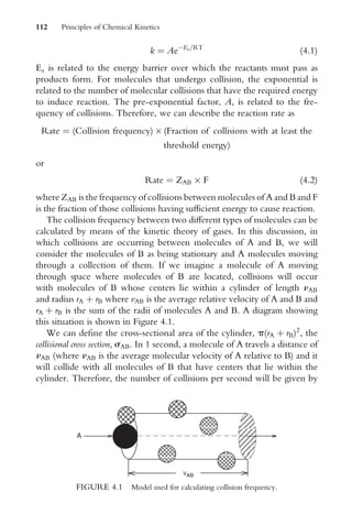


![collision energy must be suYcient, and (3) the molecules must have a
proper orientation. To compensate for the diVerence between calculated
and observed rates, a steric factor, P, is introduced. It is deWned as
P ¼
sobs
scalc
(4:14)
This steric factor can be regarded as an orientation factor but it can also be
interpreted in terms of the entropy change involved in forming the tran-
sition state.
4.2 THE POTENTIAL ENERGY SURFACE
In Chapter 1, it was shown that in one step in the reaction between H2 and
Cl2 a chlorine radical reacts with a molecule of H2. If we speculate about
the structure of this three-body species, we realize that repulsions will be
minimized if the structure is linear. Therefore, it is reasonable to assume
that the elementary reaction step can be represented as shown in the
sequence
Cl þ H-H ! [Cl H H]z
! HCl þ H
and that it passes through a linear Cl H H transition state or activated
complex. That the transition state is linear in this case follows from the fact
that to form a bent transition state would bring the terminal atoms closer
together, which would increase repulsion. To relate the energy of this
system to the bond distances is now the problem. While we might ap-
proach this problem in a number of ways, one simple approach is to extend
a relationship used for a diatomic molecule to include a second bond.
The bond energy of a diatomic molecule varies with the bond length as
shown in Figure 4.3. The energy is most favorable at the bottom of the
potential well which corresponds to the equilibrium bond length. One
equation that models the kind of relationship shown in Figure 4.3 is the
Morse equation,
E ¼ De[e2b(rro)
2eb(rro)
] (4:15)
where r is the internuclear distance, ro is the equilibrium internuclear
distance, De is the bond dissociation energy, and b is a constant. Attraction
between the atoms increases as they get closer together (the energy be-
comes more negative), but at distances smaller than ro, repulsion increases
and becomes dominant at very short internuclear distances.
116 Principles of Chemical Kinetics](https://image.slidesharecdn.com/chemicalkinetics-231126172917-d2fe5718/85/CHEMICAL-KINETICS-pdf-127-320.jpg)


![of the transition state is small because of its energy being higher than that of
the reactants, this critical conWguration represents the ‘‘regulator’’ of the
rate of Xow of reactants to products.
The concentration of the transition state is not the only factor involved,
since the frequency of its dissociation into products comes into play because
the rate at which it decomposes must also be considered. Therefore, the
rate can be expressed as
Rate ¼ Transition state concentrationÞ (Decomposition frequency)
ð
(4:20)
In order for the transition state to separate into products, one bond (the one
being broken) must acquire suYcient vibrational energy to separate. When
it does separate, one of the 3N 6 vibrational degrees of freedom (for a
linear molecule it is 3N 5) is lost and is transformed into translational
degrees of freedom of the products. Central to the idea of transition state
theory is the assumption that the transition state species is in equilibrium
with the reactants. Thus,
A þ B Ð [AB]z
! Products (4:21)
For the formation of the transition state, [AB]z
, the equilibrium constant is
Kz
¼
[AB]z
[A][B]
(4:22)
from which we Wnd that the concentration of the transition state is
[AB]z
¼ Kz
[A][B] (4:23)
Since the reaction rate is expressed as the product of the concentration of
the transition state and the frequency of its decomposition, we can now
write
Rate ¼ [AB]z
(frequency) ¼ (frequency)Kz
[A][B] (4:24)
As we have seen previously (for example, see Eq. 2.191)
Kz
¼ eDGz
=RT
(4:25)
and we know that
DGz
¼ DHz
TDSz
(4:26)
120 Principles of Chemical Kinetics](https://image.slidesharecdn.com/chemicalkinetics-231126172917-d2fe5718/85/CHEMICAL-KINETICS-pdf-131-320.jpg)
![Therefore, the equilibrium constant for formation of the transition state can
be written as
Kz
¼ eDHzTDSz
RT ¼ eDHz
RT e
DSz
R (4:27)
Substituting for Kz
in Eq. (4.24) yields
Rate ¼ (frequency)[A][B]eDHz
RT e
DSz
R (4:28)
Having obtained an expression for the rate in terms of concentrations and
thermodynamic quantities, the frequency of decomposition of transition
state must now be addressed.
If we consider the vibration of the transition state when it is at the top of
the potential energy barrier, we should now recall that the classical high-
temperature limit in energy for a vibrational mode can be expressed as
Evib ¼ kT(erg per molecule)
where k is Boltzmann’s constant and T is the temperature (K). Since
k ¼ R=No (where No is Avogadro’s number),
Evib ¼ RT( Joule per mole)
It should also be remembered that for each degree of translational freedom
the energy is kT=2, which is RT=2 per mole. If we now assume that the
frequency of the decomposition of the transition state is equal to the
frequency of the vibration being lost due to breaking a bond as products
are formed, the energy can be expressed as
E ¼ hn ¼ kT
Solving for the frequency gives
n ¼
kT
h
which can also be written as
n ¼
RT
hNo
(4:29)
Because the reaction rate can be expressed in terms of the concentration of
the transition state, the rate can now be given by
Rate ¼ k[AB]z
(4:30)
Reactions in the Gas Phase 121](https://image.slidesharecdn.com/chemicalkinetics-231126172917-d2fe5718/85/CHEMICAL-KINETICS-pdf-132-320.jpg)
![Substituting nKz
for the rate constant gives
Rate ¼ nKz
[A][B] (4:31)
When we substitute the result shown in Eq. (4.29) for the frequency in this
equation we obtain
Rate ¼
RT
hNo
Kz
[A][B] (4:32)
The rate constant can now be written as
k ¼
kT
h
Kz
¼
kT
h
eDGz
RT (4:33)
A somewhat more elegant approach to deriving an expression for the
rate of passage over the potential energy barrier is based on statistical
mechanics. According to this procedure, it is assumed that there is a certain
distance, d, at the top of the barrier, which must be the distance where the
transition state exists. It is within this distance that a vibrational mode of the
complex is transformed into translational motion of the products. The rate
of passage of the transition state through distance d is related to the
molecular velocity in one direction. If the mass of the transition state is
mz
, the average velocity is
n ¼
2kT
pmz
1=2
(4:34)
Therefore, the time required for the transition state to pass through distance
d is given by
d
v
¼ d
mz
p
2kT
1=2
(4:35)
The number of complexes crossing the potential barrier through distance
d per unit time is
d[ z ]
dt
¼
[ z ]
2
d
pmz
2kT
1=2
¼
[ z ]
d
kT
2pmz
1=2
(4:36)
Note that we are using [ ]z
to represent the transition state and [z] to
represent the concentration of the transition state. Now, the concentration
122 Principles of Chemical Kinetics](https://image.slidesharecdn.com/chemicalkinetics-231126172917-d2fe5718/85/CHEMICAL-KINETICS-pdf-133-320.jpg)
![of the transition state, [z], is to be evaluated. If the diVerence between the
zero-point energies of the reactants and the transition state is represented as
Eo
z
, the equilibrium constant for formation of the transition state is given
by
Kz
¼
Qz
QAQB
eEo
z
RT (4:37)
where QA,QB, and Qz
are the partition functions of reactants A and B and
the transition state, respectively. If the vibrational mode of the transition
state is factored out of Q we can write
Qz
¼ Qz0
qz
v (4:38)
where qz
v is the vibrational mode of the bond being broken. Now we can
approximate the vibrational mode as
qz
v ¼
1
1 ehn
kT
¼
kT
hnz
(4:39)
and the equilibrium constant Kz
is given by
Kz
¼
kT
hnz
Qz0
QAQB
eEo
z
RT (4:40)
which is of the same form found earlier with the rate constant, k, being
given by
k ¼
kT
h
Qz0
QAQB
eEo
z
RT (4:41)
The resemblance of this equation to the Arrhenius equation is apparent
when the pre-exponential factor includes the frequency factor and the
equilibrium constant in terms of partition functions. This expression for k
is similar to that obtained from collision theory.
An approximate rate constant, ka, can be calculated from probability that
the reactants in the distribution of quantum state will collide and react in
accord with the collision frequency. The approximate constant is greater
than the measured rate constant, k. One approach to improving transition
state theory with respect to calculating the rate constant is to alter the
conWguration of the transition state used in the energy calculations in order
to eVect a change in ka. In fact, the calculations are performed in such a way
that the calculated rate constant is a minimum and thereby approaches the
observed k. Just as energy minimization is accomplished by means of the
Reactions in the Gas Phase 123](https://image.slidesharecdn.com/chemicalkinetics-231126172917-d2fe5718/85/CHEMICAL-KINETICS-pdf-134-320.jpg)

![raising the translational and vibrational energy of the second molecule. The
activation of molecules by collision can thus be accomplished. However,
the activated molecule need not react immediately, and, in fact, it may
become deactivated by undergoing subsequent collisions before it reacts.
For reaction to occur, the activated molecule that has increased vibrational
energy must have some bond activated to the point where bond rupture
occurs.
The elementary reactions by which A is converted into products can be
shown as
A þ A Ð
k1
k1
A þ A
(4:45)
A
!
k2
Products (4:46)
In this scheme, A
is the activated molecule of A. Although the process
producing A
is bimolecular, the decomposition of A
is unimolecular. The
change in [A] with time can be expressed by the equation
d[A]
dt
¼ k1[A]2
k1[A][A
] (4:47)
Since A
is an activated molecule, a reactive intermediate, the steady state
approximation is assumed to apply (see Section 2.4). The rate of formation
of A
is assumed to be equal to its rate of decomposition. Therefore,
d[A]
dt
¼ 0 ¼ k1[A]2
k1[A][A
] k2[A
] (4:48)
The Wrst term on the right-hand side of the equation represents the rate of
activation of A while the second and third terms represent deactivation and
decomposition of A
, respectively. Solving Eq. (4.48) for [A
], we obtain
[A
] ¼
k1[A]2
k1[A] þ k2
(4:49)
Substituting this result in Eq. (4.47), we obtain
d[A]
dt
¼
k1k2[A]2
k1[A] þ k2
(4:50)
At high pressures, the number of A molecules per unit volume is large, and
deactivation of A
can occur by frequent collisions with other molecules
of A. Under these conditions, we will consider the rate of deactivation
Reactions in the Gas Phase 125](https://image.slidesharecdn.com/chemicalkinetics-231126172917-d2fe5718/85/CHEMICAL-KINETICS-pdf-136-320.jpg)
![of A
to be large compared to the rate of decomposition. Therefore,
k1[A] k2 and
d[A]
dt
¼
k1k2[A]2
k1[A] þ k2
k1k2[A]2
k1[A]
¼ k[A] (4:51)
where k ¼ k1k2=k1. Therefore, at relatively high pressure where [A] is
high, the reaction appears to be unimolecular (Wrst-order) in [A].
At low pressures of A, the rate of decomposition of A
is greater than the
rate of its deactivation by collision with A because there are fewer mol-
ecules of A available. Under these conditions, the increase in vibrational
energy can cause bond rupture and decomposition. Therefore, in this case,
k2 k1[A] and
d[A]
dt
¼
k1k2[A]2
k2
¼ k1[A]2
(4:52)
This equation shows that at low pressures of the reacting gas, the reaction
should be bimolecular (second-order). Thus, the observed bimolecular
dependence at low pressure and the unimolecular dependence at high
pressure are predicted by a mechanism involving activation of molecules
by collision.
The activation of reactant molecules by collision was described earlier.
However, this is not the only vehicle for molecular activation. It is possible
for a non-reactant gas (a so-called third body) to cause activation of
molecules of the reactant. If we represent such a species by M, the processes
of activation, deactivation, and product production are given by
A þ M Ð
k1
k1
A
þ M (4:53)
A
!
k2
Products (4:54)
Therefore, the rate of disappearance of A can be written as
d[A]
dt
¼ k1[A][M] k1[A
][M] (4:55)
The net change in concentration of A
with time is given by the diVerence
between the rate at which it is formed as represented in Eq. (4.53) and the
rate at which it is removed by undergoing reaction as shown in Eq. (4.54).
d[A
]
dt
¼ k1[A][M] k1[A
][M] k2
[A
] ¼ 0 (4:56)
126 Principles of Chemical Kinetics](https://image.slidesharecdn.com/chemicalkinetics-231126172917-d2fe5718/85/CHEMICAL-KINETICS-pdf-137-320.jpg)
![Therefore, rearrangement gives
0 ¼ k1[A][M] (k1[M] þ k2)[A
] (4:57)
and solving for [A
] yields
[A
] ¼
k1[A][M]
k1[M] þ k2
(4:58)
Substituting for [A
] in Eq. (4.55) gives
d[A]
dt
¼ k1[A][M] k1[M]
k1[A][M]
k1[M] þ k2
(4:59)
Factoring out the quantity k1[A][M] on the right-hand side enables us to
write this equation in the form
d[A]
dt
¼ k1[A][M] 1
k1[M]
k1[M] þ k2
(4:60)
The quantity inside the parentheses can be made into a single fraction
to give
d[A]
dt
¼ k1[A][M]
k1[M] þ k2
k1[M] þ k2
k1[M]
k1[M] þ k2
(4:61)
This equation can now be written as
d[A]
dt
¼ k1[A][M]
k1[M] þ k2 k1[M]
k1[M] þ k2
(4:62)
and simpliWed to obtain
d[A]
dt
¼
k1k2[M][A]
k1[M] þ k2
(4:63)
The results obtained by considering activation by a third body must now be
compared to those described earlier for activation by collision of reactant
molecules.
At high pressure, the rate of deactivation by collisions with M is likely to
be greater than the rate of reaction, so k1[M] k2 and neglecting k2 in
the denominator of Eq. (4.63) gives
d[A]
dt
k1k2[M][A]
k1[M]
k0
[A] (4:64)
Reactions in the Gas Phase 127](https://image.slidesharecdn.com/chemicalkinetics-231126172917-d2fe5718/85/CHEMICAL-KINETICS-pdf-138-320.jpg)
![This approximation shows that the reaction follows a Wrst-order rate law.
At low pressure, the concentration of M is low, so k1[M] k2 and
d[A]
dt
k1k2[M][A]
k2
k1[A][M] (4:65)
Therefore, the reaction appears to be Wrst-order in A and Wrst-order in M.
If the species M is simply another molecule of reactant A, this equation
becomes
d[A]
dt
¼ k1[A]2
(4:66)
which is the second-order rate expression found earlier. These results are in
accord with experience for the unimolecular decomposition of a large
number of gaseous compounds.
Ozone decomposes by a mechanism that appears to be somewhat
diVerent from that described earlier, but it provides a rather simple appli-
cation of the steady state approximation. The overall reaction is
2O3( g) ! 3O2( g) (4:67)
for which the observed rate law is
d[O3]
dt
¼
k[O3]2
[O2]
(4:68)
Therefore, the reaction is second-order in ozone but the reaction is
inhibited by O2. This reaction is believed to involve a third body (an
inert molecule or particle) in the steps
O3( g) þ M Ð
k1
k1
O2( g) þ O( g) þ M (fast) (4:69)
O( g) þ O3( g)
!
k2
2O2( g) (slow) (4:70)
The rate constant for the second reaction is much smaller than that for the
Wrst, so the second reaction is rate determining. Therefore, the rate equa-
tion is written as
d[O3]
dt
¼ k2[O][O3] (4:71)
The rate of O formation is given by
d[O]
dt
¼ k1[M][O3] (4:72)
128 Principles of Chemical Kinetics](https://image.slidesharecdn.com/chemicalkinetics-231126172917-d2fe5718/85/CHEMICAL-KINETICS-pdf-139-320.jpg)
![and the rate of consumption of O is
d[O]
dt
¼ k1[M][O][O2] (4:73)
Therefore, applying the steady state approximation,
k1[M][O3] ¼ k1[M][O][O2] (4:74)
Solving this equation for [O] we obtain
[O] ¼
k1[O3]
k1[O2]
(4:75)
which when substituted in Eq. (4.71) gives
d[O3]
dt
¼ k2[O3]
k1[O3]
k1[O2]
¼ k
[O3]2
[O2]
(4:76)
This is the form of the observed rate law where k ¼ k1k2=k1.
The approach of Lindemann is based on collisional activation of mol-
ecules as a result of energy transfer. C. N. Hinshelwood (Nobel Prize in
1956) extended this approach to include changes in vibrational energies
that can be distributed internally to supply suYcient energy to the bond
being broken. This approach provided a better Wt to observed kinetics in
the region of low pressure.
In the late 1920s, O. K. Rice and H. C. Ramsperger as well as L. S.
Kassel developed an approach (now known as the RRK theory) to unim-
olecular decomposition reactions which is based on statistically treating the
molecules as coupled oscillators. In this way, energy is presumed to be
distributed about the energized molecule until it vibrates in a way that
results in bond rupture. In this treatment, it is assumed that the amount of
energy, E
, must be localized in the bond being broken and that the
probability of this happening is given by
P ¼
E E
E
N1
(4:77)
where N is the number of vibrational modes (3N 5 for linear molecules
and 3N 6 for nonlinear molecules). The rate constant is presumed
proportional to the probability, so it is given by
k ¼
E E
E
N1
(4:78)
Reactions in the Gas Phase 129](https://image.slidesharecdn.com/chemicalkinetics-231126172917-d2fe5718/85/CHEMICAL-KINETICS-pdf-140-320.jpg)
![It can then be shown that at high pressure
k ¼ eE
=kT
(4:79)
A later modiWcation of the RRK theory presented by R. A. Marcus ( J.
Chem. Phys., 1952, 20, 359) (Nobel Prize in 1992) resulted in the so-called
RRKM theory. In this case, the mechanism of the reaction consists of the
following steps
A þ M Ð
k1
k1
A
þ M (4:80)
A
!
k2
Az
(4:81)
Az
!
k3
Products (4:82)
The essential idea is that the activated molecule, A
, becomes the transition
state or activated complex, Az
, which then leads to product formation. This is
presumed to occur when the energy at the reactive site becomes as large as
Ea, the activation energy. The rate at which A
is transformed into A
depends on the number of degrees of vibrational freedom. Therefore, the
theory is concerned with the treatment of the vibrational frequencies of A
and A in the calculations.
From the preceding processes, we can write the rate law
d[A]
dt
¼ k1[A][M] k1[A
][M] (4:83)
Applying the steady state approximation with regard to A
gives
d[A
]
dt
¼ k1[A][M] k1[A
][M] k2[A
] ¼ 0 (4:84)
Therefore, the concentration of A
can be expressed as
[A
] ¼
k1[A][M]
k2 þ k1[M]
(4:85)
From Eq. (4.84), we Wnd that
k1[A
][M] ¼ k1½A ½M k2½A
(4:86)
Therefore, substituting for k1[A
][M] in Eq. (4.83) yields
d[A]
dt
¼ k1[A][M] k1[A
][M] ¼ k1[A][M] (k1[A][M] k2[A
])
(4:87)
130 Principles of Chemical Kinetics](https://image.slidesharecdn.com/chemicalkinetics-231126172917-d2fe5718/85/CHEMICAL-KINETICS-pdf-141-320.jpg)
![which can be simpliWed to obtain
d[A]
dt
¼ k2[A
] (4:88)
Now, substituting the expression shown in Eq. (4.85) for [A
] gives
d[A]
dt
¼
k1k2[A][M]
k2 þ k1[M]
¼
k1k2[M]
k2 þ k1[M]
[A] (4:89)
We can now consider the quantity in brackets as the rate constant for the
formation of product or disappearance of A. If k1[M] k2, the equation
reduces to
d[A]
dt
¼ k0
[A] (4:90)
where k0
¼ k1k2=k1 and the reaction appears to be Wrst-order in A. If
k2 k1[M], the rate shown in Eq. (4.89) becomes
d[A]
dt
¼ k1[A][M] (4:91)
and, when the third body, M, is a second molecule of A, the equation
becomes
d[A]
dt
¼ k1[A]2
(4:92)
Therefore, the reaction shows a second-order dependence on A. Many of the
details of the Marcus theory can be found in the book by Nicholas (1976).
4.5 FREE RADICAL OR CHAIN MECHANISMS
Some of the elementary concepts of free radical mechanisms were pre-
sented in Chapter 1. Reactions following free radical mechanisms have
reactive intermediates containing unpaired electrons which are produced
by homolytic cleavage of covalent bonds. A method of detecting free
radicals was published in 1929, and it is based on the fact that metals such
as lead react with free radicals. When heated, tetramethyl lead decomposes,
(CH3)4Pb ! Pb þ 4 CH3 (4:93)
A lead mirror is produced in a heated glass tube when tetramethyl lead is
passed through it. Also, the lead mirror in a cool portion of the tube can be
Reactions in the Gas Phase 131](https://image.slidesharecdn.com/chemicalkinetics-231126172917-d2fe5718/85/CHEMICAL-KINETICS-pdf-142-320.jpg)
![removed by passing tetramethyl lead through a hot potion of the tube Wrst
to produce CH3 radicals. In the cool portion of the tube, the reaction is
4 CH3 þ Pb ! (CH3)4Pb (4:94)
However, if the Xow system is arranged so that a long tube is used and
considerable distance separates the point where the CH3 radicals are
generated and they react with the cool lead mirror, the reaction is hindered
because of radical recombination.
2 CH3 ! C2H6 (4:95)
Perhaps the best known example of a chain process, certainly it is the
classic case, is the reaction
H2 þ Br2 ! 2 HBr (4:96)
This reaction was studied by Bodenstein and Lind nearly 90 years ago, and
the rate law found was written as
d[HBr]
dt
¼
k[H2][Br2]1=2
1 þ k0
[HBr]
[Br2]
(4:97)
where k and k0
are constants with k0
¼ 10. The [HBr] in the denominator
indicates that the rate is decreased as [HBr] increases so that HBr functions
as an inhibitor. The reaction has now been studied both thermally and
photochemically and the initiation step is now agreed to be
Br2 ! 2 Br (4:98)
The overall reaction scheme was postulated in 1919 by Christiansen,
Herzfeld, and Polyani in three separate publications.
The overall process is now described in terms of the elementary steps
Br2
!
k1
2 Br (4:99)
Br þ H2
!
k2
HBr þ H (4:100)
H þ Br2
!
k3
HBr þ Br (4:101)
H þ HBr
!
k4
H2 þ Br (4:102)
2 Br
!
k5
Br2 (4:103)
132 Principles of Chemical Kinetics](https://image.slidesharecdn.com/chemicalkinetics-231126172917-d2fe5718/85/CHEMICAL-KINETICS-pdf-143-320.jpg)
![SimpliWcation of the mathematical problem is achieved by application of
the steady state hypothesis to those species that occur only in the propaga-
tion steps. In this case, it is assumed that [Br] and [H] are at some low,
essentially constant level. Therefore,
d[Br]
dt
¼ 0 and
d[H]
dt
¼ 0 (4:104)
Following the same type of treatment as was used in cases described in
Chapter 2, we express [Br] and [H] in terms of their rates of formation
and disappearance. Therefore, for simplicity using [H] and [Br] instead of
[H] and [Br], we can write the equation giving the change in concentra-
tion of H with time from the preceding elementary steps as
d[H]
dt
¼ k2[Br][H2] k3[H][Br2] k4[H][HBr] ¼ 0 (4:105)
The equation giving the change in concentration of Br with time can be
written as
d[Br]
dt
¼ 2k1[Br2] k2[Br][H2] þ k3[H][Br2] þ k4[H][HBr] 2k5[Br]2
¼ 0
(4:106)
Now we can also write the equation that gives the production of HBr as
d[HBr]
dt
¼ k2[Br][H2] þ k3[H][Br2] k4[H][HBr] (4:107)
If we subtract Eq. (4.105) from Eq. (4.107), while letting d[H]=dt ¼ 0,we
obtain
d[HBr]
dt
0 ¼ k2[Br][H2] þ k3[H][Br2] k4[H][HBr]
{k2[Br][H2] k3[H][Br2] k4[H][HBr]} (4:108)
SimpliWcation of this equation leads to
d[HBr]
dt
¼ 2k3[H][Br2] (4:109)
Adding Equations (4.105) and (4.106) gives
0 ¼ k2[Br][H2] k3[H] ]Br2] k4[H][HBr] þ 2k1[Br2]
k2[Br][H2] þ k3[H][Br2] þ k4[H][HBr] 2k5[Br]2
(4:110)
Reactions in the Gas Phase 133](https://image.slidesharecdn.com/chemicalkinetics-231126172917-d2fe5718/85/CHEMICAL-KINETICS-pdf-144-320.jpg)
![which can be simpliWed to give
2k1[Br2] 2k5[Br]2
¼ 0 (4:111)
Solving this equation for [Br] yields
[Br] ¼ {(k1=k5)[Br2]}1=2
(4:112)
Substitution of this value for [Br] in Eq. (4.105) gives
k2[Br][H2] k3[H][Br2] k4[H][HBr] ¼ k2{(k1=k5)[Br2]}1=2
[H2]
k3[H][Br2] k4[H][HBr] ¼ 0 (4:113)
k2{(k1=k5)[Br2]}1=2
[H2] [H](k3[Br2] k4[HBr]) ¼ 0 (4:114)
Solving this equation for [H] yields
[H] ¼
k2
k1
k5
[Br2]
1=2
[H2]
k3[Br2] þ k4[HBr]
(4:115)
Substituting this result for [H] in Eq. (4.109) we obtain
d[HBr]
dt
¼ 2k3[H][Br2] ¼
2k2k3
k1
k5
[Br2]
1=2
[H2][Br2]
k3[Br2] þ k4[HBr]
(4:116)
This equation can be simpliWed to obtain
d[HBr]
dt
¼
2k2k3
k1
k5
1=2
[H2][Br2]3=2
k3[Br2] þ k4[HBr]
(4:117)
Dividing numerator and denominator of the right-hand side of this equa-
tion by k3[Br2] gives
d[HBr]
dt
¼
2k2
k1
k5
1=2
[H2][Br2]1=2
1 þ
k4[HBr]
k3[Br2]
(4:118)
If we let k ¼ 2k2(k1=k5)1=2
and k0
¼ k4=k3, Eq. (4.118) has the same form as
the empirical rate law shown in Eq. (4.97). We need now to examine the
relationships between the rate constants. The bond energies for the
molecular species in Steps 3 and 4 (Eqs. (4.101) and (4.102)) are as follows:
134 Principles of Chemical Kinetics](https://image.slidesharecdn.com/chemicalkinetics-231126172917-d2fe5718/85/CHEMICAL-KINETICS-pdf-145-320.jpg)
![HH, 436; BrBr, 193; and HBr, 366 kJ=mol. Therefore, both Steps 3
and 4 are exothermic having enthalpies of about 173 and 70 kJ=mol,
respectively. Activation energies for forming the transition states
[H Br Br] and [H H Br] are very low so there will be almost no
temperature dependence on the rates of their formation and the tempera-
ture eVects will approximately cancel. Therefore, the ratio k4=k3 is con-
stant, having a value of 10.
Other reactions in the chain process could conceivably include
H2 ! 2 H (4:119)
but the bond energy for H2 is about 436 kJ=mol while that for Br2 is
193 kJ=mol. Consequently, any dissociation involving H2 would be
insigniWcant compared to the dissociation of Br2. Likewise, the dissociation
of HBr to give H and Br would be energetically unfavorable as would the
reaction
Br þ HBr ! H þ Br2 (4:120)
Finally, the reactions
H þ H ! H2 (4:121)
H þ Br ! HBr (4:122)
can be considered as unlikely at best owing to the very low stationary state
concentrations of these H radicals. There are other arguments against these
processes as well.
Radicals are generated, consumed, or propagated by a relatively few
types of elementary reactions. Radical generation usually involves the
homolytic dissociation of some covalent bond.
X Y
!
X þ
Y (4:123)
In this case, the process is a high-energy one so it is usually brought about
by thermal, photochemical, or electrical means. The consumption of
radicals occurs in termination steps, which include processes like
Br þ Br ! Br2 (4:124)
CH3 þ CH3 ! C2H6 (4:125)
The propagation of radicals can involve a transfer of atoms, which can be
shown as
XY þ Z ! XZ þ Y (4:126)
Reactions in the Gas Phase 135](https://image.slidesharecdn.com/chemicalkinetics-231126172917-d2fe5718/85/CHEMICAL-KINETICS-pdf-146-320.jpg)


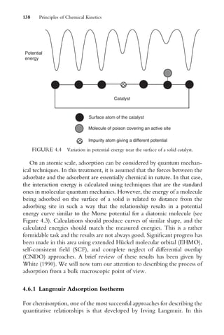


![Nicholas, J. (1976). Chemical Kinetics, Wiley, New York, Chapters 2, 5, 6, and 7. A clear,
thorough coverage of gas phase reaction kinetics.
Pilling, M. J., Seakins, P. W. (1996). Reaction Kinetics, Oxford University Press, New York.
Steinfeld, J. I., Francisco, J. S., Hase, W. L. (1998). Chemical Kinetics and Dynamics, 2nd Ed.,
Prentice Hall, Upper Saddle River, NJ.
Truhlar, D.G., Garrett, B.C. (1980). Acc. Chem. Res., 13, 440.
White, M. G. (1990). Heterogeneous Catalysis, Prentice Hall, Englewood CliVs, NJ Chapters
1, 3, 7, 8, and 9. Detailed coverage of the subject.
PROBLEMS
1. Unimolecular decompositions can appear to be Wrst- or second-order
under certain conditions. What assumptions were applied to the solu-
tion of this problem? Write out the mechanism for the unimolecular
decomposition of X(g) and derive the rate law. Explain how this rate law
accounts for the observations on reaction order.
2. Suppose that a reaction follows the scheme
X
!
k1
R
R þ X
!
k2
P þ 2 R
R
!
k3
Z
What is a reaction scheme like this called? Derive the rate expression
giving [R] as a function of time. Using your derived rate expression,
explain what can happen when the concentration of X is varied between
rather wide limits. What type of chemical event does this correspond to?
3. Consider the decomposition of CH3CHO into CH4 and CO, which is
believed to take place in the steps
CH3CHO
!
k1
CH3 þ CHO
CH3 þ CH3CHO
!
k2
CH4 þ CO þ CH3
2 CH3
!
k3
C2H6
Use the steady state approximation to derive the rate law for the
formation of CH4. What would the rate of formation of CO be?
148 Principles of Chemical Kinetics](https://image.slidesharecdn.com/chemicalkinetics-231126172917-d2fe5718/85/CHEMICAL-KINETICS-pdf-159-320.jpg)
![4. The rate of the reaction
H2( g) þ I2( g) ! 2 HI( g)
is increased by electromagnetic radiation. Assuming that the radiation
rapidly separates I2 into I and that the equilibrium
I þ H2( g) Ð IH2( g)
is reached rapidly, the slow step in the process is believed to be
IH2 þ I( g) ! 2 HI( g)
Show that this mechanism is consistent with a rate law of the form
Rate ¼ k[H2][I2]
5. For the reaction
2NO2Cl( g) ! 2NO2( g) þ Cl2
one possible mechanism is
NO2Cl ! NO2 þ Cl
Cl þ NO2Cl ! NO2 þ Cl2
The observed rate law is Rate ¼ [NO2Cl]. What does this tell about the
mechanism?
6. Derive the rate law for the process represented by the following mech-
anism.
A Ð
k1
k1
B þ X (fast)
X þ D Ð
k2
k2
E (fast)
E
!F (slow)
7. Consider the reaction scheme
NO( g) þ H2( g) Ð
k1
k1
H2ON( g) (fast)
Reactions in the Gas Phase 149](https://image.slidesharecdn.com/chemicalkinetics-231126172917-d2fe5718/85/CHEMICAL-KINETICS-pdf-160-320.jpg)
![H2ON( g) þ NO( g)
!
k2
N2( g) þ H2O2( g) (slow)
H2O2( g) þ H2( g)
!
k3
2H2O( g) (fast)
Write the rate law for the overall reaction in terms of the steps just given.
Apply the steady state approximation and obtain the Wnal rate law.
8. The reaction between H2 and Br2 has been described in terms of these
steps:
Br2
!
k1
2Br
Br þ H2
!
k2
HBr þ H
H þ Br2
!
k3
HBr þ Br
H þ HBr
!
k4
H2 þ Br
Write the rate laws for the change in concentration of H, Br, and
HBr with time. Apply the steady state approximation and show that
the rate of formation of HBr is
d[HBr]
dt
¼
k1
k1
1=2
2k2[H2][Br2]1=2
1 þ
k4
k3
[HBr]
[Br2]
9. For each of the following, use the Langmuir isotherm and provide an
interpretation for the observation. (a) The decomposition of gas X on
solid S is zero-order. (b) The decomposition of gas Y on solid S is Wrst-
order. (c) The decomposition of NH3 on a platinum surface is in-
versely proportional to the pressure of H2 and directly proportional to
the pressure of NH3.
10. The reaction of NO(g) with Br2( g) produces ONBr(g) and may take
place in the steps
NO( g) þ Br2( g) Ð
k1
k1
ONBr2( g) (fast)
ONBr2( g) þ NO( g)
!
k2
2ONBr( g) (slow)
150 Principles of Chemical Kinetics](https://image.slidesharecdn.com/chemicalkinetics-231126172917-d2fe5718/85/CHEMICAL-KINETICS-pdf-161-320.jpg)
![Assuming that ONBr2( g) establishes a steady state concentration,
derive the rate law for the production of ONBr(g).
11. Suppose a gaseous reaction takes place in the steps
A Ð
k1
k1
B
B þ C
!
k2
D
Derive the rate law for the formation of D and show the limiting forms
at high pressure and low pressure.
12. The decomposition of tetraborane-10, B4H10, is thought to take place
in the following steps (Bond, A. C., Pinsky, M. L., J. Am. Chem. Soc.
1970, 92, 32).
B4H10
!
k1
B3H7 þ BH3
B3H7
!
k2
BH2 þ B2H5
B2H5
!
k3
BH2 þ BH3
BH2 þ B4H10
!
k4
B4H9 þ BH3
B4H9
!
k5
B2H5 þ B2H4
B2H4
!
k6
H2 þ solid product
2 BH2
!
k7
B2H4
2 BH3
!
k8
B2H6
Make the steady state assumption regarding BH2,BH3,B2H4,B2H5,
B3H7, and B4H9, and show that the rate law is
d[[B4H10]
dt
¼ k1[B4H10] þ
k4(2k1)1=2
k
1=2
7
[B4H10]3=2
13. The decomposition of N2O5 is believed to involve the following steps.
N2O5 Ð
k1
k1
NO2 þ NO3
Reactions in the Gas Phase 151](https://image.slidesharecdn.com/chemicalkinetics-231126172917-d2fe5718/85/CHEMICAL-KINETICS-pdf-162-320.jpg)


![unable to interact with each other. In other words, the interaction between
molecules of the solute and solvent will compete with interactions between
the solute molecules. Thus, the association of a polar solute can be shown as
2D Ð D2 (5:5)
for which the equilibrium constant K ¼ [D2]=[D]2
will be strongly solvent
dependent. In the same way that interactions between ions are governed by
Coulomb’s law, the dielectric constant of the solvent will aVect the attrac-
tion between dipoles. Species that are of extreme diVerence in polarity may
not be completely miscible owing to each type of molecule interacting
strongly with molecules of its own kind. Although they are weak compared
to chemical bonds, dipole-dipole forces are of considerable importance in
determining chemical properties.
A permanent dipole, m ¼ q r can induce a charge separation in a
neighboring nonpolar molecule that is proportional to the polarizability
of the molecule. If the polarizability of the molecule is represented as a, the
energy of the interaction between the permanent dipole and the nonpolar
molecule with an induced dipole moment can be expressed as
EI ¼
2am2
r6
(5:6)
These forces between polar molecules and those having a dipole induced in
them are called dipole-induced dipole forces, and they are essentially tempera-
ture independent.
It should be apparent that there must be some force between molecules
that are nonpolar because CH4, He, CO2, and similar molecules can be
liqueWed. These forces must also be electrical in nature but cannot be the
result of an overall charge separation within the molecules. If we consider
two helium atoms as shown in Figure 5.1, it is possible that at some instant
both of the electrons in one atom will be on the same side of the atom.
There is an instantaneous dipole that will cause an instantaneous change in
+
− +
−
FIGURE 5.1 Two helium atoms showing the instantaneous dipoles that result in a weak
force of attraction.
156 Principles of Chemical Kinetics](https://image.slidesharecdn.com/chemicalkinetics-231126172917-d2fe5718/85/CHEMICAL-KINETICS-pdf-167-320.jpg)


![Because the solubility parameter reXects the intermolecular forces in a
liquid, it is a very useful parameter. The total interaction between mol-
ecules in a liquid may be the result of dipole-dipole, London, and hydro-
gen-bonding interactions. Therefore, it is possible to separate the
contributions from each type of interaction and express the solubility
parameter as though it were a vector sum. The result is
d2
¼ d2
L þ d2
D þ d2
H (5:28)
where dD, dL, and dH are contributions to the solubility parameter from
dipole-dipole, London, and hydrogen-bonding interactions, respectively.
5.1.3 Solvation of Ions and Molecules
When an ionic compound dissolves in a polar solvent such as water, the
ions become strongly solvated. The ion-dipole forces produce a layer of
solvent molecules (the primary solvation sphere) surrounding each ion.
This layer can cause other solvent molecules in the immediate vicinity to
become oriented as well. Although the primary solvation sphere may seem
to be rather Wrmly attached to the ion, there is considerable interchange
between these molecules and the bulk solvent in a dynamic process in most
cases. For strongly solvated ions like [Cr(H2O6]3þ
, the exchange of coord-
inated water molecules and those of the bulk solvent is very slow. As we
shall describe later, some desolvation of ionic species may be required
before a reaction of the ion can take place.
The nature of solvated species is often an important consideration. For
example, the symbol for the solvated proton in acidic solutions is written as
H3Oþ
, but the Hþ
is solvated by more than one water molecule. In fact,
the predominant species is probably H9O4
þ
, which is Hþ4H2O, and this
ion has been identiWed in vapors above concentrated acids as well as a
cation in solids, so it has some stability. Other species (e.g., H7O3
þ
, which
is Hþ
solvated by three H2O molecules) can also exist in equilibrium with
H9O4
þ
. In general, the average number of water molecules solvating an
ion depends on the concentration of the ion in the solution as well as the
size and charge of the ion.
Theoretical treatment of the solvation of ions is quite diYcult. If we
could use a simple electrostatic approach in which polar molecules interact
with a charged ion, the problem would be much simpler. However, the
fact that the polar solvent molecules interact with an ion causes their
Reactions in Solutions 163](https://image.slidesharecdn.com/chemicalkinetics-231126172917-d2fe5718/85/CHEMICAL-KINETICS-pdf-174-320.jpg)


![5.6 SOLVATION AND ITS EFFECTS ON RATES
The complexity of reactions in solution has already been described brieXy.
However, many unimolecular reactions have rates in solutions that are
approximately equal to those in the gas phase. The population of the
transition state depends on the number of critical vibrational states popu-
lated, which is a function of temperature rather than the environment of
the reacting molecule. The localization of the required energy in a vibra-
tional mode for a bond to be broken is often somewhat independent of the
environment of the molecule.
Generally, reacting molecules must come together and collide, form a
transition state and react, and allow the products to be removed by diVusion
from the reaction zone. In viscous media, the collision frequency of the
reactants may limit the rate of formation of the transition state as a result of
slow diVusion.
Consider a process in which two solvated reactant molecules A and B
must come together to form a transition state. This process can be con-
sidered as requiring close proximity of A and B (sometimes called a collision
complex) followed by the formation of the actual critical conWguration in
space, which is the reactive transition state. This process can be shown as
follows.
A(solv) þ B(solv)
!
kc
AB(solv)
!
ka
[TS]z
(solv) (5:70)
In this scheme, AB(solv) is the solvated collision complex of A and B, while
[TS]z
(solv) is the solvated transition state. We can characterize the rate of
formation of the collision complex by the rate constant kc and that of the
formation of the transition state by ka. The rate of diVusion of A and B in
the solution determines kc, and there is an activation energy associated with
that process. In an approximate way, the activation energy for diVusion can
be considered as having a lower limit that is on the order of the activation
energy for viscous Xow of the solvent. Such energies are generally lower
than those required to form transition states during chemical reactions.
Therefore, kc ka, and the formation of the transition state is the rate-
determining process. In the case of very viscous solvents and strong solv-
ation of reactants A and B, the formation of the collision complex of A and
B may be the rate-determining factor. In this case, the rate of the reaction is
limited by the rate of formation of the collision complex, and the reaction is
said to be diVusion controlled.
Reactions in Solutions 177](https://image.slidesharecdn.com/chemicalkinetics-231126172917-d2fe5718/85/CHEMICAL-KINETICS-pdf-188-320.jpg)
![Although diVusion controlled reactions constitute a diYcult special case,
a general comparison of the behavior of gas phase reactions with those
taking place in solution needs to be made. A problem with doing this is
that few reactions that occur in the gas phase can be studied in solution
under conditions that are otherwise the same with respect to temperature,
concentration, etc. In some cases, even the products of the reaction may
be diVerent. The majority of studies on solvent eVects have dealt with
investigating the diVerences in kinetics of a reaction when diVerent solvents
are used rather than comparing the rates of gas phase reactions with those
taking place in a solvent.
Let us consider the reaction between A and B that takes place in the gas
phase and in some solvent to form the same products. We will write the
process in the two phases as follows.
A(g) B(g)
+ [TS]‡
(g) Products
A(solv) B(solv)
+ Products
[TS]‡
(solv)
∆G‡ (solv)
∆GB (solv)
∆GA (solv)
k1g
k–1g
k1s
k–1s
If the transition states formed under the two sets of conditions are identical
except for solvation and have equal probabilities for reaction, the rate of the
reaction in each case will be determined only by the concentration of the
transition state. Therefore,
Rate [TS]z
(5:71)
For the reaction in the gas phase,
Rg [TS]z
g ¼ Kz
g[A]g[B]g (5:72)
and for the reaction in solution,
Rs [TS]z
s ¼ Kz
s [A]s[B]s (5:73)
where Kz
g and Kz
s are the equilibrium constants for the formation of the
transition states in the gas phase and in solution. Therefore, when the
concentrations of A and B are identical in the two phases, the ratio of the
rates is given by the ratio of the equilibrium constants,
Rg
Rs
¼
Kz
g
Kz
s
(5:74)
178 Principles of Chemical Kinetics](https://image.slidesharecdn.com/chemicalkinetics-231126172917-d2fe5718/85/CHEMICAL-KINETICS-pdf-189-320.jpg)

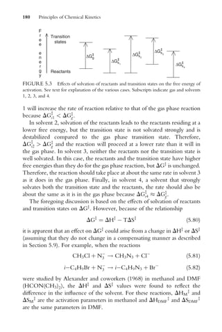

![5.7 EFFECTS OF IONIC STRENGTH
When ions react in solution, their charges result in electrostatic forces that
aVect the kinetics of the reactions. We can see how this situation arises in
the following way. If a reaction occurs between a cation having a charge ZA
and an anion having a charge of ZB, the transition state will be [AB]ZAþZB
.
The equilibrium constant for the formation of the transition state can be
written in terms of the activities of the species as
Kz
¼
az
aAaB
¼
[TS]z
gz
[A]gA[B]gB
(5:83)
where a is an activity and g is an activity coeYcient. From this equation, we
obtain
[TS]z
¼
Kz
gAgB[A][B]
gz
(5:84)
For the reaction A ! B, the rate of the reaction can be written as
d[A]
dt
¼ k[TS]z
¼ kKz
[A][B]
gAgB
gz
(5:85)
When written in terms of the frequency of the decomposition of the
transition state, n, which is equal to kT=h, the rate equation becomes
d[A]
dt
¼
kT
h
gAgB
gz
(5:86)
If the solution is suYciently dilute so that the Debye-Hückel limiting law
applies,
log gi ¼ 0:509Z2
i I1=2
(5:87)
where Zi is the charge on the species and I is the ionic strength of the
solution. Therefore,
log k ¼ log
kT
h
Kz
þ log
gAgB
gz
(5:88)
which by expanding the term containing the activity coeYcients can be
written as
log k ¼ log
kT
h
Kz
þ log gA þ log gB log gz (5:89)
182 Principles of Chemical Kinetics](https://image.slidesharecdn.com/chemicalkinetics-231126172917-d2fe5718/85/CHEMICAL-KINETICS-pdf-193-320.jpg)
![Substituting for the terms containing log g gives
log k ¼ log
kT
h
Kz
0:509(Z2
A þ Z2
B Z2
z )I1=2
(5:90)
The charge on the transition state [TS]z
is ZA þ ZB, so
Z2
z ¼ (ZA þ ZB)2
¼ Z2
A þ Z2
B þ 2ZAZB (5:91)
Therefore, when this result is substituted in Eq. (5.90), after simpliWcation
we obtain
log k ¼ log
kT
h
Kz
þ 1:018ZAZBI1=2
(5:92)
When the Wrst term on the right-hand side of this equation is represented as
ko, this equation can be written in logarithmic form as
log
k
ko
¼ 1:018ZAZBI1=2
(5:93)
At constant temperature, the Wrst term on the right-hand side of
Eq. (5.92) is a constant, so it is apparent that a plot of log k versus I1=2
should be linear. If at least one reactant is not a charged species, ZA or ZB
will be zero, and the ionic strength of the reaction medium should have
little or no eVect on the rate of the reaction. However, if A and B are both
positive or both negative, the rate of the reaction should increase linearly
with I1=2
. If A and B are oppositely charged, the rate of the reaction should
decrease linearly with I1=2
. In these cases, the slope of the plot of log k
versus I1=2
is directly proportional to the magnitude of ZAZB. Observations
on many reactions carried out in dilute solutions are in accord with these
predictions. Figure 5.4 shows the expected variation in rate constant as
ionic strength of the solution varies.
The explanation for the observations when the product ZAZB is positive
lies in the fact that when the ionic strength is high, the solvated ions change
the dielectric behavior of the solution so that ions of like charge do not
repel each other as greatly. This allows them to approach more closely,
which causes an increase in collision frequency and an increased reaction
rate. When the ions are of opposite charge, an increase in the concentration
of ions in the solvent causes a decrease in the attraction between the ions
so that the rate of the reaction between them is decreased. Deviations
from predicted behavior are common even when the solutions are quite
dilute because the Debye-Hückel limiting law applies only to very dilute
Reactions in Solutions 183](https://image.slidesharecdn.com/chemicalkinetics-231126172917-d2fe5718/85/CHEMICAL-KINETICS-pdf-194-320.jpg)

![making duplicate runs with diVerent salts present at identical concentra-
tions. If the rate of the reaction is the same in both cases, the salt being
tested is actually inert.
5.8 LINEAR FREE ENERGY RELATIONSHIPS
The term linear free energy relationship (LFER) applies to a variety of rela-
tionships between kinetic and thermodynamic quantities that are important
in both organic and inorganic reactions. About 80 years ago, J. N. Brønsted
found a relationship between the dissociation constant of an acid, Ka, and
its ability to function as a catalyst in reactions that have rates that are
accelerated by an acid. The Brønsted relationship can be written in the
form
k ¼ CKa
n
(5:94)
where k is the rate constant, Ka is the dissociation constant for the acid, and
C and n are constants. Taking the logarithm of both sides of this equation
gives
ln k ¼ n ln Ka þ ln C (5:95)
or when common logarithms are used,
log k ¼ n log Ka þ log C (5:96)
Recalling the deWnition
pKa ¼ log Ka (5:97)
allows Eq. (5.95) to be written as
log k ¼ n pKa þ log C (5:98)
From this equation, we can see that a plot of log k versus pKa should be
linear. However, the anion, A
, of the acid HA is capable of functioning as
a base that reacts with water.
A
þ H2O Ð HA þ OH
(5:99)
Therefore, we can write the equilibrium constant for this reaction, Kb, as
Kb ¼
[HA][OH
]
[A
]
(5:100)
Reactions in Solutions 185](https://image.slidesharecdn.com/chemicalkinetics-231126172917-d2fe5718/85/CHEMICAL-KINETICS-pdf-196-320.jpg)

![where ko is the rate constant for the reaction in the presence of the
reference acid. Numerous special cases of this type of equation exist
where closely similar reactions are compared to a reference reaction. For
example, the rates of hydrolysis of alkyl halides have been correlated in
this way.
The Hammett LFER relates the dissociation constants of substituted
benzoic acids to that of benzoic acid itself. Described in 1937, the original
relationship was developed to explain the electronic eVects of substituents
on the strengths of m- and p-substituted benzoic acids. Then, the parameter
s was deWned for m- and p-substituted acids as
sm ¼ log
Kmx
Ko
(5:108)
sp ¼ log
Kpx
Ko
(5:109)
where Ko is the dissociation of benzoic acid (the reference) and Kmx and
Kpx are the dissociation constants of the m- and p-XC6H4COOH acids that
have a group X in the m and p positions. If the group X is electron
withdrawing, the acidity of the COOH group is increased and s is positive.
Conversely, the s values are negative for electron releasing groups. When
the dissociation constants for the acids XC6H4COOH were studied, a
linear relationship between log (K0
x=K0
o) (where K0
o is the dissociation
constant for the reference acid, C6H5CH2COOH) and the s values was
obtained. Unlike the equations given earlier where the slope is unity, the
constant slope was represented as r so that
log
K0
x
K0
o
¼ rs (5:110)
When a series of reactions is studied in which the strength of the acid is a
rate-determining factor, the rates will be proportional to [Hþ
], but this is in
turn proportional to Ka. Therefore, the rate constants will be related by the
equation
log
kx
ko
¼ rs (5:111)
When other series of aromatic compounds are considered, the constants
Ko and ko refer to the reference unsubstituted acid. Equation (5.111) shows
that if r 1, the rate or dissociation constant is enhanced by the electronic
eVects of substituent X to a greater extent than they are for the benzoic
Reactions in Solutions 187](https://image.slidesharecdn.com/chemicalkinetics-231126172917-d2fe5718/85/CHEMICAL-KINETICS-pdf-198-320.jpg)


![Therefore, if DHz
2 is more negative than DHz
1 and DSz
2 is more negative
than DSz
1, it is possible that DGz
may be approximately constant for the two
cases. For a series of reactions, we might Wnd that
DHz
1 TDSz
1 ¼ C (5:122)
where C is a constant. Therefore, we can write
DHz
1 ¼ TDSz
1 þ C (5:123)
and we should expect that a plot of DHz
versus DSz
should be linear with a
slope of T. This temperature is sometimes called the isokinetic temperature in
this isokinetic relationship. Figure 5.5 shows such a relationship for the
reaction
[Cr(H2O)5OH]2þ
þ X
! [Cr(H2O)5X]2þ
þ OH
(5:124)
where X ¼ Cl
, Br
, I
, SCN
, etc. In this case, a reasonably good linear
relationship results when the graph is made in spite of the fact that widely
diVerent entering ligands were used. The mechanism of these substitution
reactions involves the initial loss of OH
followed by the entry of X
into
the coordination sphere.
Although we have interpreted the compensation eVect in terms of
transition states having diVerent charges, there is no reason that transition
states having diVerent polarities could not behave similarly when the
solvent is polar. Also, if a reduction in charge separation occurs as the
transition state forms and the solvent is nonpolar, more favorable solvation
13
15
17
19
21
23
25
27
–22 –18 –14 –10 –6 –2 2 6 10
∆S
‡
, eu
∆H
‡
,
kcal/mol
Br–
NCS–
SCN–
Cl–
I–
SO4
2–
NO–
3
HSO–
4
FIGURE 5.5 An isokinetic plot for the formation of [Cr(H2O)5X]2þ
by replacement of
OH
. (Constructed from the data given in D. Thusius, Inorg. Chem., 1971, 10, 1106.)
190 Principles of Chemical Kinetics](https://image.slidesharecdn.com/chemicalkinetics-231126172917-d2fe5718/85/CHEMICAL-KINETICS-pdf-201-320.jpg)


![Hildebrand, J., Scott, R. (1962). Regular Solutions, Prentice-Hall, Englewood CliVs, NJ.
One of the most respected works on solution theory.
Hildebrand, J., Scott, R. (1949). Solubility of Non-Electrolytes, 3rd ed., Reinhold, New York.
Kondo, Y., Ohnishi, M., Tokura, N. (1972). Bull. Chem. Soc. Japan, 45, 3579.
Laidler, K. J. (1965). Chemical Kinetics, McGraw-Hill, New York, pp. 203, 209.
Lazardis, T. (2001). Accts. Chem. Res., 34, 931. A review that deals with cohesive energy of
solvents and cavity formation.
LeZer, J. E., Grunwald, E. (1989). Rates and Equilibria of Organic Reactions, Dover Publica-
tions, New York. A classic that has appeared in reprint form. This book contains an
enormous amount of material related to reactions in solution.
Lowry, T. H., Richardson, K. S. (1987). Mechanism and Theory in Organic Chemistry, 3rd ed.,
Harper Row, New York. Many basic ideas are discussed in Chapter 2 with speciWc
types of reactions and factors inXuencing them discussed in other chapters. Extensive
treatment of linear free energy relationships.
Moore, J. W., Pearson, R. G. (1981). Kinetics and Mechanism, 3rd ed., Wiley, New York.
This book contains a great deal of information of the eVects of solvents on reactions.
Ocampo, R., Dolbier, Jr., W. R., Bartberger, M. D., Paredes, R. (1997). J. Org. Chem. 62,
109. The kinetic study of decarboxylation of lactones described in the text.
Pearson, R. G. (1963). J. Am. Chem. Soc. 85, 3533. The original presentation of the
enormously useful hard-soft interaction principle.
Reichardt, C. (2003). Solvents and Solvent EVects in Organic Chemistry, 3rd ed., Wiley- VCH
Publishers, New York. A standard reference work on the eVects of solvent on reaction
rates. Highly recommended.
Schmid, R., Sapunov, V. N. (1982). Non-formal Kinetics, Verlag Chemie, Weinheim. Good
treatment of solvent eVects on rates, especially by the use of donor-acceptor numbers of
the solvent.
Wilkins, R. G. (1974). The Study of Kinetics and Mechanism of Reactions of Transition Metal
Complexes, Allyn and Bacon, Boston. Detailed work on reactions of coordination
compounds in solution.
PROBLEMS
1. For the linkage isomerization reactions of
[M(NH3)5ONO]2þ
! [M(NH3)5NO2]2þ
(where M ¼ Co, Rh, or Ir) the activation parameters are as follows
(Mares, M., Palmer, D. A., Kelm, H., Inorg. Chim. Acta 1978, 27, 153).
M ¼ Co M ¼ Rh M ¼ Ir
DHz
, kJ mol
1
91.6 + 0.8 80.2 + 2.1 95.3 + 1.3
DSz
, J mol1
K1
17 + 3 33 + 7 11 + 4
Reactions in Solutions 199](https://image.slidesharecdn.com/chemicalkinetics-231126172917-d2fe5718/85/CHEMICAL-KINETICS-pdf-210-320.jpg)
![4. The hydrolysis of 2, 2-dimethyl-1, 3-dioxolane,
O
O
C
H3C
H3C
has been studied in mixtures of water and glycerol as the solvent
(Schaleger, L. L., Richards, C. N., J. Amer. Chem. Soc. 1970, 92,
5565). Activation parameters are as follows.
% Glycerol DHz
, kcal mol1
DSz
, cal mol1
K1
0 20.7 7.1
10 19.5 3.5
20 19.7 4.3
30 17.9 1.6
40 17.6 2.4
Analyze these data to determine whether a compensation eVect is
operative. If it is, determine the isokinetic temperature.
5. How should the following reactions depend on the ionic strength of the
reaction medium?
(a) [Pt(NH3)3Br]þ
þ CN
!
(b) [PtCl4]2
þ CN
!
(c) [Pt(NH3)2Cl2] þ Cl
!
6. The solubility parameter for mixed solvents can be calculated using the
equation
dM ¼
X
n
i¼1
Xidi
where Xi and di are the mole fraction and solubility parameter for
component i. The reaction
C6H5CH2Cl þ CN
! C6H5CH2CN þ Cl
has been studied in mixtures of H2O and dimethylformamide, DMF.
Results obtained were as follows (Jobe, K. I., Westway, K. C., Can.
J. Chem. 1993, 71, 1353).
Reactions in Solutions 201](https://image.slidesharecdn.com/chemicalkinetics-231126172917-d2fe5718/85/CHEMICAL-KINETICS-pdf-212-320.jpg)


![Enzymes are protein materials and are, therefore, temperature sensitive.
The thermal stress caused by temperatures as low as 408C may be suYcient
to cause denaturation of the protein, causing a loss of catalytic activity.
These changes may be due to slight changes in conWguration that can
require only small energy changes. In a diVerent conWguration, the forma-
tion of the enzyme-substrate complex may be hindered, resulting in a
decrease in the rate of the reaction. The typical variation in rate of an
enzyme catalyzed reaction with temperature is shown in Figure 6.2. In
general, the rate increases up to a certain temperature, and then decreases at
higher temperature as denaturation of the enzyme takes place. Accordingly,
as shown in Figure 6.2, enzymes usually have optimum eVectiveness in a
rather narrow range of temperature.
Since enzymes are proteins, they contain acidic and=or basic sites. Basic
sites may become protonated at higher [Hþ
] (low pH),
E þ Hþ
Ð Hþ
E (6:2)
Acidic protons on the enzyme may be removed at high [OH
] (high pH),
E þ OH
Ð E
þ H2O (6:3)
Either of these conditions can alter the eVectiveness of an enzyme to
catalyze a reaction by changing the concentration of ‘‘free’’ enzyme.
Therefore, a general relationship between enzyme activity and pH is
shown in Figure 6.3. Most enzymes function eVectively over a pH range
of about 1.0 unit. In Section 6.4 the eVect of pH on the rate of enzyme
catalyzed reactions will be examined in greater detail.
Temperature
Rate
Optimum
temperature
FIGURE 6.2 Dependence of most enzyme-catalyzed reactions on temperature.
Enzyme Catalysis 207](https://image.slidesharecdn.com/chemicalkinetics-231126172917-d2fe5718/85/CHEMICAL-KINETICS-pdf-218-320.jpg)

![formation of more enzyme-substrate complex and there is no further eVect
on the rate. This situation is similar to the decomposition of OCl
de-
scribed in Section 1.2.3 (a pseudo zero-order reaction).
We can show the equilibrium in this case as
E þ S Ð
k1
k1
ES Ð
k2
k2
P þ E (6:4)
where P represents the product, k1 and k2 are rate constants for the forward
reactions, and k1 and k2 are rate constants for the reverse reactions. In
most cases, at least in the early stages, the concentration of the product is
low so that the rate of the reverse reaction characterized by the rate
constant k2 can be neglected. Eventually, the rate of the reaction that
leads to product formation (characterized by k2[ES]) and that for decom-
position of enzyme-substrate complex characterized by k1[ES] equals the
rate of the formation of the enzyme-substrate complex, which is expressed
as k1[E][S]. Therefore, we can write
k1[E][S] ¼ k1[ES] þ k2[ES] (6:5)
The total enzyme concentration, [E]t, is equal to the sum of the concen-
tration of free enzyme, [E], and that which is bound in the enzyme-
substrate complex, [ES],
[E]t ¼ [E] þ [ES] (6:6)
Therefore,
[E] ¼ [E]t [ES] (6:7)
By substituting this value for [E] in Eq. (6.5) we obtain
k1 [E]t [ES]
ð Þ[S] ¼ k1[ES] þ k2[ES] (6:8)
Performing the multiplication of the left-hand side of this equation gives
k1[E]t[S] k1[ES][S] ¼ k1[ES] þ k2[ES] (6:9)
which can be rearranged to give
k1[E]t[S] ¼ k1[ES] þ k2[ES] þ k1[ES][S] (6:10)
Solving this equation for [ES] yields
[ES] ¼
k1[E]t[S]
k1 þ k2 þ k1[S]
(6:11)
Enzyme Catalysis 209](https://image.slidesharecdn.com/chemicalkinetics-231126172917-d2fe5718/85/CHEMICAL-KINETICS-pdf-220-320.jpg)
![Since the rate of product formation, which can be represented as R, is
k2[ES], after multiplying both sides by k2, we can write
R ¼ k2[ES] ¼
k1k2[E]t[S]
k1 þ k2 þ k1[S]
(6:12)
Dividing both numerator and denominator by k1 gives
R ¼
k2[E]t[S]
k1 þ k2
k1
þ [S]
(6:13)
which can be simpliWed to obtain
R ¼
k2[E]t[S]
Km þ [S]
(6:14)
This equation is known as the Michaelis–Menten equation, and the con-
stant (k1 þ k2)=k1 is called the Michaelis constant, Km.
When [S] is large compared to Km, the denominator of Eq. (6.14) is
approximately [S] so that
R
k2[E]t[S]
[S]
k2[E]t (6:15)
and the rate of the reaction under these conditions is the maximum rate,
Rmax,
Rmax ¼ k2[E]t (6:16)
This situation is equivalent to saying that all of the enzyme is bound to the
substrate in the enzyme-substrate complex. Therefore, from Eq. (6.14) we
obtain
R ¼
Rmax[S]
Km þ [S]
(6:17)
In a situation where the substrate concentration is equal to Km,
R ¼
Rmax[S]
[S] þ [S]
¼
Rmax
2
(6:18)
Therefore, because Km ¼ (k1 þ k2)=k1,Km is also equal to the concentra-
tion of substrate when the reaction rate is half its maximum value. This is
shown graphically in Figure 6.4.
210 Principles of Chemical Kinetics](https://image.slidesharecdn.com/chemicalkinetics-231126172917-d2fe5718/85/CHEMICAL-KINETICS-pdf-221-320.jpg)
![When the substrate concentration is much larger than the value of Km,
[S] Km,
R ¼
k2[E]t[S]
Km þ [S]
k2[E]t[S]
[S]
¼ k2[E]t (6:19)
and the rate of the reaction is independent of the concentration of the
substrate; the reaction follows a zero-order rate law with respect to sub-
strate concentration. On the other hand, when Km [S], we can write
R ¼
Rmax[S]
Km þ [S]
k2[E]t[S]
Km
(6:20)
which shows that the reaction is Wrst-order with respect to substrate
concentration. The two regions where the reaction is Wrst-order and
zero-order with respect to substrate are also shown in Figure 6.4.
The Michaelis constant is a fundamental characteristic of an enzyme that
incorporates important information about the enzyme. First, it gives the
concentration of substrate necessary to bind to half of the available sites on
the enzyme. Second, it gives an index of the relative binding aYnity of the
substrate to the active sites on the enzyme. Michaelis constants have been
determined and tabulated for a large number of enzymes. Since Km is
actually a concentration, the values are usually expressed in mM units.
The Michaelis–Menten treatment of enzyme catalyzed reactions bears a
striking resemblance to the treatment of heterogeneous catalysis described
in Chapter 4. Both treatments deal with the attachment of the reactant at
First-order
kinetics
Zero-order
kinetics
Rmax
Km=[S]
Rmax/2
R
[S]
FIGURE 6.4 Reaction rate versus substrate concentration for a reaction following
Michaelis–Menten kinetics.
Enzyme Catalysis 211](https://image.slidesharecdn.com/chemicalkinetics-231126172917-d2fe5718/85/CHEMICAL-KINETICS-pdf-222-320.jpg)
![active sites, one on an enzyme and the other on the surface of a solid. Both
cases also apply the steady state approximation to the formation of ‘‘acti-
vated’’ reactant. Compare Figures 4.8 and 6.4 to see this similarity graph-
ically and compare the forms of Eqs. (4.169) and (6.14) to see the similarity
in the forms of the mathematical rate laws.
While the limiting cases of the Michaelis–Menten approach have been
illustrated by the earlier and later portions of the plot shown in Figure 6.4,
it is also possible to deal with Eq. (6.14) by direct integration. With the
equation written in diVerential form, we have
d[S]
dt
¼
k2[E]t[S]
Km þ [S]
(6:21)
Dividing both sides of this equation by [S]=(Km þ [S]) gives
d[S]
dt
[S]
Km þ [S]
¼ k2[E]t (6:22)
which can also be written as
d[S]
dt
Km þ [S]
[S]
¼ k2[E]t (6:23)
We can now rearrange this equation to obtain
d[S]
Km
[S]
þ 1
¼ k2[E]tdt (6:24)
which can also be written in the form
Km
d[S]
[S]
d[S] ¼ k2[E]tdt (6:25)
Integrating this equation between limits [S]o at t ¼ 0 and [S] at time t, we
obtain
Km ln
[S]o
[S]
þ [S]o [S]
ð Þ ¼ k2[E]tt (6:26)
The Wrst term on the left-hand side of this equation shows the Wrst-order
dependence of the rate, while the second term ([S]o [S]), shows the zero-
order dependence. Figure 6.4 illustrates that the reaction begins as a process
that is Wrst-order in substrate and then shifts to a zero-order dependence.
212 Principles of Chemical Kinetics](https://image.slidesharecdn.com/chemicalkinetics-231126172917-d2fe5718/85/CHEMICAL-KINETICS-pdf-223-320.jpg)
![The parallel between surface-catalyzed reactions described in Chapter 4
and enzyme-catalyzed processes has already been mentioned. However a
comparison of Eq. (6.26) with Eq. (4.182), which is written as
1
K
ln
PA,o
PA
þ (PA,o PA) ¼ kt (6:27)
shows this similarity clearly. The surface-catalyzed reaction also shows the
transition from Wrst-order to zero-order kinetics as the reaction proceeds. It
should be pointed out that sometimes assuming similar mechanistic features
can result in equivalent mathematical models in widely diVering branches
of chemical kinetics. This is an intriguing feature of kinetic studies. For
example, an equation found to be applicable to describing one type of solid
state reaction is also applicable to describing some types of Xuorescence.
6.2.2 Lineweaver–Burk and Eadie Analyses
Several methods have been developed for analyzing rate data for enzyme-
catalyzed reactions. One of the most commonly used methods is based on
writing Eq. (6.14) in the reciprocal form
1
R
¼
Km þ [S]
k2[E]t[S]
¼
Km
k2[E]t[S]
þ
[S]
k2[E]t[S]
(6:28)
As a result, the working equation is written in the form
1
R
¼
Km
k2[E]t[S]
þ
1
k2[E]t
(6:29)
which shows that when 1=R is plotted versus the reciprocal of the substrate
concentration, a straight line results, the slope of which is Km=k2[E]t and
the intercept is 1=k2[E]t. Such a plot, known as a Lineweaver–Burk or
double reciprocal plot, is shown in Figure 6.5. A major disadvantage of this
procedure is that most of the data are obtained at relatively high substrate
concentrations so that the extrapolation of the line to low values of [S] may
be somewhat inaccurate.
If Eq. (6.29) is multiplied by [S], one obtains
[S]
R
¼
[S]
k2[E]t
þ
Km
k2[E]t
(6:30)
Therefore, a plot of [S]=R versus [S] will be linear with a slope of 1=k2[E]t,
which is equal to 1=Rmax and an intercept of Km=k2[E]t, which is Km=Rmax.
Enzyme Catalysis 213](https://image.slidesharecdn.com/chemicalkinetics-231126172917-d2fe5718/85/CHEMICAL-KINETICS-pdf-224-320.jpg)
![This type of plot is known as a Hanes–Wolf plot, and it is illustrated in
Figure 6.6.
Another method of analyzing data for enzyme-catalyzed reactions util-
izes Eq. (6.14) written in the form
R(Km þ [S]) ¼ k2[E]t[S] (6:31)
Performing the multiplication on the left-hand side of this equation gives
RKm þ R[S] ¼ k2[E]t[S] (6:32)
Dividing both sides of this equation by [S] gives
RKm
[S]
þ R ¼ k2[E]t (6:33)
This equation shows that a plot of R versus R=[S] should result in a line that
has a slope of Km and an intercept of k2[E]t. A plot of this type is known
as an Eadie–Hofstee plot, and it is illustrated graphically in Figure 6.7. The
methods of data analysis that are based on Eqs. (6.29) and (6.33) are called
single reciprocal methods.
1/[S]
1/R
Slope=Km/Rmax
1/Rmax
Km= −[S]
FIGURE 6.5 A Lineweaver–Burk plot for an enzyme-catalyzed reaction.
[S]
[S]/R Slope=1/Rmax
−Km
Km/Rmax
FIGURE 6.6 A Hanes–WolV (single reciprocal) plot.
214 Principles of Chemical Kinetics](https://image.slidesharecdn.com/chemicalkinetics-231126172917-d2fe5718/85/CHEMICAL-KINETICS-pdf-225-320.jpg)
![In the previous sections, we described some of the ways in which
analyses of data from kinetic studies on enzyme-catalyzed reactions are
carried out. This is an active and important area of research, and many
interesting and unusual aspects of reactions of this type are still being
developed. Because of space constraints, it is not possible to describe the
enormous number of systems that have been studied.
6.3 INHIBITION OF ENZYME ACTION
Although enzymes are protein materials having high molecular weights,
some substrates are small molecules. For example, the decomposition of
hydrogen peroxide (molecular weight 34) is catalyzed by the enzyme
catalyase, which has a molecular weight of about 250,000. The enzyme
lowers the activation energy for decomposition of H2O2 from 75 kJ=mol to
about 8 kJ=mol. For many enzymes, the active site is localized to a small
region of the much larger molecule. If some substance becomes bound to
the active site of the enzyme, part or all of the ability of the enzyme to
function as a catalyst is lost. The enzyme urease catalyzes the conversion of
urea to NH3 and CO2. However, urease is strongly aVected by metal ions
such as Agþ
, Pt2þ
, Hg2þ
, and Pt2þ
, which decrease the activity of the
enzyme. Such substances that function in this way are called inhibitors. It
is the inhibition of the enzyme activity of peroxidase, catalase, and cytochrome
oxidase that causes HCN, H2S, and azides to be extremely toxic. Certain
drugs act as inhibitors for the action of some enzymes. Consequently, it is
essential that some discussion of the action of inhibitors be presented on this
R/[S]
Slope=−Km
Rmax
R
Rmax/Km
FIGURE 6.7 An Eadie–Hofstee (single reciprocal) plot.
Enzyme Catalysis 215](https://image.slidesharecdn.com/chemicalkinetics-231126172917-d2fe5718/85/CHEMICAL-KINETICS-pdf-226-320.jpg)
![important aspect of enzyme action. The three simplest kinetic models for
enzyme inhibition are competitive inhibition, noncompetitive inhibition,
and uncompetitive inhibition, and these will be discussed by showing the
mathematical treatment of enzyme kinetics.
6.3.1 Competitive Inhibition
We earlier described enzyme action in terms of the active site hypothesis. If
an inhibiting substance can bind at the enzyme active site, there will be
competition between the substrate, S, and the inhibitor, I, for the enzyme.
The enzyme that is bound in a complex with the inhibitor, EI, is not
available for binding with the substrate, so the eVectiveness of the enzyme
will be diminished. The chemical process for the formation of the product
can be represented as
E þ S Ð
k1
k1
ES Ð
k2
k2
P þ E (6:34)
The concentration of the enzyme-inhibitor complex, EI, is determined by
the equilibrium
E þ I Ð
k3
k3
EI (6:35)
In this system, the concentration of ‘‘free’’ enzyme, [E], is the total
concentration, [E]t, minus the amount bound in the ES and EI complexes.
Writing the expression for the equilibrium constant and substituting for [E]
gives
K ¼
[EI]
[E][I]
¼
k3
k3
¼
[EI]
[E]t [ES] [EI]
ð Þ[I]
(6:36)
If we let Ki represent the equilibrium constant for dissociation of the
EI complex, then Ki ¼ 1=K, and solving the resulting expression for [EI]
gives
[EI] ¼
[I] [E]t [ES]
ð Þ
Ki þ [I]
(6:37)
For the complex ES, the change in concentration with time is the diVer-
ence between the rate at which ES is formed and the rate at which it
dissociates. Therefore, after a steady state is reached,
216 Principles of Chemical Kinetics](https://image.slidesharecdn.com/chemicalkinetics-231126172917-d2fe5718/85/CHEMICAL-KINETICS-pdf-227-320.jpg)
![d[ES]
dt
¼ k1 [E]t [ES] [EI]
ð Þ[S] k1[ES] k2[ES] ¼ 0 (6:38)
where [E]t is the total concentration of the enzyme. Substituting for [EI]
the result from Eq. (6.37) yields upon rearranging and substituting for
Km ¼ (k1 þ k2)=k1,
[ES] ¼
[E]t[S]Ki
[S]Ki þ KmKi þ Km[I]
(6:39)
Because the rate of formation of product is given by
R ¼ k2[ES] (6:40)
the rate can now be expressed as
R ¼
k2[E]t[S]Ki
[S]Ki þ KmKi þ Km[I]
(6:41)
The rate has a maximum (Rmax) when [S] is large, so under these conditions
the rate can be expressed as k2[E]t. Therefore, substituting for k2[E]t in Eq.
(6.41) yields
R ¼
Rmax[S]Ki
[S]Ki þ KmKi þ Km[I]
(6:42)
Writing this equation in terms of 1=R and rearranging gives
1
R
¼
1
Rmax
Km þ
Km[I]
Ki
1
[S]
þ
1
Rmax
(6:43)
which is usually written in the form
1
R
¼
Km
Rmax
1 þ
[I]
Ki
1
[S]
þ
1
Rmax
(6:44)
This equation indicates that a graph of 1=R versus 1=[S] should be linear
with a slope of (Km=Rmax)(1 þ [I]=Ki) and an intercept on the y-axis of
1=Rmax. For diVerent concentrations of inhibitor, a family of lines will be
obtained that are characteristic of diVerent [I] values. The graphical appli-
cation of this analysis is shown in Figure 6.8.
When the concentration of inhibitor is varied and a family of lines
having a common intercept as shown in Figure 6.8 is obtained, it is usually
considered as a diagnostic test for a case of competitive inhibition and that
the inhibitor is functioning in that manner.
Enzyme Catalysis 217](https://image.slidesharecdn.com/chemicalkinetics-231126172917-d2fe5718/85/CHEMICAL-KINETICS-pdf-228-320.jpg)
![6.3.2 Noncompetitive Inhibition
In noncompetitive inhibition, the inhibitor is presumed not to bind to an
active site on the enzyme, but rather to bind at some other site. This
complex formation may involve some change in the conformation of the
enzyme, which makes it impossible for the substrate to bind at the active
site. The inhibition of urease by Agþ
, Pb2þ
, or Hg2þ
is believed to be the
result of these metal ions binding to the sulfhydryl (–SH) groups on the
enzyme. For this type of action, we can write the equilibria
E þ I Ð EI (6:45)
ES þ I Ð ESI (6:46)
where both EI and ESI are complexes of the enzyme that are inactive with
respect to the formation of product. In this case, the equilibrium constants
KEI
i and KESI
i are the equilibrium constants for the dissociation of the
complexes EI and ESI, respectively. Following a procedure similar to that
illustrated in the last section, it is possible to derive the equation
1
R
¼
Km
Rmax
1 þ
[I]
Ki
1
[S]
þ
1
Rmax
1 þ
[I]
Ki
(6:47)
In this equation, Ki represents the combined eVects of both KEI
i and KESI
i .
This equation indicates that a plot of 1=R versus 1=[S] should be linear with
a slope that represents (Km=Rmax)(1 þ [I]=Ki) and an intercept of
(1=Rmax)(1 þ [I]=Ki). A diVerent line will be obtained for each initial
1/[S]
1/R
[ I ]1
[ I ]2
[ I ]3
[ I ]1 [ I ]2[ I ]3
1/Rmax
1/Km (1+[I]/Ki – [S])
FIGURE 6.8 A Lineweaver–Burk plot for the case of competitive enzyme inhibition at
three concentrations of inhibitor.
218 Principles of Chemical Kinetics](https://image.slidesharecdn.com/chemicalkinetics-231126172917-d2fe5718/85/CHEMICAL-KINETICS-pdf-229-320.jpg)
![value of [I] used, but the lines have a common intercept of 1=Km on the
x-axis. This situation is illustrated graphically in Figure 6.9, and when this
behavior is observed, it is usually taken as a diagnostic test indicating
noncompetitive inhibition.
6.3.3 Uncompetitive Inhibition
The model of uncompetitive inhibition describes a case in which the
inhibitor combines reversibly with the enzyme-substrate complex after it
forms. Further, it is assumed that this complex is so stable that it does not
lead to formation of the expected product. If this were not so, this case
would reduce to a special case of noncompetitive inhibition. The formation
of the inactive complex, ESI, is written as
ES þ I Ð ESI (6:48)
The equilibrium constant for this reaction can be written as
K ¼
[ESI]
[ES][I]
(6:49)
Following the procedures analogous to those used in describing the other
types of inhibition, we can derive the equation
1
R
¼
Km
Rmax
1
[S]
þ
1
Rmax
1 þ
[I]
Ki
(6:50)
1/[S]
1/R
[ I ]1
[ I ]2
[ I ]3
[ I ]1[ I ]2[ I ]3
−1/Km
1/Rmax (1+[I]/Ki)
FIGURE 6.9 A Lineweaver–Burk plot for the case of noncompetitive enzyme inhib-
ition at three concentrations of the inhibitor.
Enzyme Catalysis 219](https://image.slidesharecdn.com/chemicalkinetics-231126172917-d2fe5718/85/CHEMICAL-KINETICS-pdf-230-320.jpg)
![Equation (6.50) shows that a plot of 1=R versus 1=[S] will be linear with a
slope of Km=Rmax and an intercept of 1=Rmax(1 þ [I]=Ki). In fact, for a
series of concentrations of the inhibitor, a series of lines of identical slope
(Km=Rmax) will be obtained. The intercepts will be related to [I] because
the intercept is given by 1=Rmax(1 þ [I]=Ki). This situation is shown
graphically in Figure 6.10.
From the discussion presented, it should be apparent that enzyme
inhibition is an important but complicating aspect of the study of the
kinetics of enzyme-catalyzed reactions. Although it will not be discussed
in detail, another type of inhibition occurs when a product forms a stable
complex with the enzyme. This leads to a decrease in the rate of the
reaction not only because some substrate is consumed, but also because of
the decrease in the eVective concentration of the enzyme. For additional
details on enzyme inhibition, consult the references listed at the end of this
chapter.
6.4 THE EFFECT OF pH
Earlier in this chapter, it was mentioned that many enzymes show greatest
activity over a rather narrow range of pH. The principles described in
previous sections provide the basis for a more detailed explanation of the
eVect of pH by making use of the Michaleis–Menten procedure. In general,
an enzyme has one or more sites where Hþ
can be removed or Hþ
can be
added depending on the acidity of the solution. Therefore, we will repre-
sent the enzyme concentration as EH, the deprotonated enzyme as E
, and
1/[S]
1/R
[ I ]1
[ I ]2
[ I ]3
[ I ]1[ I ]2[ I ]3
1/Rmax (1+[I]/Ki)
FIGURE 6.10 A Lineweaver–Burk plot for the case of uncompetitive inhibition at
three concentrations of inhibitor.
220 Principles of Chemical Kinetics](https://image.slidesharecdn.com/chemicalkinetics-231126172917-d2fe5718/85/CHEMICAL-KINETICS-pdf-231-320.jpg)
![the protonated enzyme as EHþ
2 . The equilibria involved can be shown as
follows.
E
−
+ H+
K2
K1
↑↓ k1 k2
EH + S ====
==== EHS ⎯→ EH + P
↓↑ k−1
EH2
+
(6:51)
For this system, the total enzyme concentration is
Et ¼ EH þ E
þ EHþ
2 þ EHS (6:52)
There are three equilibrium constants to be considered, those for proton
removal and addition (K2 and K1, respectively, for dissociation of the pro-
tonated species) and that for the dissociation of the EHS complex (Ks). These
can be written as
K1 ¼
[EH][Hþ
]
[EHþ
2 ]
K2 ¼
[E
][Hþ
]
[EH]
Ks ¼
[EH][S]
[EHS]
(6:53)
From Eq. (6.52), substitution for the concentrations of species obtained
from the expressions for the equilibrium constants gives
[E]t ¼
[E
][Hþ
]
K2
þ
K2[EH]
[Hþ]
þ
[EH][Hþ
]
K1
þ [EHS] (6:54)
Dividing each side of this equation by [EHS] gives
[E]t
[EHS]
¼
[E
][Hþ
]
K2[EHS]
þ
K2[EH]
[Hþ][EHS]
þ
[EH][Hþ
]
K1[EHS]
þ 1 (6:55)
Substituting [EH][S]=Ks for [EHS] on the right-hand side of this equation
yields
[E]t
[EHS]
¼
[E
][Hþ
]Ks
K2[EH][S]
þ
K2[EH]Ks
[Hþ][EH][S]
þ
[EH][Hþ
]Ks
K1[EH][S]
þ 1 (6:56)
Canceling [EH] in the second and third terms on the right-hand side and
recognizing from the expression for K2 that [E
][Hþ
]=K2[H] ¼ 1, we
obtain
[E]t
[EHS]
¼
Ks
[S]
þ
K2
[Hþ]
Ks
[S]
þ
[Hþ
]
K1
Ks
[S]
þ 1 ¼ 1 þ
Ks
[S]
1 þ
K2
[Hþ]
þ
[Hþ
]
K1
(6:57)
Enzyme Catalysis 221](https://image.slidesharecdn.com/chemicalkinetics-231126172917-d2fe5718/85/CHEMICAL-KINETICS-pdf-232-320.jpg)
![Solving this equation for [EHS] gives
[EHS] ¼
[E]t
1 þ
Ks
[S]
1 þ
K2
[Hþ]
þ
[Hþ
]
K1
(6:58)
The rate of the formation of product is expressed as R ¼ k2[EHS] so
R ¼ k2[EHS] ¼
k2[E]t
1 þ
Ks
[S]
1 þ
K2
[Hþ]
þ
[Hþ
]
K1
(6:59)
Writing 1 ¼ [S]=[S] in the denominator, collecting terms, and simplifying
gives
R ¼
k2[E]t[S]
[S] þ Ks 1 þ
K2
[Hþ]
þ
[Hþ
]
K1
(6:60)
This equation is of the same form as that of MichaelisMenten shown in
Eq. (6.14) with
Km ¼ Ks 1 þ
K2
[Hþ]
þ
[Hþ
]
K1
(6:61)
None of the factors in numerator of the expression for R contain [Hþ
] so
the maximum rate, Rmax, does not depend on pH. At low pH where [Hþ
] is
relatively high, the term K2=[Hþ
] is small compared to [Hþ
]=K1 in the
denominator of Eq. (6.60), so
R
Rmax[S]
[S] þ Ks 1 þ
[Hþ
]
K1
(6:62)
By dividing the numerator and denominator on the right-hand side by K1,
Eq. (6.42) can be put into a form equivalent to Eq. (6.62). In other words,
this situation is equivalent to competitive inhibition in which Hþ
acts as the
inhibitor.
Using Eq. (6.61), it is possible to construct a curve showing how the
value of the Michaelis constant varies with pH. To do this, we need to
assume values for Ks, K1, and K2, which will be taken as 5 104
,105
,
and 107
, respectively. By varying [Hþ
], values can be computed for Km.
To simplify the drawing, we will calculate the negative logarithm of Km
222 Principles of Chemical Kinetics](https://image.slidesharecdn.com/chemicalkinetics-231126172917-d2fe5718/85/CHEMICAL-KINETICS-pdf-233-320.jpg)
![(which is pKm) and plot that quantity versus pH. Values used for [Hþ
]
range from 102
to 1010
(pH ¼ 2 to pH ¼ 10). The results of the calcu-
lations are shown in Figure 6.11.
As expected, the calculated values for Km go through a maximum and
decrease on either side. In this case, because of the way the values were
chosen, the maximum rate occurs at a pH of 6. If a suYcient number of
values for [Hþ
] are utilized so that several data points are obtained, the
lower extremities of the curve can be approximated as straight lines that
intersect a horizontal line drawn tangent to the top of the curve. The values
of the points on the pH axis can be shown to represent the values of pK1
and pK2. Although there are other possible scenarios for interpreting eVects
of pH on enzyme activity, the approach shown here leads to the conclusion
that has been veriWed by many experimental systems. Enzymes usually
function best over a rather narrow range of pH and there is some optimum
pH for a particular enzyme.
6.5 ENZYME ACTIVATION BY METAL IONS
Earlier we mentioned the fact that certain enzymes exhibit enhanced
activity in the presence of speciWc metal ions. For example, Mg2þ
plays a
0
0.5
1.0
1.5
2.0
2.5
3.0
3.5
1 3 5 7 9 11
pH
pK
m
pK1 pK2
FIGURE 6.11 A plot of the logarithm of the apparent Km versus pH for the enzyme-
catalyzed process shown in Eq. (6.51). The dissociation constant for the EHS complex was
taken as 5:0 104
, K1 as 105
mol=l, and K2 as 107
mol=l.
Enzyme Catalysis 223](https://image.slidesharecdn.com/chemicalkinetics-231126172917-d2fe5718/85/CHEMICAL-KINETICS-pdf-234-320.jpg)
![role in phosphorylation reactions of adenosine triphosphate (ATP). The
process can be represented as
A O
O
O
P O
O
O
P A O
Mg2+
H2O
O
O
P O
O
O
P
O O−
O−
+ HO
O
O
P O−
O
O
P ⎯→ (6:63)
The product, AOP2O
6 is adenosine diphosphate, ADP. The transfer of a
phosphate group is also assisted by a metal ion in the reaction between
glucose and ATP.
Glucose þ ATP þ Mg2þ
! Glucose-6-phosphate þ ADP þ Mg2þ
(6:64)
A reaction scheme that illustrates the role of the metal ion in the enzyme
activity can be shown by the following reactions, in which E represents the
enzyme, S is the substrate, M is the metal ion, P is the product, and EM is
the enzyme-metal complex. The rate constant for the formation of the
enzyme-metal complex is km and that for its dissociation is km.
E þ M Ð
km
km
EM (6:65)
EM þ S Ð
k1
k1
EMS
!
k2
E þ P þ M (6:66)
It is possible to analyze this mechanism by means of the stationary state
approximation to obtain
R ¼
Rmax[M][S]
Km þ Km[M] þ [S][M] þ KEM
(6:67)
where Km is the apparent Michaelis constant and KEM is the equilibrium
constant for the Wrst step, which is given by km=km. Equation (6.67) shows
that for a given concentration of substrate, the rate varies with metal ion
concentration and approaches a maximum value of Rmax[S].
6.6 REGULATORY ENZYMES
Although the kinetic analysis of enzyme-catalyzed reactions has been
illustrated by application of the MichaelisMenten model, not all enzymes
react in a way that follows this type of behavior. Enzymes that catalyze
224 Principles of Chemical Kinetics](https://image.slidesharecdn.com/chemicalkinetics-231126172917-d2fe5718/85/CHEMICAL-KINETICS-pdf-235-320.jpg)
![reactions in such a way that the MichaelisMenten kinetics is observed are
called nonregulatory enzymes. Regulatory enzymes are those that are involved
in a metabolic pathway, and they often give plots of rate versus [S] that are
sigmoidal. In fact, this feature is frequently the distinguishing characteristic
of regulatory enzymes. Because the kinetic behavior of regulatory enzymes
does not follow the MichaelisMenten model, the double reciprocal or
LineweaverBurk plots will not be linear. Regulatory enzymes are some-
times compared by means of a parameter Rs, which is deWned by the
equation
Rs ¼
Substrate concentration at 0:9 Rmax
Substrate concentration at 0:1 Rmax
(6:68)
For an enzyme that follows Michaelis–Menten kinetics, Rs ¼ 81. For a
regulatory enzyme that gives a sigmoidal rate plot, Rs 81 if the enzyme is
exhibiting positive cooperativity, a term that means that the substrate and
enzyme bind in such a way that the rate increases to a greater extent with
increasing [S] than the Michaelis–Menten model predicts. Cases with
Rs 81 indicate negative cooperativity so that the catalytic eVect becomes
less than that found in Michaelis–Menten kinetics. In these cases, kinetic
analysis is usually carried out by means of the Hill equation,
R
Rmax
¼
[S]n
[S]n
þ K0 (6:69)
where K0
is called the binding constant and n is the number of occupied sites
on the enzyme where the substrate can bind. After taking the reciprocal of
both sides, this equation can be arranged to give
Rmax R
R
¼
K0
[S]n (6:70)
which can also be written as
R
Rmax R
¼
[S]n
K0 (6:71)
Taking the logarithm of both sides of this equation gives
log
R
Rmax R
¼ n log [S] log K0
(6:72)
Therefore, a graph showing log (R=(Rmax R)) versus log [S] should give a
straight line having a slope of n and an intercept of log K0
. Such a graph is
Enzyme Catalysis 225](https://image.slidesharecdn.com/chemicalkinetics-231126172917-d2fe5718/85/CHEMICAL-KINETICS-pdf-236-320.jpg)
![known as a Hill plot. The terms noncooperativity, negative cooperativity,
and positive cooperativity are applied to cases where n ¼ 1, n 1, and n
1, respectively. When the rate of the reaction is half of its maximum value,
R ¼ Rmax=2. Substituting this value in Eq. (6.72) gives
log
Rmax=2
Rmax Rmax=2
¼ log 1 ¼ 0 (6:73)
Therefore,
n log [S] ¼ log K0
(6:74)
so taking the antilogarithms of both sides gives
[S]n
¼ K0
(6:75)
or
[S] ¼
ffiffiffiffiffi
K0
n
p
(6:76)
It should be pointed out that sigmoidal rate plots are sometimes observed
for reactions of solids. One of the rate laws used to model such reactions is
the Prout–Tompkins equation, the left-hand side of which contains the
function ln(a=(1 a)) where a is the fraction of the sample reacted (see
Section 7.4). The left-hand sides of Eqs. (6.72) and (7.68) have the same
form, and both result in sigmoidal rate plots. These cases illustrate once
again how greatly diVerent types of chemical processes can give rise to
similar rate expressions.
Although we have described a few of the types of inhibition of enzyme
action, several other types are known, and they have been described
mathematically. An introductory book such as this can provide only a
survey of the vast Weld of enzyme kinetics so this important and rapidly
growing branch of science cannot be treated fully here. The introduction
provided should be suYcient for the nonspecialist in the Weld.
REFERENCES FOR FURTHER READING
Boyer, P.D., Lardy, H., and Myrback, K. Eds., (1959). The Enzymes, 2nd ed., Academic
Press, New York.
Kuchel, P.W. and Ralston, G.B. (1988). Schaum’s Outline of Theory and Problems of Biochem-
istry, Schaum’s Outline Series, McGraw-Hill, New York, Chapter 9.
Laidler, K. J. (1958). The Chemical Kinetics of Enzyme Action, Oxford University Press,
London.
226 Principles of Chemical Kinetics](https://image.slidesharecdn.com/chemicalkinetics-231126172917-d2fe5718/85/CHEMICAL-KINETICS-pdf-237-320.jpg)
![Marangoni, A. G. (2002). Enzyme Kinetics: A Modern Approach, Wiley, New York.
Segel, I. H. (1974). Biochemical Calculations, 2nd ed., Wiley, New York, Chapter 4.
Smith, E. L., Hill, R. L., Lehman, I. R., Lebkowitz, R. J., Handler, P., and White, A.
(1983). Principles of Biochemistry: General Aspects, 7th ed., McGraw-Hill, New York,
Chapter 10.
Sumner, J. B., and Somers, G. F. (1953). Chemistry and Methods of Enzymes, 3rd ed.,
Academic Press, New York, 1953, Chapter 1.
White, A., Handler, P., and Smith, E. (1973). Principles of Biochemistry, 5th ed., McGraw-
Hill, New York, Chapter 11.
PROBLEMS
1. For an enzyme catalyzed reaction, the following data were obtained.
[S], M Rate, M1
min1
0.005 0.0143
0.010 0.0208
0.025 0.0294
0.050 0.0345
0.075 0.0360
Using these data, determine the Michaelis constant for this enzyme
system.
2. The reaction described in Question 1 was also carried out in the
presence of an inhibitor, X, with the concentration of this inhibitor
being 2:0 104
M. Under these conditions the rate varied with
substrate concentration as follows.
[S], M Rate, M1
sec1
0.005 0.0080
0.010 0.0133
0.025 0.0222
0.050 0.0286
0.075 0.0323
(a) Analyze these data to determine the type of inhibition that is caused
by X. (b) Determine Rmax.
Enzyme Catalysis 227](https://image.slidesharecdn.com/chemicalkinetics-231126172917-d2fe5718/85/CHEMICAL-KINETICS-pdf-238-320.jpg)
![3. The initial rate, V, of an enzyme catalyzed reaction varies with substrate
concentration as follows:
[S], M 106
Initial rate, Ms1
0.020 0.585
0.004 0.495
0.002 0.392
0.001 0.312
0.00066 0.250
Determine Vmax and Km for this reaction.
4. For an enzyme catalyzed reaction, the initial rate Ro was determined at
each initial concentration of substrate [S]o. The following data were
obtained.
[S]o, m M=l Ro, m M=l
1 2.5
5 9.8
10 20.2
20 31.7
30 41.2
50 50.2
100 60.1
500 74.3
(a) Use these data to determine Km and Rmax by means of a Line-
weaver–Burke–analysis.
(b) Analyze the data using the Eadie–Hofstee procedure to determine
Km and Rmax.
(c) Analyze the data using the Hanes–WolV procedure to determine Km
and Rmax.
228 Principles of Chemical Kinetics](https://image.slidesharecdn.com/chemicalkinetics-231126172917-d2fe5718/85/CHEMICAL-KINETICS-pdf-239-320.jpg)

![of the change in concentration of some reactant or product with time.
Thus, for
A ! B (7:1)
we can write a rate law as
Rate ¼
d[A]
dt
¼
d[B]
dt
(7:2)
If the reaction is Wrst-order in A, the rate law can be written as
Rate ¼
d[A]
dt
¼ k[A] (7:3)
where k is the reaction rate constant. If the rate constant follows Arrhenius
behavior, we know that
k ¼ AeEa=RT
(7:4)
In this case, A is the pre-exponential (or frequency) factor, Ea is the
activation energy, and T is the temperature (K). Plotting ln k versus 1=T
gives a straight line that has a slope that is equal to Ea=RT and an
intercept of ln A. This interpretation of the rate constant is based on the
idea that a transition state is populated according to a Boltzmann distribu-
tion. However, as we shall see, this is not necessarily the case for reactions in
solids. In fact, it is not at all uncommon for there to be no actual ‘‘transition
state’’ involving altered molecules, and the energy barrier for the reaction
may be related to the diVusion or advance of the product phase. In fact, it is
generally true that for reactions in solids the activation energy can not be
interpreted in terms of bond breaking and bond making as is the case for
reactions in gases or solutions. Frequently, the ‘‘activation energy’’ (which is
still based on the relationship between the rate and temperature) is related to
some other process that may be of a physical nature.
As a general form, we can write a rate law as
d[conc]
dt
¼ k f [react] (7:5)
where [react] is the concentration of a reactant and f [react] is some function
of the concentration of this species. The concept of ‘‘order’’ is related to the
molecularity of the reaction, which is the number of molecules forming the
transition state. The mathematical treatment of such rate laws constitutes
the subject of several earlier chapters in this book. However, the concept of
molecularity has little to do with how a reaction occurs in a solid.
230 Principles of Chemical Kinetics](https://image.slidesharecdn.com/chemicalkinetics-231126172917-d2fe5718/85/CHEMICAL-KINETICS-pdf-241-320.jpg)

![signiWcance to the activation energy in terms of bond-breaking processes.
For a reaction such as
AgCl( s) þ Cu( s) ! Ag( s) þ CuCl( s) (7:8)
which can be studied by means of electrical conductivity, the temperature
dependence of the rate gives a measure of the temperature eVect on the
conductivity of the products. These cases show that while a graph of the
logarithm of the rate versus 1=T may be linear, the ‘‘activation energy’’ that
results is likely to be for some process other than breaking bonds or
changing molecular structure. The study of reactions in the solid state
kinetically involves a considerable amount of reorientation!
Because we cannot represent the reaction rate in terms of concentrations,
we must use some other approach. For reactions in the solid state, the
fraction of the sample reacted, a, is frequently chosen as the reaction variable.
Other possibilities include the thickness of the product layer, weight of
product, or moles of product. It should be apparent that if a is the fraction
of the sample reacted, (1 a) is the fraction of the sample that has not reacted.
As was shown in earlier chapters, rate laws frequently are written in a form
such as d[A]=dt where [A] is the concentration of A that remains after some
period of reaction, t. In an analogous way, many rate laws for reactions in
the solid state are written in terms of (1 a), which is the fraction of the
sample remaining. The rate of the reaction may be expressed as being equal
to da=dt, and the reaction has gone to completion when a ¼ 1. If we
examine the behavior of a as a function of time for many reactions in the
solid state, the general relationship can be shown as in Figure 7.1.
1
Time
α
A
B
C
D
0
FIGURE 7.1 A general a versus time plot for a reaction in the solid state.
232 Principles of Chemical Kinetics](https://image.slidesharecdn.com/chemicalkinetics-231126172917-d2fe5718/85/CHEMICAL-KINETICS-pdf-243-320.jpg)


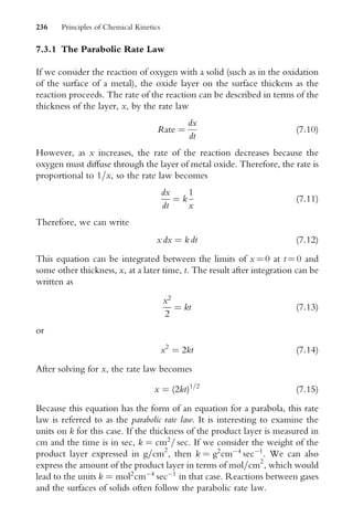


![Solving this equation for V1=3
we obtain
V1=3
¼ V1=3
o (1 a)1=3
(7:32)
Substituting for V1=3
in the rate law shown in Eq. (7.28) yields
V1=3
o V1=3
o (1 a)1=3
¼
kt
3
(7:33)
Since the initial volume of the particle, Vo, is a constant, this equation can
be written as
1 (1 a)1=3
¼ k0
t (7:34)
where k0
¼ k=3V1=3
o ¼ [4kop(3=4p)2=3
]=3V1=3
o . An equation involving
the function written as 1 (1 a)1=3
also results for other cases in which
a volume of the reacting material contracts in all three dimensions. For
example, it can be shown that a cube that is reacting on the surface also
leads to an equation of this general form, but the proof of that is left to the
reader. A rate law of this general form is frequently referred to as a contracting
volume rate law. The contracting volume model belongs to the deceleratory
class of rate laws because the reaction rate is maximum at the beginning of
the reaction when the surface area is maximum.
7.3.4 The Contracting Area Rate Law
Consider a particle of a solid that is shaped as a cylindrical rod of radius r and
length h as follows.
h
r=radius
For simplicity, we will suppose that the cylinder is very long compared to
the radius, which means that h r. Therefore, the area of the ends will be
considered to be insigniWcant compared to the area of the curved surface,
and we will assume that there is no signiWcant reaction on the ends.
Consequently, we are assuming that the length remains constant during
the reaction. Since the amount of material in the cylinder is represented by
the volume and the reaction occurs on the surface, we can write
dV
dt
¼ koS (7:35)
240 Principles of Chemical Kinetics](https://image.slidesharecdn.com/chemicalkinetics-231126172917-d2fe5718/85/CHEMICAL-KINETICS-pdf-251-320.jpg)


![Solving for V1=2
we obtain
V1=2
¼ V1=2
o (1 a)1=2
(7:50)
Substituting this value for V1=2
into Eq. (7.42), we obtain
V1=2
o V1=2
o (1 a)1=2
¼
kt
2
¼ V1=2
o [1 (1 a)1=2
] (7:51)
where k0
¼ k=2V1=2
o . Therefore, the rate law can be simpliWed to give
1 (1 a)1=2
¼
kt
2V
1=2
o
¼ k0
t (7:52)
The rate law for the contracting area shows that a plot of 1 (1 a)1=2
versus time will lead to a straight line if the reaction follows a ‘‘1=2-order’’
rate law. This is another of the deceleratory rate laws.
A few words are in order at this point concerning the apparent rate
constant. If a plot is made of 1 (1 a)1=2
versus time and a straight line is
obtained, the slope of that line will enable a calculation of k0
to be made.
If the reaction is subsequently carried out at several temperatures, an
Arrhenius plot can be made and an activation energy can be determined.
This is assuming, of course, that the rate constant follows Arrhenius
behavior, an assumption that cannot always be made for solid state reactions.
However, the rate constant k0
has incorporated in it other factors related to
the geometry of the system. For this case, k0
¼ k=2V1=2
o and k ¼ 2ko(ph)1=2
.
Therefore, because the measured rate constant is not that expressed in the
original diVerential rate law, the line that results from the Arrhenius
plot will be displaced upward or downward by a constant amount. While
this does not aVect the value of the activation energy calculated from the
slope of the line, it does aVect the intercept. Therefore, the Arrhenius
plot cannot be used directly to determine the pre-exponential factor from
the intercept.
7.4 THE PROUT–TOMPKINS EQUATION
In Chapter 2, the eVect of a product of a reaction functioning as a catalyst
was examined. It was shown that this type of behavior resulted in a
concentration versus time curve that is sigmoidal in shape. It appears that
there is autocatalysis in the early stages of some reactions in the solid state,
Kinetics of Reactions in the Solid State 243](https://image.slidesharecdn.com/chemicalkinetics-231126172917-d2fe5718/85/CHEMICAL-KINETICS-pdf-254-320.jpg)


![The Prout–Tompkins rate law describes a process that involves linear-
branching chain nuclei that can be terminated when they reach the product
phase. It is generally used to analyze the acceleratory portion of reactions
(typically up to a ¼ 0:3 or so). An equation having this form was originally
used by Prout and Tompkins in their study on the decomposition of
potassium permanganate, and it has also been applied to the decomposition
of silver oxide (Young, 1966).
7.5 RATE LAWS BASED ON NUCLEATION
Many chemical reactions in the solid state follow rate laws that are based on
the process of nucleation. The active sites have been observed microscop-
ically in some cases, and the phenomenon of nucleation is well established.
Although they will not be described in detail, several other processes have
nucleation as an integral part of at least the early stages. For example, crystal
growth has been successfully modeled by this type of rate law. Condensa-
tion of droplets is also a process that involves nucleation. Consequently,
kinetics of a wide variety of transformations obey rate laws that have some
dependence on a nucleation process.
The general form of the rate law that is used to describe nucleation
processes is known as the Avrami (or Avrami–Erofeev) rate law,
a ¼ 1 ektn
(7:69)
which can be written in logarithmic form as
[ ln (1 a)]1=n
¼ kt (7:70)
In this rate law, n is called the index of reaction, and it usually has values of
1.5, 2, 3, or 4. These rate laws are generally abbreviated as A1.5, A2, etc.
In particular, the A1.5 rate law (when n ¼ 1.5, 1=n is 2=3, so this rate law is
sometimes identiWed in that way) has been used to describe crystallization
processes in some solids. The rate laws having n ¼ 2 and n ¼ 3 are associated
with two- and three-dimensional growth of nuclei, respectively.
Nuclei may be present initially or they may grow in at certain locations
by a process that is usually considered to be Wrst-order. The derivation of
the Avrami rate law can be accomplished by several procedures (see Young,
1966), all of them rather complicated. Therefore, a detailed derivation will
not be presented nor is it needed to see the applications of this type of rate
law. In general, assumptions are made regarding the rate of change in the
246 Principles of Chemical Kinetics](https://image.slidesharecdn.com/chemicalkinetics-231126172917-d2fe5718/85/CHEMICAL-KINETICS-pdf-257-320.jpg)
![number of nuclei and the volume swept out by them as they react. When
the volume of all the nuclei is considered along with the volume change of
the nuclei as they react, it is possible to derive the equation
ln (1 a) ¼ C ekt
1 þ kt
kt
ð Þ2
2!
þ
(kt)3
3!
!
(7:71)
(where C is a constant representing a collection of constants that involves,
among otherthings, No). Thisequation isthe mostgeneralform of therandom
nucleation rate law. At longer times (represented by the decay region of the a
versus time curve), the term (kt)3
=3! dominates, so the equation reduces to
ln (1 a) ¼ C0
k0
t3
(7:72)
Taking the cube root of this equation and letting k00
¼ (C0
k0
)1=3
yields an
equation of the form
[ ln (1 a)]1=3
¼ k00
t (7:73)
which is an Avrami rate law with an index of 3 (the A3 case). This equation
shows that a plot of [ log (1 a)]1=3
versus time should be linear.
When written in exponential form, Eq. (7.72) becomes
a ¼ 1 eC0
k0
t3
It can also be shown that the early stages of the reaction sometimes follow a
rate law in which a varies as t4
. The general equation
a ¼ 1 ektn
(7:74)
can also be derived from certain geometric models that have been applied
to the decomposition of crystalline hydrates (Young, 1966).
In order to provide a practical example of the type of behavior exhibited
by a reaction that follows an Avrami–Erofeev rate law, the data presented in
Table 7.1 were derived. In performing the calculations, it was assumed that
the reaction follows an Avrami–Erofeev rate law with an index of 2 (the A2
rate law) and that k is 0:025 min1
.
Having a set of (a,t) data available, a graph was prepared to illustrate the
type of plot that can be expected when a reaction follows an Avrami–
Erofeev rate law. The result is shown in Figure 7.2, and the sigmoidal curve
is characteristic of a reaction that follows a nucleation rate law. In Chapter 2,
it was shown that a sigmoidal rate plot results from autocatalysis, but for
reactions in the solid state such plots are more likely to indicate that the
reaction is controlled by some type of nucleation process.
Kinetics of Reactions in the Solid State 247](https://image.slidesharecdn.com/chemicalkinetics-231126172917-d2fe5718/85/CHEMICAL-KINETICS-pdf-258-320.jpg)

![These reactions take place in the range of 47 to 638C and 70.5 to 868C,
respectively. Both reactions appear to follow an Avrami–Erofeev rate law
with an index of 2 over a range of a from 0.1 to 0.9 (see Ng, et al., 1978).
For a rate law having the form [ ln (1 a)]1=n
¼ kt, the most obvious
way to evaluate the constants n and k is to take the logarithm of both sides
of the equation, which yields
1
n
ln [ ln (1 a)] ¼ ln (kt) ¼ ln k þ ln t (7:77)
From this equation, we see that a plot of ln [ ln (1 a)] versus ln(t)
should give a straight line having a slope of n and an intercept of n[ln(k)]
when the correct value of n is used. In practice, it is usually preferable to
plot the function [ ln (1=(1 a))]1=n
versus time in order to test various
values of n. This is because the form involving the ln ln function is
insensitive to small changes in the data due to the nature of that function.
7.6 APPLYING RATE LAWS
The rate laws discussed up to this point involve a large number of math-
ematical forms that involve functions of (1 a). Those shown earlier and a
few others are summarized in Table 7.2. It is readily apparent that several of
the rate laws have very similar mathematical forms. Consequently, applying
these equations to data obtained from experiments on solid state reactions
may result in more than one of the equations giving about equally good Wt
to the data. It is frequently the case that it is virtually impossible to
determine with certainty which of the rate laws is correct if all one has to
go on is the data for a as a function of time obtained from a limited number
of kinetic runs. Because of the nature of solid state reactions, it is frequently
impossible to follow the reaction over several half-lives as is always recom-
mended for reactions in solution. In these cases, it is helpful to have data
from several diVerent experiments so that errors in the data (generally in the
a values, since it is often diYcult to determine the fraction of the sample
reacted accurately) do not make it impossible to identify the correct rate
law. (An example of this situation was illustrated in Section 1.3). The
characteristics described above can be illustrated by the following example.
Figure 7.3 was constructed using the data presented in the table.
Although the ‘‘correct’’ value of n is 2 in this case (the value used in
calculating the data), the data were also Wtted to rate laws having n values of
1.5 and 3. The resulting curves are also shown in Figure 7.3. Note that only
Kinetics of Reactions in the Solid State 249](https://image.slidesharecdn.com/chemicalkinetics-231126172917-d2fe5718/85/CHEMICAL-KINETICS-pdf-260-320.jpg)
![the line on the graph corresponding to n ¼ 2 is straight. Moreover, the line
resulting when n was set equal to 3 is concave downward while that resulting
when n was set equal to 1.5 is concave upward. It is a general characteristic
of plots that test Avrami–Erofeev rate laws that if n is larger than the correct
value, the line is curved and will be concave downward. Conversely, if n is
smaller than the correct value, the line will be concave upward.
Another conclusion can be illustrated by studying Figure 7.3. If only a
few data points were available and if they were subject to substantial errors,
as they frequently are for solid state reactions, it would be diYcult (if not
impossible) to determine the correct index of reaction. Also, some other
TABLE 7.2 Rate Laws for Reactions in Solids.
Description Mathematical Form
Acceleratory a-time curves
Power law a1=n
Exponential law ln a
Sigmoidal a-time curves
A1.5 Avrami–Erofeev one-dimensional growth of nuclei [ ln (1 a)]2=3
A2 Avrami–Erofeev two-dimensional growth of nuclei [ ln (1 a)]1=2
A3 Avrami–Erofeev three-dimensional growth of nuclei [ ln (1 a)]1=3
A4 Avrami–Erofeev [ ln (1 a)]1=4
B1 Prout–Tompkins ln [a=(1 a)]
Deceleratory a-time curves based on geometrical models
R1 One-dimensional contraction 1 (1 a)2=3
R2 Contracting area 1 (1 a)1=2
R3 Contracting volume 1 (1 a)1=3
Deceleratory a-time curves based on diVusion
D1 One-dimensional diVusion a2
D2 Two-dimensional diVustion (1 a) ln (1 a) þ a
D3 Three-dimensional diVusion [1 (1 a)1=3
]2
D4 Ginstling–Brounshtein [1 (2a=3)] (1 a)2=3
Deceleratory a-time curves based on reaction order
F1 First-order ln (1 a)
F2 Second-order 1=(1 a)
F3 Third-order [1=(1 a)]2
250 Principles of Chemical Kinetics](https://image.slidesharecdn.com/chemicalkinetics-231126172917-d2fe5718/85/CHEMICAL-KINETICS-pdf-261-320.jpg)
![function shown in Table 7.2 might Wt the data about equally well. In this
example, the data were calculated assuming that k ¼ 0:025 min1
and the
entire range of a values was used. If a more limited range of experimental a
values is available for use in the calculations, selection of the correct rate law
is not a trivial problem, especially when there are errors in the data due to
experimental conditions and measurements.
As was illustrated in Chapter 1, errors in the data can make it diYcult to
distinguish the correct rate laws, especially when the reaction is followed
only to 50 or 60% completion. For solid state reactions, it may be virtually
impossible to assign a unique rate law under these conditions because of the
mathematical similarity of the rate laws. The general rule for determining
the rate law for a reaction in kinetic studies is to follow the reaction over
several half-lives (see Chapter 1). However, this is almost never possible for
a solid state reaction and even if it were, the ‘‘correct’’ rate law could very
well be diVerent in diVerent stages of the reaction (see Section 7.1). Data
points in the range 0:1 a 0:9 are generally chosen to avoid any
induction period and the decay region unless these regions are speciWcally
under study. As a result of these factors, it is generally necessary to make a
rather large number of kinetic runs to try to determine a rate law that is
applicable to the reaction. This will be illustrated in the next section.
In Chapter 8, it will be shown that most of the rate laws shown in Table
7.2 can be put in the form of a composite rate law involving three exponents.
We will also describe the diYculties associated with attempts to determine
these exponents from (a,t) data. While the discussion up to this point has set
forth the basic principles of solid state reactions, their application to speciWc
0
0.5
1.0
1.5
2.0
2.5
3.0
3.5
100
80
60
40
20
0
Time, min
[ln(1
–a]
1/n n =1.5
n =3
n=2
FIGURE 7.3 Avarami–Erofeev plots of the data shown in Table 7.2.
Kinetics of Reactions in the Solid State 251](https://image.slidesharecdn.com/chemicalkinetics-231126172917-d2fe5718/85/CHEMICAL-KINETICS-pdf-262-320.jpg)
![studies has not been shown. In the next section, the results obtained from a
few case studies of reactions in solids will be considered to show how they
can be interpreted. In spite of the diYculties associated with studying
reactions in the solid state, a great deal of insight is often possible.
7.7 RESULTS OF SOME KINETIC STUDIES
In order to prevent the development of principles of solid state kinetics
from being an abstract exercise, summaries will be presented that illustrate
how kinetic results have been interpreted in speciWc cases. Although the
studies are not necessarily complete, they will show that a great deal of
information about solid state reactions can be deduced from kinetic studies
as long as the basic principles are understood and applied correctly.
7.7.1 The Deaquation–Anation of [Co(NH3)5H2O]Cl3
When aquapentamminecobalt(III) chloride and similar compounds are
heated, the water is driven oV and an anion replaces it in the coordination
sphere of the metal. Because an anion is replacing a volatile ligand, this type
of reaction is known as an anation reaction. In the case to be discussed here,
the reaction is
[Co(NH3)5H2O]Cl3(s) ! [Co(NH3)5Cl]Cl2(s) þ H2O( g) (7:78)
However, when other anions (e.g., Br
, NO
3 , or SCN
) are present, the
kinetic behavior of the reaction is altered. For example, activation energies
of 79, 105, and 139 kJ=mol have been reported for the Cl
, Br
, and
NO
3 compounds, respectively, in an early study. This behavior, sometimes
referred to as an ‘‘anion eVect,’’ has led various workers to postulate a
mechanism like that shown in Scheme I.
Scheme I
[Co(NH3)5H2O]Cl3 Ð
slow
[Co(NH3)5H2OCl]Cl2 (7:79)
[Co(NH3)5H2OCl]Cl2
!
fast
[Co(NH3)5Cl]Cl2 þ H2O (7:80)
In this mechanism, the slow step involves an anion leaving a lattice site and
entering the coordination sphere of the metal to give a seven-bonded
252 Principles of Chemical Kinetics](https://image.slidesharecdn.com/chemicalkinetics-231126172917-d2fe5718/85/CHEMICAL-KINETICS-pdf-263-320.jpg)
![transition state. Because both the [Co(NH3)5H2O]3þ
cation and the Cl
anion are involved in forming the transition state, the process has been
referred to as SN2. However, the compound already contains three chloride
ions per cation, and the formula [Co(NH3)5H2O]Cl3 contains both cation
and anions. Therefore, it is not clear what SN2 means when only the
compound [Co(NH3)5H2O]Cl3 is the reactant.
A mechanism like that just described is very unlikely on the basis of
energetics. First, a negative ion must leave an anion site in the lattice
which would form a Schottky defect (an ion missing from a lattice site),
which is a high-energy process. Second, the anion must attach to the
[Co(NH3)5H2O]3þ
cation to produce a 7-bonded transition state. Such
complexes require sacriWcing a considerable amount of energy in the form
of the crystal Weld stabilization energy. As a result of these processes, it can
be shown that the activation energy for this reaction would be much larger
than the 79 kJ=mol reported for the deaquation-anation reaction of the
chloride compound.
A more realistic approach to the mechanism of this reaction is that water
is lost from the coordination sphere of the metal and that it must occupy
interstitial positions in the crystal lattice. This process can be considered to
be the formation of a defect followed by diVusion of the volatile product
through the lattice (the defect-diVusion mechanism). DiVusion of H2O
through the lattice is favored by the cation and anion having greatly
diVering sizes because the fraction of free space increases as the diVerence
in size of the cation and anion increases. Therefore, since the cation is large,
water should escape most easily from the chloride compound. Thus, the
activation energy should vary with the size of the anion Cl
Br
I
,
and in a later study the reported activation energies are 110.5, 124.3, and
136.8 kJ=mol, respectively, for these anions.
Part of the misconception regarding the kinetics of the deaquation-
anation reaction stems from the fact that only a limited analysis of the
data was performed. To be complete, the data should be analyzed using all
of the rate laws shown in Table 7.2. A more recent study of this process by
Hamilton and House was completed in which the reaction was studied by
means of mass loss as the H2O is driven oV. Figure 7.4 shows typical rate
plots that were obtained for the process when carried out at several constant
temperatures.
When the data are presented in this way, the unmistakable sigmoidal
nature of the rate plots for dequation-anation of [Co(NH3)5H2O]Cl3
suggests that the process obeys an Avrami–Erofeev type of rate law. In
Kinetics of Reactions in the Solid State 253](https://image.slidesharecdn.com/chemicalkinetics-231126172917-d2fe5718/85/CHEMICAL-KINETICS-pdf-264-320.jpg)
![order to test the rate laws, several runs were carried out at each tem-
perature. When the data from a total of 32 reactions (involving four
temperatures) were analyzed by means of a computer technique that tests
all of the rate laws shown in Table 7.2, it was found that 26 of the runs gave
the best Wt with the A1.5 rate law, 4 gave the best Wt with the A2 rate law,
and 2 gave the best Wt with the R3 (contracting volume) rate law. Not a
single run gave the best Wt to the data with a Wrst- or second-order rate law.
An A1.5 rate law is one form of a nucleation rate law, and it has also been
shown to represent a diVusion process. The rate constants obtained when
using the A1.5 rate law,
[ ln (1 a)]2=3
¼ kt (7:81)
to represent the (a,t) data were used to prepare the Arrhenius plot shown in
Figure 7.5.
The slope of the line corresponds to an activation energy of 97 kJ=mol,
which is a somewhat diVerent value than the value of 79 kJ=mol reported
by others in the earlier studies. However, the earlier results were obtained
with assumptions about the rate law that do not appear to be valid.
This study serves to illustrate how the application of kinetic labels such as
SN1 or SN2 for reactions in solids can be misleading. Only by careful
analysis of data from a large number of runs using a wide range of rate
laws can a correct modeling of a reaction be obtained. Unfortunately, this
fact has been overlooked many times in the past by workers who have
assumed that the kinetics of reactions in the solid state and in solution
should be similar. It should be pointed out that since this initial application
0
0.1
0.2
0.3
0.4
0.5
0.6
0.7
0.8
100
40
20
0 60 80 120
Time, min
α
70⬚C
75⬚C
80⬚C
85⬚C
FIGURE 7.4 Rate plots for the dehydration-anation reaction of [Co(NH3)5H2O]Cl3.
254 Principles of Chemical Kinetics](https://image.slidesharecdn.com/chemicalkinetics-231126172917-d2fe5718/85/CHEMICAL-KINETICS-pdf-265-320.jpg)
![of the defect-diVusion mechanism, it has been shown that many other
reactions have kinetic features that are consistent with this mechanism.
7.7.2 The Deaquation-Anation of [Cr(NH3)5H2O]Br3
The deaquation-anation reaction of [Cr(NH3)5H2O]Br3,
[Cr(NH3)5H2O]Br3(s)
![Cr(NH3)5Br Br2(s) þ H2O(g) ð7:82Þ
illustrates some of the classic problems associated with the study of reactions
in the solid state (Ingram, 1995). When the (a,t) data for this reaction were
tested by Wtting the data to the rate laws shown in Table 7.2, none of the
rate laws gave an especially good Wt over a wide range of a values. The
sigmoidal shape of the curves showing a as a function of time suggested that
an Avrami type of rate law should be applicable. In this case, the (a,t) data
for each run were divided into two groups. The Wrst group consisted of data
with 0.1 a 0.5, while the second group consisted of data for which 0.5
a 0.9. In this way, an attempt was made to identify rate laws that
would be applicable to certain regions of the reaction rather than trying to
Wt a single rate law to the entire process.
Four reactions were carried out at each of the temperatures 85, 90, 95,
100, 105, and 1108C. From analysis of the data for the portion of the
reactions where a was in the range 0.1 to 0.5, 20 out of the 24 sets of data
gave the best Wt with the A2: [ ln (1 a)]1=2
rate law. On the other
hand, when a was in the range of 0.5 to 0.9, all 24 sets of (a,t) data gave
the best Wt with the D3: [1 (1 a)1=3
]2
(three-dimensional diVusion)
–6.0
–5.5
–5.0
–4.5
–4.0
–3.5
–3.0
–2.5
–2.0
2.70 2.75 2.80 2.85 2.90 2.95 3.00 3.05 3.10
103⫻1/T, 1/K
lnk
FIGURE 7.5 Arrheniusplot for thedehydration-anation reactionof [Co(NH3)5H2O]Cl3
when the Avrami–Erofeev rate law with n ¼ 1.5 is used.
Kinetics of Reactions in the Solid State 255](https://image.slidesharecdn.com/chemicalkinetics-231126172917-d2fe5718/85/CHEMICAL-KINETICS-pdf-266-320.jpg)
![rate law. In every case, the correlation coeYcient was at least 0.9999,
showing that the rate law Wt the data extremely well.
These results show that in the early part of the reaction the rate of the
reaction is controlled by the formation of nuclei that grow in two dimen-
sions (the A2 rate law). In the latter stage, the rate of the reaction is
controlled by diVusion of water through the lattice. Such results are in
accord with the defect-diVusion model that is described in Section 7.7.1.
It seems likely in this case that the early loss of water is from near the surface
of the particles as the process of nucleation occurs. The later stages of the
reaction involve the loss of water from the interior of the crystals and thus
are controlled by the rate of diVusion of water to the surface. It is particu-
larly important to note that for this reaction none of the rate laws gave
a good Wt to the data over a wide range of a values. However, the data are
very well correlated by two diVerent rate laws that apply to diVerent
portions of the reaction. This underscores the fact that in some cases no
single rate law models the entire reaction.
The kinetics and mechanism of this reaction serve to show that even a
comparatively simple-looking reaction in the solid state may exhibit pecu-
liarities that make it quite diVerent from other reactions that otherwise
appear similar. Of course, the reactions of H2 with I2 and with Cl2 that
were described in Chapter 1 show that this is by no means restricted to
reactions in solids.
7.7.3 The Dehydration of Trans-[Co(NH3)4Cl2]IO32H2O
When solid trans-[Co(NH3)4Cl2]IO32H2O is heated, it loses the water of
hydration and simultaneously isomerizes to cis-[Co(NH3)4Cl2]IO3. An
early study of this reaction indicated that it follows the rate law
ln (1 a) ¼ kt þ c (7:83)
However a later study showed that when the material was heated in thin
beds in a nitrogen atmosphere, the reaction was described by the rate law
ln (1 a) ¼ kt2
þ c (7:84)
In the same study, it was reported that the reaction followed a Wrst-order
rate law when the sample was arranged in thick beds. Also, the activation
energy was reported to vary from 58 kJ=mol when the static nitrogen
pressure was 0.1 torr to 116 kJ=mol when the nitrogen pressure was
256 Principles of Chemical Kinetics](https://image.slidesharecdn.com/chemicalkinetics-231126172917-d2fe5718/85/CHEMICAL-KINETICS-pdf-267-320.jpg)
![650 torr. In a Xowing nitrogen atmosphere, an activation energy of
57 kJ=mol was found.
A more recent study of this reaction was conducted to try to determine
some of the kinetic features. In this study, the kinetics of the reaction
involved using samples of trans-[Co(NH3)4Cl2]IO32H2O having a particle
size distribution of 57 + 15 pm (House and Eveland, 1994). The reaction
was carried out in the range of temperature from 120 to 1408C, and
the (a,t) data were analyzed by testing with all of the rate laws shown in
Table 7.2. Figure 7.6 shows the rate plots obtained when data in the range
0.1 a 0.8 were analyzed.
From the rate plots shown in Figure 7.6, it is readily apparent that the
reaction should follow a rate law that is one of the deceleratory types. This
suggests that the reaction could obey an order, diVusion-controlled, or
geometric type of rate law. Four runs were made at each temperature (120,
125, 130, 135, and 1408C), so data were available from a total of 20 runs.
When the data were Wtted to all of the rate laws shown in Table 7.2, 12 out
of the 20 data sets gave the best Wt with the second-order rate law
1
1 a
¼ kt (7:85)
The data from the other eight reactions all gave the best Wt with the third-
order rate law,
1
(1 a)2 ¼ kt (7:86)
0
0.1
0.2
0.3
0.4
0.5
0.6
0.7
0.8
0.9
10
5
0 15 20
Time, min
α
120⬚C
125⬚C
130⬚C
140⬚C 135⬚C
FIGURE 7.6 Rate plots for the dehydration of trans-[Co(NH3)4Cl2]IO32H2O.
Kinetics of Reactions in the Solid State 257](https://image.slidesharecdn.com/chemicalkinetics-231126172917-d2fe5718/85/CHEMICAL-KINETICS-pdf-268-320.jpg)


![where y is the percent reacted (percent completion). This is essentially the
same as three-dimensional diVusion, which can be easily seen when the
Jander equation is written as
1 1
y
100
1=3
2
¼ kt (7:88)
If y is the percent reacted, y=100 is the fraction reacted, a, so this equation
is analogous to the three-dimensional diVusion rate law,
[1 (1 a)1=3
]2
¼ kt (7:89)
Although causing a reaction between two solids by heating them is
a common practice, a reaction between two solids using ultrasound as the
energy source was studied by Kassel (1994). This work was carried out to
assess the feasibility using this technique as a basis for kinetic studies. One
reaction studied was
CdI2 þ Na2S
!
ultrasound
CdS þ 2 NaI (7:90)
The solids were suspended in dodecane, and the mixture was sonicated
using a pulsed source. At speciWc times, samples of the solids were separated
from the reaction mixture and analyzed to determine the amount of CdS
formed. The extent of reaction was found to vary with sonication time,
although the data showed considerable scatter. Although the results did not
represent a highly sophisticated kinetic study, they indicated that the Jander
equation represents a rate law that should be considered when a model for
a reaction between two solids is being sought.
In another experiment of this type, a 1:1 ratio of CdI2 and Na2S was
sonicated for a longer period of time at a lower power input. The results
obtained are shown in Table 7.3.
TABLE 7.3 Extent of Reaction Between CdI2 and Na2S When Sonicated at
Low Power.
Time, min % Conversion
1 100y
y
1=3
2
15 5.0 0.000287
30 9.7 0.00112
60 13.6 0.00226
120 20.7 0.00554
180 26.1 0.00920
260 Principles of Chemical Kinetics](https://image.slidesharecdn.com/chemicalkinetics-231126172917-d2fe5718/85/CHEMICAL-KINETICS-pdf-271-320.jpg)

![Brown, M. E., Dollimore, D., Galway, A. K., in Bamford, C.H., and Tipper, D.F. Eds.
(1980). Comprehensive Chemical Kinetics, Vol. 22, Elsevier, Amsterdam. An entire volume
dealing with all aspects of reactions in solids. Also covers material on techniques of data
analysis.
Garner, W. E., Ed. (1955). Chemistry of the Solid State, Academic Press, New York.
A standard reference on early work on solid state reactions.
Gomes, W. (1961). Nature (London), 192, 865. An interesting discussion on the interpret-
ation of the activation energy for a solid state reaction.
Hamilton, D. G., House, J. E. (1994). Transition Met. Chem. 19, 527. The kinetic study on
the deaquation-anation reaction of aquapentamminecobalt(III) chloride.
House, J. E. (1993). Coord. Chem. Rev. 128, 175–191. A review of anation reactions and
applications of the defect-diVusion mechanism.
House, J. E. (1980). Thermochim. Acta, 38, 59. The original description of the defect-
diVusion model of how reactions in solid coordination compounds take place.
House, J. E., Eveland, R. W. (1994). Transition Met. Chem. 19, 199. The report on the
dehydration of trans[Co(NH3)4Cl2]IO32H2O.
Ingram, B. V. (1995). M. S. Thesis, Illinois State University. A comprehensive study of the
dequation-anation reactions of aquapentamminechromium(III) complexes.
Kassel, W. S. (1994). M. S. Thesis, Illinois State University. A study of reactions between
solids induced by ultrasound.
Ng, W.-L., Ho, C.-C., Ng, S.-K. (1978). J. Inorg. Nucl. Chem. 34, 459. A study of how rate
laws can be applied to the dehydration of copper sulfate pentahydrate.
O’Brien, P. (1983). Polyhedron 2, 233. A review of racemization reactions of solid
coordination compounds and an extension of the defect-diVusion mechanism to
racemization.
Schmalzreid, H. (1981). Solid State Reactions, 2nd ed., Verlag Chemie, Weinheim.
A monograph on principles of solid state chemistry applied to many types of reac-
tions.
Young, D. A. (1966). Decomposition of Solids, Pergamon Press, Oxford. An excellent
treatment of decomposition reactions giving derivations of many rate laws.
PROBLEMS
1. Derive the rate law for the reaction of a gas on the surface of solid
particles that are cubic with edge length l. Assume that the diVusion of
the gas is inversely proportional to the thickness of the product layer.
What geometric information does the rate constant contain?
2. Suppose that a gas reacts with solid particles that are thin coin-shaped
cylinders, but that the reaction is only on the top and bottom circular
faces. Derive the rate law for this reaction assuming that the diVusion of
the gas is inversely proportional to the thickness of the product layer.
What geometric information does the rate constant contain?
262 Principles of Chemical Kinetics](https://image.slidesharecdn.com/chemicalkinetics-231126172917-d2fe5718/85/CHEMICAL-KINETICS-pdf-273-320.jpg)
![3. In deriving the parabolic rate law, it is assumed that the rate of diVusion
of the gaseous reactant is inversely proportional to the thickness of the
product layer. Assume that the diVusion of the reactant gas varies as eax
instead of 1=x where a is a constant and x is the thickness of the product
layer. Derive the rate law that would result in this case.
4. A solid, A, crystallizes in rods having a rectangular cross section. Sup-
pose that when A is heated, the reaction A(s) ! P(g) occurs only on the
ends of the rods. What would be the rate law for the reaction?
5. A solid compound X is transformed into Y when it is heated at 758C.
A sample of X that is quickly heated to 908C for a very short time (there
is no signiWcant decomposition) and then quenched to room tempera-
ture is later found to be converted to Y at a rate that is 2.5 times that
when an untreated sample of X when both are heated at 758C for a long
period of time. Explain these observations.
6. Suppose that the reaction A(s) ! B(g) þ C(s) is being studied. Provide a
brief discussion of the results and what kind of information the results
would provide from studying the eVects of each of the following on the
rate of the reaction of the f(a) vs. time curve.
(a) Annealing crystals of A
(b) Running the reaction under high vacuum
(c) Prior treatment of A with X-rays
(d) Varying the particle size of A
(e) Sintering of A as the reaction takes place
7. For the reaction A(g) þ B(s) ! C(s), the rate is controlled by the
diVusion of A(g) through the product layer. Assume that the diVusion
is inversely proportional to the thickness of the product layer raised to
some power, z. Derive the rate law for this process.
8. For the reaction
[Cr(NH3)5H2O]Cl3(s) ! [Cr(NH3)5Cl]Cl2(s) þ H2O( g)
which was carried out at 858C, the following data were obtained. It is
known that this reaction follows an Avrami type of rate law. Test these
data to determine n, the index of reaction.
Kinetics of Reactions in the Solid State 263](https://image.slidesharecdn.com/chemicalkinetics-231126172917-d2fe5718/85/CHEMICAL-KINETICS-pdf-274-320.jpg)

![diameter of 10 microns as it is when the average diameter is 30
microns, what does this tell you about the process?
13. The rate of racemization of solid l K3[Co(ox)3]2:6H2O (where ox
is oxalate, C2O4
2
) is found to increase as the pressure is increased.
The value for DVz
from one set of measurements was found to be
1:44 0:23 cm3
=mol while a second series of experiments yielded a
value of 1:80 0:28 cm3
=mol. Discuss mechanistic implications that
are consistent with the value of DVz
. For a discussion of this reaction,
see Brady, J., Dachille, F., Schmulbach, C. D. Inorg. Chem. 1963, 2,
803.
14. The loss of water from the complexes [Ru(NH3)5H2O]X3 (where
X ¼ Cl
, Br
, I
, or NO
3 ) has activation energies of 95.0, 97.9,
112, and 80.8 kJ=mol, respectively. The values for the entropy of
activation are 7.1, 5.2, 5.8, and 15.5 e.u., respectively. In light
of the kinetic parameters, discuss the mechanism of dehydration of the
complexes.
Kinetics of Reactions in the Solid State 265](https://image.slidesharecdn.com/chemicalkinetics-231126172917-d2fe5718/85/CHEMICAL-KINETICS-pdf-276-320.jpg)


![materials. Because both of these methods can readily yield data that are
suitable for kinetic analysis, their use for that purpose will be discussed in
greater detail. It should be pointed out that this is an area of intense research
activity, and the literature in this Weld has expanded enormously in recent
years. The methods that will be described brieXy here are included only to
show representative examples of the techniques used. Many others have
been published and an entire book could easily be written describing
nonisothermal kinetics methods and their areas of application. If fact,
such sources do already exist (see references at the end of this chapter). In
addition, thermoanalytical methods are especially valuable in the polymer
industry.
As mentioned earlier, a TGA experiment determines the mass of the
sample, either as temperature is held constant or as it is changed in some
programmed way. The mass is measured using a microbalance, which is
capable of determining a mass loss of 106
grams. Only a few milligrams of
sample are necessary to perform the TGA analysis. TGA is a most useful
technique when a reaction of the type
A(s)
!B(s) þ C( g) (8:2)
is being studied. In this kind of process, which is characteristic of numerous
solid state reactions, the extent of mass loss can be used to establish the
stoichiometry of the reaction. Consider a complex represented as
[M(NH3)6]X2 where M is a metal ion and X is an anion such as Cl
.
Heating a complex of this type in a TGA apparatus could produce a curve
such as that shown in Figure 8.1.
T1
T2
T3
T4
T5
T6
Temperature
α
FIGURE 8.1 A hypothetical TGA curve for the loss of six ammonia molecules in three
steps as illustrated by Eqs. (8.3) through (8.5).
Nonisothermal Methods in Kinetics 269](https://image.slidesharecdn.com/chemicalkinetics-231126172917-d2fe5718/85/CHEMICAL-KINETICS-pdf-280-320.jpg)
![When complexes such as [M(NH3)6]X2 are heated, there is usually a
stepwise loss of the volatile ligands, NH3. The three mass plateaus shown
in Figure 8.1 are indicative of the reactions. With the initial and Wnal
temperatures being indicated, these reactions could be
[M(NH3)6]X2(s)
!
T1 ! T2
M(NH3)4X2(s) þ 2NH3( g) (8:3)
M(NH3)4X2(s)
!
T3 ! T4
M(NH3)2X2(s) þ 2NH3( g) (8:4)
M(NH3)2X2(s)
!
T5 ! T6
MX2(s) þ 2NH3( g) (8:5)
Whether these are, in fact, the actual reactions must be determined by
comparing the observed mass losses with those expected for the reactions.
Frequently, it is not easy to determine the temperatures T1,T2, . . . ,
owing to the nearly horizontal nature of the curve in those regions and
the attendant indistinct beginning and ending temperatures of the reaction
steps. This means also that it is not easy to determine accurately the mass
loss in such cases. Because of this, some instruments also compute the trace
of the Wrst derivative of the mass curve simultaneously. This DTG (deriva-
tive thermogravimetric analysis) makes it much easier to determine where a
zero slope indicates that the sample is undergoing no change in mass.
Therefore, the reaction stoichiometry can be more accurately determined.
Both DSC and TGA allow the fraction of the reaction complete, a, to be
determined as a function of temperature. When the mass loss for the reaction
being studied has been determined from the plateaus of the TGA trace, the
mass loss at speciWc temperatures can be determined by comparing the mass
lost from the beginning of the reaction up to that temperature with the mass
loss for the complete reaction. If the mass loss at temperature Ti is Wi and the
mass loss for the complete reaction is Wt, then a ¼ Wi:Wt. Thus, if a certain
reaction corresponds to a mass loss of 40% and the observed mass loss at some
temperature is 10%, the value of a at that temperature is 10=40 ¼ 0.25.
In DSC, the extent of reaction is obtained by Wrst determining the total
area of the peak that corresponds to the complete reaction. The required
information from the experiment is the fraction of the complete reaction at
a series of temperatures so that nonisothermal kinetics procedures can be
applied. At a speciWc temperature, the partial peak area is determined, and
the fraction of the complete reaction at that temperature is determined by
dividing the area of the peak up to that temperature by the total peak area.
A typical endothermic peak in a DSC trace is shown in Figure 8.2. In this
case, the temperatures at which a is to be determined are indicated as
270 Principles of Chemical Kinetics](https://image.slidesharecdn.com/chemicalkinetics-231126172917-d2fe5718/85/CHEMICAL-KINETICS-pdf-281-320.jpg)

![In the case where n ¼ 1, the equation becomes
ln ln
1
1 a
2 ln T ¼ ln
AR
bEa
1
2RT
Ea
Ea
RT
(8:12)
At room temperature, 2RT is approximately 5 kJ=mol (1.2 kcal=mol), so
for most reactions EaRT. As a result, the second term inside the
parentheses is negligible, so the term
ln
AR
bEa
1
2RT
Ea
(8:13)
can normally be considered to be a constant when Wtting data to rate laws.
Therefore, the rate equations shown in Eqs. (8.11) and (8.12) can be put in
a linear form when the left-hand side is plotted against 1=T. The intercept
is ln [(AR=bEa)(1 (2RT=Ea))] and the slope is Ea=R. The frequency
factor, A, can be calculated from the intercept. It has been stated that only n
values of 1, 1=3, 2=3, 1, and 2 have any chemical basis, and examination of
the rate laws shown in Table 7.2 indicates that this is the case. Some
workers also include the value of 1=2 in the list of possible values.
The way in which the analysis is performed is to determine a series of
values for the fraction of the reaction complete, ai, at a series of temper-
atures, Ti. Then the functions represented by the left-hand side of the
equation are computed for each pair of (a,T) values for various values of n.
The values for the functions are then plotted against 1=T, and the series that
gives the most nearly linear plot is presumed to correspond to the ‘‘correct’’
reaction index, n. Table 8.1 shows values of ai and Ti for a hypothetical
reaction. Equations (8.11) and (8.12) were used to calculate the f (a,T)
values to make plots of these values versus 1=T for the diVerent trial values
of n. In keeping with the usual practice, n values of 0, 1=3, 2=3, 1, and
TABLE 8.1 Values of a and f(a) for Various Trial Values of n. When Ea¼100 kJ=mol.
T (K) 103
=T a n ¼ 0 n ¼ 1=2 n ¼ 2=3 n ¼ 1 n ¼ 2
410 2.439 0.06974 14.695 14.683 14.671 14.659 14.623
420 2.381 0.14317 14.024 13.999 13.974 13.948 13.870
430 2.326 0.27660 13.413 13.361 13.309 13.255 13.089
440 2.273 0.49189 12.883 12.781 12.674 12.564 12.206
450 2.222 0.77010 12.480 12.283 12.068 11.833 11.010
460 2.174 0.97868 12.284 11.937 11.489 11.195 8.436
Nonisothermal Methods in Kinetics 273](https://image.slidesharecdn.com/chemicalkinetics-231126172917-d2fe5718/85/CHEMICAL-KINETICS-pdf-284-320.jpg)
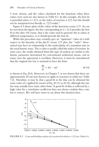
![The nonisothermal kinetic method described earlier is known as the
Coats and Redfern method (Coats and Redfern, 1964). It is only one of
many analysis methods that have been developed to analyze data from
nonisothermal kinetic studies. It is one of the most widely applied methods,
and it is one of the most straightforward procedures. The entire analysis can
be programmed for use on a microcomputer or programmable calculator.
In this case, the (a,T) data are entered only once, and the entire sequence of
n values is tested automatically. The value of n giving the best Wt is
identiWed by the correlation coeYcient by means of linear regression.
Theoretical values of n are 0, 1=3, 1=2 , 2=3, 1, and 2 because they have
some justiWcation on the basis of geometrical, contracting, or reaction order
models (see Chapter 7). Also, it is possible to treat n as simply an exponent
to be varied, and iterative procedures have been devised to identify any
value of n that provides the best Wt to the data. It is by no means clear what
an n value of 0.43 or 1.12 means in terms of a mechanism, however.
Although we have arrived at a procedure to identify a value of n, there is
no realistic way to relate that value to a mechanism.
8.3 THE REICH AND STIVALA METHOD
An interesting variation on the Coats and Redfern method has been
developed by Reich and Stivala (1980). The method makes use of an
iterative technique to arrive at the best value of n to Wt the a,T data to a
rate law. It is best employed using a computer to perform all of the
computations. The integrated rate equation is written in the form
1 (1 a)1n
(1 n)
¼ ln
ART2
bEa
1
2RT
Ea
eEa=RT
(8:15)
where the temperature integral has been written as a truncated series as
before. As before, we recognize that Ea RT so that [1 (2RT=Ea)] is
very nearly a constant. Therefore, Eq. (8.15) can be written in a two-point
form as
ln
1 (1 ai)1n
1 (1 aiþ1)1n
Tiþ1
Ti
2
#
¼
Ea
R
1
Ti
1
Tiþ1
(8:16)
This equation has a linear form when we let y represent the f (a,T) on the
left-hand side and x represent [(1=Ti) (1=Tiþ1)] on the right-hand side.
Nonisothermal Methods in Kinetics 275](https://image.slidesharecdn.com/chemicalkinetics-231126172917-d2fe5718/85/CHEMICAL-KINETICS-pdf-286-320.jpg)


![changed iteratively. Therefore, a recalculation of Ea=R using these data
when one a value is large will give a value close to the test Ea=R computed
with the Wrst two data points only when n has approximately the correct
value. For example, using a2 ¼ 0:06740 and a3 ¼ 0:98235, Ea=R varies
from about 347 for n ¼ 0.4 to 17,258 for n ¼ 2. Clearly, because the correct
value of Ea=R is about 12,000, this value will be obtained only when
n ¼ 1.67, and the calculated Ea=R is very sensitive to the n value. Using the
Wrst iterate Ea=R value, the function
F1 ¼
exp
Ea
R
1
T3
1
T2
T3
T2
(8:17)
is calculated using T2 and T3. Then the function
F2 ¼
[1 (1 a2)1n
]
[1 (1 a3)1n
]
(8:18)
is computed with no ¼ 0, and the result is compared to the value of F1. It is
easily shown that if F2 F1, then the iterated reaction index, n0
, is smaller
than the ‘‘correct’’ n (n0
n when F2 F1). The process continues by
incrementing n0
by 0.100001 (so that n0
is never exactly equal to 1) and
repeating the calculations. At the point where F1 F2, n0
is greater than n by
an amount less than 0.1 for the Wrst iterate determined for Ea=R. This Wxes an
approximate upper limit of n0
, usually within 0.1 of the ‘‘correct’’ value.
At this point, the value of n0
calculated from (a2,T2) and (a3,T3) using the Wrst
iterate Ea=R value is reduced by 0.1, and the increment to n0
is reduced from
0.1 to 0.01 as a step reWnement. The resulting n0
is used to recalculate a second
iterate Ea=R value using the Wrst two data pairs. This Ea=R value is very
nearly the correct one because the value of n0
used is correct to within 0.1.
Having a nearly exact second iterate to Ea=R, the function F1 is
calculated using points (a2,T2) and (a3,T3). Processing continues by com-
puting the function F2 iterating with Dn ¼ 0:01. When F2 F1 occurs,
the computation ends, and n0
has been determined with an upper limit of
0.01 of the ‘‘correct’’ value. If desired, the entire process can be repeated
to obtain a third iterate to Ea=R using the value of n0
, which is very close
to the correct value, and an increment of Dn ¼ 0:001. This is never
really necessary, however. The three-point method is very compact and
requires a minimum of memory in the computing machine. Therefore, it is
adaptable to programmable calculators having small capacity. Exhaustive
278 Principles of Chemical Kinetics](https://image.slidesharecdn.com/chemicalkinetics-231126172917-d2fe5718/85/CHEMICAL-KINETICS-pdf-289-320.jpg)
![calculations using simulated errors in the data have shown that this method
actually yields values of n and Ea, which are less sensitive to errors in a than
are those based on the Coats and Redfern or Reich and Stivala methods.
8.5 A METHOD BASED ON FOUR (a,T) DATA
PAIRS
Another method for determining n and Ea=R from (a,T) data makes use of
four data pairs. In this method, it is assumed that four values, a1, a2, a3,
and a4, are known at four temperatures, T1, T2, T3, and T4, respectively.
Further, for simplicity, we will assume that a1 a2 a3 a4. The
method makes use of the two-point form of the Coats and Redfern
equation, written as
ln
1 (1 a1)1n
]
[1 (1 a2)1n
]
T2
T1
2
#
1
T2
1
T1
¼
Ea
R
(8:19)
By considering an analogous equation for the points (a3,T3) and (a4,T4),
elimination of Ea=R yields
ln
1 (1 a3)1n
]
[1 (1 a4)1n
]
T4
T3
2
#
1
T4
1
T3
¼
ln
1 (1 a1)1n
]
[1 (1 a2)1n
]
T2
T1
2
#
1
T2
1
T1
(8:20)
However, the two sides of this equation will be equal only when n has the
correct value. Therefore, it is a simple matter to set up a calculation in
which the value of n is changed iteratively until the two sides of the
equation are equal using the same type of iteration on n described earlier.
A graphical method using this approach has also been described in which
the left-hand and right-hand sides of the equation are plotted as functions of
n. the point of intersection of the two curves yields the correct value of n.
The advantages of this method are similar to those described for the three-
point method. It is a compact method that can easily be programmed on a
calculator or computer. Also, it is more resistant to errors in than is either
the Coats and Redfern or Reich and Stivala methods, which are both based
on the same general rate law shown in Eq. (8.6).
Nonisothermal Methods in Kinetics 279](https://image.slidesharecdn.com/chemicalkinetics-231126172917-d2fe5718/85/CHEMICAL-KINETICS-pdf-290-320.jpg)

![Many of these methods are based on the rate law shown in Eq. (8.6),
which is not a general rate law because it can not be put in a form to
describe diVusion control or Avrami rate laws (see Chapter 7). In 1983,
Reich and Stivala removed the constraint imposed by Eq. (8.6) by devel-
oping a kinetic analysis procedure that tests most of the common types of
rate laws including Avrami, diVusion control, and others not covered
by Eq. (8.6). The method is based on a computer program that Wts the
(a,T) data to the rate laws and computes the standard error of estimate
(SEE) for each so that the rate law that provides the best Wt to the data
can be identiWed. It is still true that when data from a large number of
runs are considered, it is rare that a given rate law Wts the data from all
the runs. It is still necessary to make a large number of runs and examine
the results to determine the rate law that Wts the data from most of the
runs.
The 1983 method of Reich and Stivala is still one of the most powerful
and useful techniques for studying kinetics of solid state reactions using
nonisothermal techniques. The article describing the method also has a
listing of the computer program for implementing the procedure (Reich
and Stivala, 1983). In general, this method gives excellent agreement with
the results obtained from other studies where data from nonisothermal
experiments are Wtted to the rate laws shown in Table 7.2. In addition to
the methods discussed here and in Section 8.3, Reich and Stivala have
described a rather large number of data analysis procedures for use in
analyzing data from nonisothermal analytical techniques.
8.8 THE GENERAL RATE LAW AND
A COMPREHENSIVE METHOD
When the rate laws shown in Table 7.2 are examined, it is found that
(1 a), ln (1 a), and a occur in various combinations to comprise
the rate laws. Moreover, in some of the rate laws, these expressions are
raised to some power. Therefore, a general rate law that describes almost
any reaction taking place in the solid state can be written to include
all of these features. That rate law is for a nonisothermal reaction and is
written as
da
dT
¼
A
b
am
(1 a)n
[ ln (1 a)]p
eEa=RT
(8:26)
Nonisothermal Methods in Kinetics 281](https://image.slidesharecdn.com/chemicalkinetics-231126172917-d2fe5718/85/CHEMICAL-KINETICS-pdf-292-320.jpg)
![where b is the heating rate and the other symbols have their usual meanings.
If the natural logarithm is taken of both sides of the equation, the result is
ln
da
dT
¼ ln
A
b
þ m ln a þ n ln (1 a) þ p[ ln (1 a)]
Ea
RT
(8:27)
In this equation, m, n, and p as well as Ea and A are unknowns for a
particular reaction. This suggests that if a and da=dT were known at Wve
temperatures, a system of Wve equations containing Wve unknowns could be
solved to Wnd m, n, p, A, and Ea. Of course it would be preferable to have
an over-determined system by having many a and (da=dT) data pairs.
Then multiple linear regression could be employed to determine the
appropriate values for the Wve unknown quantities. Such a procedure
would enable one to identify any of the rate laws shown in Table 7.2 by
determining the appropriate exponents, m, n, and p. For example, if m and
p are both zero and n ¼ 2, a second-order process is indicated. If m and n are
both zero and p ¼ 1
/2 , an Avarami A2 rate law is indicated. By varying the
exponents appropriately, all of the rate laws shown in Table 7.2 can be
reduced to special cases of the general rate law shown in Eq. (8.27).
In Chapter 7, it was shown that in the analysis of the (a,T) data to
determine the best-Wtting rate law that the same rate law was not necessarily
indicated as Wtting all runs, and that numerous runs might be required to
obtain a consensus. An elaborate computer program has been developed to
solve the system of equations using a numerical technique known as
Gauss–Jordan condensation with pivotal rotation (Lowery, 1986). To test
the procedure, data known to Wt speciWc rate laws were needed. These data
were obtained by solving the general rate law shown in Eq. (8.27) numer-
ically using a fourth-order Runge–Kutta technique. In performing the
calculations, solutions were carried out with various combinations of ex-
ponents, m, n, and p (e.g., m ¼ 0, n ¼ 1=3, and p ¼ 0; m ¼ 1=3, n ¼ 0, and
p ¼ 0; m ¼ 0, n ¼ 1=3, and p ¼ 1=3, etc.). This was done so that the (a,T)
from a variety of rate laws could be tested. Also, the general analysis
procedure was designed so that the test data could be analyzed not only
with a procedure that would determine three exponents, but also one that
would keep some of the exponents at zero and ‘‘force’’ the Wtting of the
data to special case rate laws in which only the other exponents would be
allowed to vary. For example, if m ¼ p ¼ 0 and only n can vary, the data are
forced to Wt a rate law having the form
da
dT
¼
A
b
(1 a)n
eEa=RT
(8:28)
282 Principles of Chemical Kinetics](https://image.slidesharecdn.com/chemicalkinetics-231126172917-d2fe5718/85/CHEMICAL-KINETICS-pdf-293-320.jpg)
![If m ¼ n ¼ 0 and only p is allowed to vary, the data are forced to Wt a rate
law having the form
da
dT
¼
A
b
[ ln (1 a)]p
eEa=RT
(8:29)
which is the form of the Avrami rate laws. Obviously, if the (a,T) data
were calculated using n ¼ 1=3 and m ¼ p ¼ 0, and then the (a,T) data
analyzed using a method that forced them to Wt a rate law in which only
p could vary, some ‘‘interesting’’ results should be obtained. In order to
provide a comparison with other methods, the (a,T) data were also ana-
lyzed using the Coats and Redfern method (Eq. (8.11)), and the Reich and
Stivala method (Eq. (8.15)) which is based on the same rate law as the Coats
and Redfern method.
How well the procedure works is illustrated by the following cases.
Table 8.3 shows the results obtained by applying the general procedure
to (a,T) data, which were derived from a rate law that is of the form
involving a single exponent, m ¼ 0.333. In calculating the values used in
this case, n ¼ p ¼ 0 was assumed. The results shown in the table clearly
indicate that any time the general procedure allowed for m to be one of the
exponents to be determined, the Wt was very good. However, if the
procedure used was one in which m was omitted from the computation
(n, p, or np type of rate law), the Wt was quite poor, as expected. Finally,
when the computational procedure used a rate law of the mnp type (all
TABLE 8.3 Results Obtained from the Analysis of Data Derived Using an am
Type of Rate Law with Data for Which m ¼ 0.333 and Ea¼100 kJ=mol.
Typea
Calculated
Ea(kJ=mol) m n p Sb
m 100.2 0.332 0.000 0,000 0:36 109
n 152.9 0.000 0.003 0.000 0:48 109
p 151.7 0.000 0.000 0.008 0:42 109
mn 100.1 0.333 0.000 0.000 0:36 109
np 136.5 0.000 0.042 0.102 0:24 109
mnp 97.9 0.354 0.003 0.007 0:24 109
a
The rate law type refers to the exponents treated as variables and allowed to vary in the data
analysis procedure to analyze the (a,T) data.
b
S is the sum of squares of errors from regression Wtting of the data to the rate laws.
Nonisothermal Methods in Kinetics 283](https://image.slidesharecdn.com/chemicalkinetics-231126172917-d2fe5718/85/CHEMICAL-KINETICS-pdf-294-320.jpg)
![three exponents treated as variables to be determined), the Wt was accept-
able. In the numerical solution of the diVerential equation to obtain the
(a,T) data, Ea ¼ 100 kJ= was used and that value was successfully deter-
mined by the computations using any of the rate laws that tested an
‘‘m-type’’ rate law. Similar results are shown in Tables 8.4 and 8.5 for
rate laws of the ‘‘n-type’’ and the ‘‘p-type.’’ In each case, the general
procedure in which m, n, and p were all determined or any abbreviated
TABLE 8.4 Results Obtained from the Analysis of Data Derived Using an
(1 a)n
Type of Rate Law with Data for Which n ¼ 0.333.
Typea
Calculated
Ea(kJ=mol) m n p Sb
m 237.1 3.186 0.000 0,000 0:26 102
n 100.0 0.000 0.333 0.000 0:84 109
p 227.5 0.000 0.000 1.18 0:26 103
mn 100.0 0.000 0.333 0.000 0:84 109
np 100.0 0.000 0.333 0.000 0:84 101
mnp 101.2 0.005 0.332 0.006 0:77 109
a
The rate law type refers to the exponents treated as variables and allowed to vary in the data
analysis procedure to analyze the (a,T) data.
b
S is the sum of squares of errors from regression Wtting of the data to the rate laws.
TABLE 8.5 Results Obtained from the Analysis of Data Derived Using a
[ ln (1 a]p
Type of Rate Law with Data for Which p ¼ 0.333 (Avrami, A3).
Typea
Calculated
Ea(kJ=mol) m n p Sb
m 187.7 3.219 0.000 0,000 0:11 103
n 73.8 0.000 0.121 0.000 0:51 104
p 100.0 0.000 0.000 0.333 0:46 108
mn 31.1 1.311 0.072 0.000 0:25 105
np 99.9 0.000 0.000 0.333 0:44 108
mnp 97.9 0.021 0.001 0.328 0:38 108
a
The rate law type refers to the exponents treated as variables and allowed to vary in the data
analysis procedure to analyze the (a,T) data.
b
S is the sum of squares of errors from regression Wtting of the data to the rate laws.
284 Principles of Chemical Kinetics](https://image.slidesharecdn.com/chemicalkinetics-231126172917-d2fe5718/85/CHEMICAL-KINETICS-pdf-295-320.jpg)
![procedure that contained the appropriate rate law exponent successfully
analyzed the data to reproduce the values of rate Ea, A, and the exponents.
For the same calculated a, T, and da=dT data that gave the results
shown in Table 8.3 when analyzed by the comprehensive method, the
Coats and Redfern method gave an n value of approximately zero, an
activation energy of 152 kJ=mol, and a correlation coeYcient of 1.000!
The reason for these totally Wctitious results is that the rate law
da
dT
¼
A
b
(1 a)n
eEa=RT
(8:30)
cannot be put in a form that represents a rate law based on am
, the actual
rate law to generate the a and da=dT data. However, the data may be Wt by
the Coats and Redfern equation with some value of n even if the rate law is
of the wrong form.
Table 8.4 shows the results obtained when the rate law used to deter-
mine the (a,T) data was of the ‘‘n-type’’ and those data were analyzed using
the complete procedure and procedures that involve incomplete forms. To
obtain a, T, and da=dT data that were analyzed to give the results shown in
Table 8.4, the rate law
da
dT
¼
A
b
(1 a)1=3
eEa=RT
(8:31)
was solved numerically. This rate law is of exactly the same form as that
used in the Coats and Redfern analysis, so that method would be expected
to return the input values for n and Ea. The actual results obtained were
n ¼ 0.33 and Ea ¼ 99:7 kJ=. In this case, either the robust calculation to
determine m, n, and p or the method of Coats and Redfern will yield
equally reliable results.
In Table 8.5, the results obtained using a, T, and da=dT data that Wt an
Avrami type of rate law are shown. The general method can, of course, be
used to Wt rate laws containing any combination of m, n, and p exponents.
Clearly, any of the procedures testing a rate law containing the exponent p
work well. When analysis of the same da=dT data by the method of Coats
and Redfern is attempted, the results are n ¼ 0.125 and Ea ¼ 72:9 kJ=.
There is not agreement between these results and the input data used in
solving the rate equation numerically, because the Coats and Redfern
method is based on an equation that cannot represent a rate law of
the A3 Avrami type, which is based on [ ln (1 a)]1=3
as the function
of a.
Nonisothermal Methods in Kinetics 285](https://image.slidesharecdn.com/chemicalkinetics-231126172917-d2fe5718/85/CHEMICAL-KINETICS-pdf-296-320.jpg)


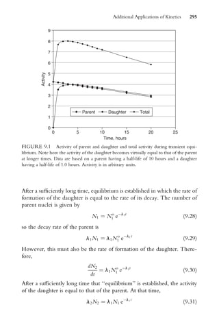


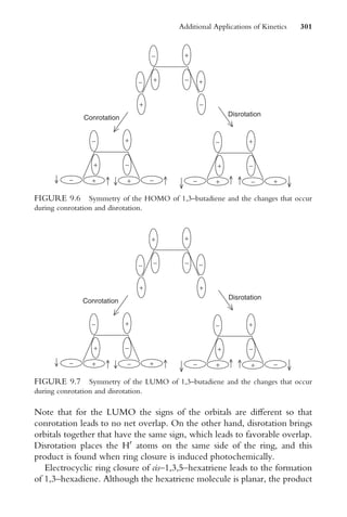
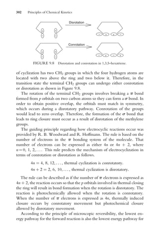

![scales’’ that have been devised, but only a few of the more common ones
will be described. Some are based on dipole moment, dielectric constant, or
other properties of the solvent molecules. In view of this vast body of
literature and the importance of the topic, it is appropriate to describe
brieXy a few of the approaches that have been taken.
From the outset, it should be recognized that a solvent produces eVects
on both the activation energy and the activation entropy. The equilibrium
that leads to the formation of the transition state is governed by the
relationship
DGz
¼ DHz
T DSz
¼ RT ln Kz
(9:37)
with the rate constant being determined by the concentration of the
transition state, which is determined by the magnitude of Kz
. Figure 9.9
shows a general indication of the eVect produced by two solvents, S1 and
S2, on the activation energy.
The eVect of the solvent on the rate of a reaction is the result of lowering
the free energy of formation of the transition state by changing the en-
thalpy, entropy, or both. This could also result from changing the state of
the reactants, because it is the diVerence between the free energies of the
reactants and the transition state that determines DGz
. For this discussion,
Reaction coordinate
Energy
Products
Reactants
Ea(S1)
∆E
[ ]+
+
Ea(S2)
FIGURE 9.9 ProWles for a reaction carried out in two solvents. The activation energies
for the reaction in the two solvents are Ea(S1) and Ea(S2), with solvent 2 being one that
enhances the formation of the transition state.
304 Principles of Chemical Kinetics](https://image.slidesharecdn.com/chemicalkinetics-231126172917-d2fe5718/85/CHEMICAL-KINETICS-pdf-315-320.jpg)


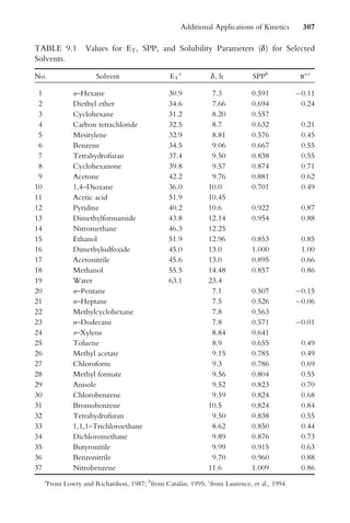


![Catalysis (continued )
gas phase reactions and, 145–147, 145f
hydrogenation reactions and, 28–30, 29f
Langmuir adsorption isotherm and,
145, 145f
Chain mechanisms. See Free-radical
mechanisms
Charge neutralization=dispersion, 167–168
Chemical kinetics, 1–2, 20
Chlorobenzene=amide ion reaction
kinetic isotope effect and, 105–106
tracer method and, 101–102
Christiansen, 132
CNDO. See Complete neglect of
differential overlap approach
Coats Redfern method
caution regarding, 286
four (a,T) data pairs method and, 279
Gauss-Jordan condensation technique
and, 283, 285–286
heating rate regarding, 272
kinetic analysis via, 271–274, 273t, 274f
practicality of, 275
Reich Stivala method regarding,
275–276
TGA and, 271
three (a,T) data pairs method and,
276, 279
Coenzymes, 206
Cofactors, 206
Cohesion energies
density and, 172–174
ideal solutions and, 172–175
solubility parameter and, 159–163
solvent and, 175–176
thermodynamics and, 174–175
Collision complex, 177
Collision theory
activation energy and, 114–115, 114f
collision frequency calculation in,
111–114, 112f
collision frequency model and, 112f
collisional cross section and,
112–113, 112f
experimental rates compared to,
115–116
gas phase reactions and, 111–116,
112f, 114f
problems with, 119
reaction rate description in, 111–112
reaction requirements and, 111, 115–116
steric factor and, 116, 119
temperature and, 115
Compensation effect, 189–191, 190f
Competitive inhibition, 216–218, 218f
Complete neglect of differential overlap
(CNDO) approach, 138
Concentration
autocatalysis and, 65f, 67–68, 69f
first-order rate law and, 5–8, 6f, 8f
half-life and, 7–8, 8f, 10, 11–12, 13
Nth-order rate law and, 13
rate dependence on, 4–13
reaction rates and, 2–3, 3f
second-order rate law and, 8–10, 9f
solid state regarding, 231–232
zero-order rate law and, 10–12, 12f
Consecutive reactions. See Series reactions,
first-order; Series reactions, two
intermediate
Continuous-flow system, 94–95, 94f
Contracting area rate law, 240–243
Contracting sphere rate law, 238–240
Contracting volume rate law, 240
Covalent bonding, 311–313
Cracking, 29–30
Critical configuration, 20–21
D
Data analysis, 2, 13–15, 14f, 15f, 251
Deaquation-anation
of [Co(NH3)5H2O]Cl3, 252–255,
254f, 255f
of [Cr(NH3)5H2O]Br3, 255–256
Debye, Peter, 154
Debye-Hückel limiting law, 182, 183–184
Decarboxylation of lactones, 196–198, 197f
Decay constant, 289
Decay region, 232f, 233
Deceleratory rate, 238, 239, 243
Defect-diffusion mechanism, 253–255, 256
Dehydration of trans-
[Co(NG3)4Cl2]IO3 2H2O,
256–259, 257f
Derivative thermogravimetric analysis
(DTG), 270
Dielectric constant, 305–306
Differential method, 280
Differential scanning calorimetry
(DSC), 267
applications=research using, 268–269
enthalpy and, 268
fraction of the sample and, 270–271, 271f
nonisothermal methods and, 267–269,
270–271, 271f
Dipole moment, 154, 168, 305
Dipole-dipole association, 167
Dipole-induced dipole forces, 156, 163
318 Index](https://image.slidesharecdn.com/chemicalkinetics-231126172917-d2fe5718/85/CHEMICAL-KINETICS-pdf-329-320.jpg)


![Reforming, 30
Reich Stivala
four (a,T) data pairs method and, 279
Gauss-Jordan condensation technique
and, 283
iterative method of, 275–276
1983 method of, 280–281
three (a,T) data pairs method and,
276, 279
Relaxation techniques
fast reactions and, 95–96
kinetic analysis of, 97–98
stress and, 96
time and, 98
types of, 96–97
Retention, 233–234
Reversible reactions
first-order, 58–64, 62f, 62t, 63f
hypothetical reaction illustrating, 61–64,
62f, 62t, 63f
initial part of, 62–64, 63f
possible cases of, 64
Rice, O. K., 129
Roberts, J. D., 101
RRK theory, 129–130
RRKM theory, 130–131
Runge-Kutta, fourth order, method,
276–277, 277t
S
SCF. See Self-consistent field approach
Schmid, R., 74, 75
Scott, R., 198, 199
Secondary isotope effects, 107
Second-order mixed case reaction
balancing coefficients and, 40–41
ethyl acetate hydrolysis and, 41–42, 42t,
43f
mathematics concerning, 37–41
Second-order rate law, 3, 8–10, 9f, 10
Secular equilibrium, 294–296, 296f
SEE. See Standard error of estimate
Self-consistent field (SCF) approach, 138
Series reactions, first-order
case examples for, 50–53, 50f, 51f
equations for, 48–50, 51–53
intermediate in, 47
steady-state=stationary state
approximation and, 52
time and, 52–53
unlikely case regarding, 50, 50f
Series reactions, two intermediate
sequential, 56–58, 58f
simultaneous, 53–56, 55f, 58
species relationship in, 57–58, 58f
time and, 55–56, 57
Shock tube method, 96
Significant structure theory, 153
Sintering, 29, 233–234
Solids. See also Adsorption
activation energy regarding, 230, 231
Coats Redfern method and, 271–275,
273t, 274f
concentration and, 231–232
contracting area rate law and, 240–243
contracting sphere rate law and, 238–240
contracting volume rate law and, 240
deaquation-anation studies on, 252–256,
254f, 255f
decay region and, 232f, 233
deduction of information and, 229
defect-diffusion mechanism and,
253–255, 256
dehydration of trans-
[Co(NG3)4Cl2]IO3 2H2O and,
256–259, 257f
differential method regarding, 280
diffusion and, 231–232
DSC and, 267–269, 270–271, 271f
factors to consider regarding, 234–235
first-order rate law and, 237–238
four (a,T) data pairs method and, 279
fraction of the sample approach and,
232, 232f, 233
gas=solution reactions compared with,
229–230, 234
Gauss-Jordan condensation technique
and, 282–287, 283t, 284t
general considerations regarding,
229–234, 232f
geometrical models and, 238–243
HSIP and, 259
induction period and, 232f, 233
kinetic study results on, 252–256, 254f,
255f
mass loss=maximum rate and, 232f, 233
nucleation and, 246–249, 248f, 248t
parabolic rate law and, 236
Prout-Tompkins equation and, 243–246
random nucleation rate law and, 247
rate constant and, 243
rate law, general, and, 281–287,
283t, 284t
rate law table for, 250t
rate laws and, 235–243, 249–251, 251f
Reich Stivala methods regarding,
275–276, 280–281
retention=sintering and, 233–234
324 Index](https://image.slidesharecdn.com/chemicalkinetics-231126172917-d2fe5718/85/CHEMICAL-KINETICS-pdf-335-320.jpg)

![Temperature (continued )
doubling rate and, 69–71, 70f, 71f
DSC and, 267–269, 270–271, 271f
effect of, 16–20, 69–74
enzymes and, 17, 17f, 207, 207f
frequency factor and, 72
heating rate regarding, 272
ideal solutions and, 171
intermolecular forces and, 155, 156, 158
isokinetic, 190
jump, 96
narrow v. wide range of, 69
pressure and, 89, 92
rate constant and, 17, 17f
reaction rate relationship with, 71–74, 73f
solids and, 235
TGA and, 267–271, 269f
thermal dilatometry and, 267
vapor pressure and, 162
Termination steps, 23
TGA. See Thermogravimetric analysis
Thermal dilatometry, 267
Thermodynamics
cohesion energies and, 174–175
ideal solutions and, 169–172, 172f,
174–175
low energy pathway and, 1
pressure and, 89, 90, 91
Thermogravimetric analysis (TGA), 267
applications=research using, 268–269
Coats Redfern and, 271
dehydration of trans-
[Co(NG3)4Cl2]IO3 2H2O and, 258
DTG and, 270
mass and, 268, 269–270, 269f
nonisothermal methods and,
267–270, 269f
Third order reactions, 43–44
Three (a,T) data pairs method,
276–279, 277t
T-jump, 96
Topochemistry, 234
Tracer methods
chlorobenzene=amide ion reaction and,
101–102
examples of, 98–102
group transfer in, 100
hydrolysis of ethyl acetate and, 98–99
insertion reaction and, 99–100
Transient equilibrium, 293–294, 295f
Transient period, 94
Transition state, 16–17, 16f
Transition state theory
decomposition frequency and, 120–122
equilibrium and, 120
essential feature of, 119–120
Eyring and, 119
statistical mechanics procedure and,
122–123
transition state concentration in, 119–121
variational, 123–124
Transmission coefficient, 106
Transparency, 106
Triatomic transition state, 117, 118
Tunneling, 106, 118
Two reacting solids, 259–261, 260t, 261f
2=3-order rate law, 239
U
Ultrasound, 259–261, 260t, 261f
Uncompetitive inhibition, 219–220, 220f
Unimolecular decomposition of gases
Hinshelwood and, 129
Lindemann and, 124–129
non-reactant gas and, 126–128
ozone and, 128–129
RRK theory and, 129–130
RRKM theory and, 130–131
translational energy and, 124–126
V
Van Laar equation, 174
Variational transition state theory,
123–124
Volume of activation, 90–92
W
Water flow analogy, 3–4
Weissberger, A., 79
White, M. G., 138, 143, 148
Woodward, R. B., 302
Y
Young, D. A., 244, 246, 247, 262
Z
Zero-order rate law, 10–12, 12f
Zero-point vibrational energy, 103, 104
326 Index](https://image.slidesharecdn.com/chemicalkinetics-231126172917-d2fe5718/85/CHEMICAL-KINETICS-pdf-337-320.jpg)