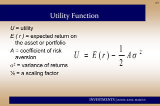
INVESTMENTS | BODIE, KANE, MARCUS
Copyright © 2011 by The McGraw-Hill Companies, Inc. All rights reserved.
McGraw-Hill/Irwin
CHAPTER 6
Prepared By
Dr. Mohammad Bayezid Ali
Professor and Adjunct Faculty
School of Business
Independent University, Bangladesh
Risk Aversion and Capital
Allocation to Risky Assets
INVESTMENTS | BODIE, KANE, MARCUS
6-2
Allocation to Risky Assets
• The process of constructing an investor portfolio can be
viewed as a sequence of two steps:
i. Deciding how much to invest in that risky portfolio versus a
safe assets such as short term t-bills.
ii. Selecting the composition of the portfolio of risky assets such
as stocks and long-term bonds.
• Investors will avoid risk unless there is a reward.
• The utility model gives the optimal allocation between a
risky portfolio and a risk-free asset.
INVESTMENTS | BODIE, KANE, MARCUS
6-3
Risk Aversion and Utility Values
• Investors are willing to consider:
– risk-free assets
– speculative positions with positive risk premiums
• Portfolio attractiveness increases with expected return
and decreases with risk.
• What happens when return increases with risk?
INVESTMENTS | BODIE, KANE, MARCUS
6-4
Table 6.1 Available Risky Portfolios (Risk-
free Rate = 5%)
Each portfolio receives a utility score to
assess the investor’s risk/return trade off
INVESTMENTS | BODIE, KANE, MARCUS
6-5
Utility Function
U = utility
E ( r ) = expected return on
the asset or portfolio
A = coefficient of risk
aversion
s2 = variance of returns
½ = a scaling factor
2
1
( )
2
U E r As
= −
INVESTMENTS | BODIE, KANE, MARCUS
6-6
Table 6.2 Utility Scores of Alternative Portfolios for
Investors with Varying Degree of Risk Aversion
INVESTMENTS | BODIE, KANE, MARCUS
6-7
An Example
A portfolio has an expected rate of return of 20% and
standard deviation of 20%. Treasury bills offer a sure
rate of return of 7%. Which investment alternative will
be chosen by an investor whose degree of risk
aversion is 4? What if it is 8?
INVESTMENTS | BODIE, KANE, MARCUS
6-8
Some Comments on Utility Value
✓ Utility value can be used to compare the rate of return
offered on risk-free investment and portfolio of risky
investment.
✓ An investor can interpret a portfolio’s utility value as
certainty equivalent rate of the portfolio.
✓ A portfolio is desirable only when its certainty equivalent
return ( i.e. utility value) exceeds that of the risk-free
alternative.
INVESTMENTS | BODIE, KANE, MARCUS
6-9
✓ A risk averse investor (i.e. A>0) prefer to invest in portfolio
of risky investment when the certainty equivalent return is
more than the return from risk-free investment.
✓ A risk neutral investor (i.e. A=0) judge risky investment
solely by their expected rate of return. The level of risk is
irrelevant to the risk-neutral investor. For this investor a
portfolio’s certainty equivalent rate is simply its expected
rate of return.
✓ A risk lover investor (i.e. A<0) is willing to engage in fair
games or gambles. This investor adjusts the expected
return upward to take into account the ‘fun’ of confronting
the investment risk.
Some Comments on Utility Value
INVESTMENTS | BODIE, KANE, MARCUS
6-10
Basic Asset Allocation
Total Market Value $300,000
Risk-free money market fund $90,000
Equities $113,400
Bonds (long-term) $96,600
Total risk assets $210,000
54
.
0
000
,
210
$
400
,
113
$
=
=
E
W 46
.
0
00
,
210
$
600
,
96
$
=
=
B
W
INVESTMENTS | BODIE, KANE, MARCUS
6-11
Basic Asset Allocation
• Let y = weight of the risky portfolio, P, is the complete
portfolio; (1-y) = weight of risk-free assets:
7
.
0
000
,
300
$
000
,
210
$
=
=
y 3
.
0
000
,
300
$
000
,
90
$
1 =
=
− y
378
.
000
,
300
$
400
,
113
$
: =
E 322
.
000
,
300
$
600
,
96
$
: =
B
INVESTMENTS | BODIE, KANE, MARCUS
6-12
• It’s possible to create a complete portfolio by splitting
investment funds between safe and risky assets.
–Let y=portion allocated to the risky portfolio, P
–(1-y)=portion to be invested in risk-free asset, F.
Portfolios of One Risky Asset and a Risk-Free
Asset
INVESTMENTS | BODIE, KANE, MARCUS
6-13
rf = 7% srf = 0%
E(rp) = 15% sp = 22%
y = % in p (1-y) = % in rf
Example Using Chapter 6.4 Numbers
INVESTMENTS | BODIE, KANE, MARCUS
6-14
Example (Ctd.)
The expected return
on the complete
portfolio is the risk-
free rate plus the
weight of P times the
risk premium of P ( ) ( )
c f P f
E r r y E r r
 
= + −
 
( ) ( )
7
15
7 −
+
= y
r
E c
By rearrangement, we get:
INVESTMENTS | BODIE, KANE, MARCUS
6-15
Example (Ctd.)
• The risk of the complete portfolio is the weight
of P times the risk of P:
y
y P
C 22
=
= s
s
INVESTMENTS | BODIE, KANE, MARCUS
6-16
Example (Ctd.)
• Again, risk of complete portfolio is
• Rearrange and substitute y=sC/sP:
( ) ( )
  C
f
P
P
C
f
C r
r
E
r
r
E s
s
s
22
8
7 +
=
−
+
=
( )
22
8
=
−
=
P
f
P r
r
E
Slope
s
P
C ys
s =
INVESTMENTS | BODIE, KANE, MARCUS
6-17
Figure 6.4 The Investment Opportunity Set
INVESTMENTS | BODIE, KANE, MARCUS
6-18
An Example
Consider the following data
Requirements:
Calculate the expected rate of return and risk of the portfolio and reward to
variability ratio (slope of the CAL Sharp Ratio) based on the following
cases:
Case 1: 85 percent investment made on T-bill.
Case 2: 65 percent investment made on T-bill.
Case 3: 25 percent investment made on T-bill.
Case 4: 10 percent investment made on T-bill.
Return Risk
T-bill 7% 0%
Risky portfolio 15% 22%
INVESTMENTS | BODIE, KANE, MARCUS
6-19
6-19
• What about points on the line to the right of the
portfolio P in the investment opportunity set?
• Suppose the investor borrows an additional
$120,000, investing the total available funds in the
risky asset. This is a leveraged position in the
risky asset, it is financed in part by borrowing.
Capital Allocation Line with Leverage
INVESTMENTS | BODIE, KANE, MARCUS
6-20
If, lend at rf=7% and borrow at rf=7%
y=(420,000/300,000)=1.4
And (1-y)=(1-1.4)=-0.4, reflects a short position in the risk-free
asset, which is borrowing position. Then:
= 7%+(1.4*8)= 18.2%
Lending range slope = 8/22 = 0.36
Borrowing range slope = 8/22 = 0.36
CAL extends to the right of point P
Capital Allocation Line with Leverage
( ) ( )
c f P f
E r r y E r r
 
= + −
 
%
8
.
30
22
*
4
.
1 =
=
= P
C ys
s
INVESTMENTS | BODIE, KANE, MARCUS
6-21
• Lend at rf=7% and borrow at rf=9%
– Lending range slope = 8/22 = 0.36
– Borrowing range slope = 6/22 = 0.27
• CAL kinks at P
Capital Allocation Line with Leverage
INVESTMENTS | BODIE, KANE, MARCUS
6-22
Figure 6.5 The Opportunity Set with
Differential Borrowing and Lending Rates
INVESTMENTS | BODIE, KANE, MARCUS
6-23
Risk Tolerance and Asset Allocation
• The investor confronting the CAL must choose one optimal
portfolio, C, from the set of feasible choices.
• Individual investor differences in risk aversion imply that, given
an identical opportunity set, different investor will choose
different positions in the risky asset. In particular, the more risk
averse investors will choose to hold less of risky asset and more
of the risk free asset.
– Expected return of the complete portfolio:
– Variance:
( ) ( )
c f P f
E r r y E r r
 
= + −
 
2 2 2
C P
y
s s
=
INVESTMENTS | BODIE, KANE, MARCUS
6-24
INVESTMENTS | BODIE, KANE, MARCUS
6-25
Table 6.4 Utility Levels for Various Positions in Risky
Assets (y) for an Investor with Risk Aversion A = 4
INVESTMENTS | BODIE, KANE, MARCUS
6-26
Optimal Allocation to Risky Portfolio for Attaining the
Highest Possible Utility
INVESTMENTS | BODIE, KANE, MARCUS
6-27
Figure 6.6 Utility as a Function of
Allocation to the Risky Asset, y
INVESTMENTS | BODIE, KANE, MARCUS
6-28
Figure 6.8 Finding the Optimal Complete
Portfolio Using Indifference Curves

chapter 6 .pdf

  • 1.
    INVESTMENTS | BODIE,KANE, MARCUS Copyright © 2011 by The McGraw-Hill Companies, Inc. All rights reserved. McGraw-Hill/Irwin CHAPTER 6 Prepared By Dr. Mohammad Bayezid Ali Professor and Adjunct Faculty School of Business Independent University, Bangladesh Risk Aversion and Capital Allocation to Risky Assets
  • 2.
    INVESTMENTS | BODIE,KANE, MARCUS 6-2 Allocation to Risky Assets • The process of constructing an investor portfolio can be viewed as a sequence of two steps: i. Deciding how much to invest in that risky portfolio versus a safe assets such as short term t-bills. ii. Selecting the composition of the portfolio of risky assets such as stocks and long-term bonds. • Investors will avoid risk unless there is a reward. • The utility model gives the optimal allocation between a risky portfolio and a risk-free asset.
  • 3.
    INVESTMENTS | BODIE,KANE, MARCUS 6-3 Risk Aversion and Utility Values • Investors are willing to consider: – risk-free assets – speculative positions with positive risk premiums • Portfolio attractiveness increases with expected return and decreases with risk. • What happens when return increases with risk?
  • 4.
    INVESTMENTS | BODIE,KANE, MARCUS 6-4 Table 6.1 Available Risky Portfolios (Risk- free Rate = 5%) Each portfolio receives a utility score to assess the investor’s risk/return trade off
  • 5.
    INVESTMENTS | BODIE,KANE, MARCUS 6-5 Utility Function U = utility E ( r ) = expected return on the asset or portfolio A = coefficient of risk aversion s2 = variance of returns ½ = a scaling factor 2 1 ( ) 2 U E r As = −
  • 6.
    INVESTMENTS | BODIE,KANE, MARCUS 6-6 Table 6.2 Utility Scores of Alternative Portfolios for Investors with Varying Degree of Risk Aversion
  • 7.
    INVESTMENTS | BODIE,KANE, MARCUS 6-7 An Example A portfolio has an expected rate of return of 20% and standard deviation of 20%. Treasury bills offer a sure rate of return of 7%. Which investment alternative will be chosen by an investor whose degree of risk aversion is 4? What if it is 8?
  • 8.
    INVESTMENTS | BODIE,KANE, MARCUS 6-8 Some Comments on Utility Value ✓ Utility value can be used to compare the rate of return offered on risk-free investment and portfolio of risky investment. ✓ An investor can interpret a portfolio’s utility value as certainty equivalent rate of the portfolio. ✓ A portfolio is desirable only when its certainty equivalent return ( i.e. utility value) exceeds that of the risk-free alternative.
  • 9.
    INVESTMENTS | BODIE,KANE, MARCUS 6-9 ✓ A risk averse investor (i.e. A>0) prefer to invest in portfolio of risky investment when the certainty equivalent return is more than the return from risk-free investment. ✓ A risk neutral investor (i.e. A=0) judge risky investment solely by their expected rate of return. The level of risk is irrelevant to the risk-neutral investor. For this investor a portfolio’s certainty equivalent rate is simply its expected rate of return. ✓ A risk lover investor (i.e. A<0) is willing to engage in fair games or gambles. This investor adjusts the expected return upward to take into account the ‘fun’ of confronting the investment risk. Some Comments on Utility Value
  • 10.
    INVESTMENTS | BODIE,KANE, MARCUS 6-10 Basic Asset Allocation Total Market Value $300,000 Risk-free money market fund $90,000 Equities $113,400 Bonds (long-term) $96,600 Total risk assets $210,000 54 . 0 000 , 210 $ 400 , 113 $ = = E W 46 . 0 00 , 210 $ 600 , 96 $ = = B W
  • 11.
    INVESTMENTS | BODIE,KANE, MARCUS 6-11 Basic Asset Allocation • Let y = weight of the risky portfolio, P, is the complete portfolio; (1-y) = weight of risk-free assets: 7 . 0 000 , 300 $ 000 , 210 $ = = y 3 . 0 000 , 300 $ 000 , 90 $ 1 = = − y 378 . 000 , 300 $ 400 , 113 $ : = E 322 . 000 , 300 $ 600 , 96 $ : = B
  • 12.
    INVESTMENTS | BODIE,KANE, MARCUS 6-12 • It’s possible to create a complete portfolio by splitting investment funds between safe and risky assets. –Let y=portion allocated to the risky portfolio, P –(1-y)=portion to be invested in risk-free asset, F. Portfolios of One Risky Asset and a Risk-Free Asset
  • 13.
    INVESTMENTS | BODIE,KANE, MARCUS 6-13 rf = 7% srf = 0% E(rp) = 15% sp = 22% y = % in p (1-y) = % in rf Example Using Chapter 6.4 Numbers
  • 14.
    INVESTMENTS | BODIE,KANE, MARCUS 6-14 Example (Ctd.) The expected return on the complete portfolio is the risk- free rate plus the weight of P times the risk premium of P ( ) ( ) c f P f E r r y E r r   = + −   ( ) ( ) 7 15 7 − + = y r E c By rearrangement, we get:
  • 15.
    INVESTMENTS | BODIE,KANE, MARCUS 6-15 Example (Ctd.) • The risk of the complete portfolio is the weight of P times the risk of P: y y P C 22 = = s s
  • 16.
    INVESTMENTS | BODIE,KANE, MARCUS 6-16 Example (Ctd.) • Again, risk of complete portfolio is • Rearrange and substitute y=sC/sP: ( ) ( )   C f P P C f C r r E r r E s s s 22 8 7 + = − + = ( ) 22 8 = − = P f P r r E Slope s P C ys s =
  • 17.
    INVESTMENTS | BODIE,KANE, MARCUS 6-17 Figure 6.4 The Investment Opportunity Set
  • 18.
    INVESTMENTS | BODIE,KANE, MARCUS 6-18 An Example Consider the following data Requirements: Calculate the expected rate of return and risk of the portfolio and reward to variability ratio (slope of the CAL Sharp Ratio) based on the following cases: Case 1: 85 percent investment made on T-bill. Case 2: 65 percent investment made on T-bill. Case 3: 25 percent investment made on T-bill. Case 4: 10 percent investment made on T-bill. Return Risk T-bill 7% 0% Risky portfolio 15% 22%
  • 19.
    INVESTMENTS | BODIE,KANE, MARCUS 6-19 6-19 • What about points on the line to the right of the portfolio P in the investment opportunity set? • Suppose the investor borrows an additional $120,000, investing the total available funds in the risky asset. This is a leveraged position in the risky asset, it is financed in part by borrowing. Capital Allocation Line with Leverage
  • 20.
    INVESTMENTS | BODIE,KANE, MARCUS 6-20 If, lend at rf=7% and borrow at rf=7% y=(420,000/300,000)=1.4 And (1-y)=(1-1.4)=-0.4, reflects a short position in the risk-free asset, which is borrowing position. Then: = 7%+(1.4*8)= 18.2% Lending range slope = 8/22 = 0.36 Borrowing range slope = 8/22 = 0.36 CAL extends to the right of point P Capital Allocation Line with Leverage ( ) ( ) c f P f E r r y E r r   = + −   % 8 . 30 22 * 4 . 1 = = = P C ys s
  • 21.
    INVESTMENTS | BODIE,KANE, MARCUS 6-21 • Lend at rf=7% and borrow at rf=9% – Lending range slope = 8/22 = 0.36 – Borrowing range slope = 6/22 = 0.27 • CAL kinks at P Capital Allocation Line with Leverage
  • 22.
    INVESTMENTS | BODIE,KANE, MARCUS 6-22 Figure 6.5 The Opportunity Set with Differential Borrowing and Lending Rates
  • 23.
    INVESTMENTS | BODIE,KANE, MARCUS 6-23 Risk Tolerance and Asset Allocation • The investor confronting the CAL must choose one optimal portfolio, C, from the set of feasible choices. • Individual investor differences in risk aversion imply that, given an identical opportunity set, different investor will choose different positions in the risky asset. In particular, the more risk averse investors will choose to hold less of risky asset and more of the risk free asset. – Expected return of the complete portfolio: – Variance: ( ) ( ) c f P f E r r y E r r   = + −   2 2 2 C P y s s =
  • 24.
    INVESTMENTS | BODIE,KANE, MARCUS 6-24
  • 25.
    INVESTMENTS | BODIE,KANE, MARCUS 6-25 Table 6.4 Utility Levels for Various Positions in Risky Assets (y) for an Investor with Risk Aversion A = 4
  • 26.
    INVESTMENTS | BODIE,KANE, MARCUS 6-26 Optimal Allocation to Risky Portfolio for Attaining the Highest Possible Utility
  • 27.
    INVESTMENTS | BODIE,KANE, MARCUS 6-27 Figure 6.6 Utility as a Function of Allocation to the Risky Asset, y
  • 28.
    INVESTMENTS | BODIE,KANE, MARCUS 6-28 Figure 6.8 Finding the Optimal Complete Portfolio Using Indifference Curves