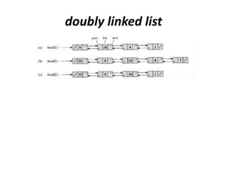
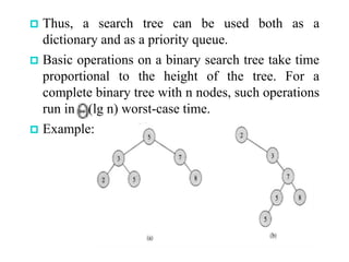
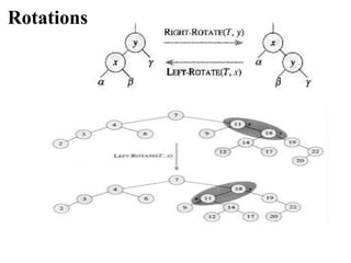
This chapter discusses various data structures including elementary data structures like stacks, queues, linked lists, binary trees, and hash tables. It then describes more complex data structures like red-black trees that balance binary search trees to guarantee logarithmic time operations. It also discusses augmenting data structures by adding size fields to support dynamic order statistics queries in logarithmic time.

1. Chapter 4
Data structures

2. Chapter about..
• Elementary data structures
• Hash tables
• Binary search trees
• Red black trees
• Augmenting data structures

3. Elementary data structures
• Stacks and queues
• Linked lists
• Implementing pointers and objects
• Binary trees
• Representing rooted trees
• The representation of dynamic sets by simple
data structures that use pointers.
• Complex data structures can be fashioned
using pointers.

4. Stacks and queues
• In a stack, the element deleted from the set is
the one most recently inserted: the stack
implements a last-in, first-out, or LIFO, policy.
• In a queue , the element deleted is always the
one that has been in the set for the longest
time: the queue implements a first-in, first-
out, or FIFO, policy.

5. Stacks
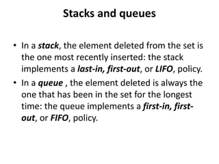
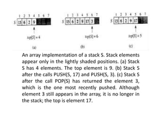
• INSERT operation on a stack  PUSH
• DELETE operation POP.
• top[S] that indexes the most recently inserted
element.
• The stack consists of elements S[1..top[S]], where
S[1] is the element at the bottom of the stack and
S[top[S]] is the element at the top.
• When top [S] = 0, the stack contains no elements
and is empty
• If an empty stack is popped, stack underflows,
which is normally an error.
• If top[S] exceeds n, the stack overflows.

6. An array implementation of a stack S. Stack elements
appear only in the lightly shaded positions. (a) Stack
S has 4 elements. The top element is 9. (b) Stack S
after the calls PUSH(S, 17) and PUSH(S, 3). (c) Stack S
after the call POP(S) has returned the element 3,
which is the one most recently pushed. Although
element 3 still appears in the array, it is no longer in
the stack; the top is element 17.

7. Queue
INSERT operation on a queue ENQUEUE,
DELETE operation DEQUEUE; like the stack
operation POP, DEQUEUE takes no element
argument.
The FIFO property of a queue causes it to
operate like a line of people in the registrar's
office. The queue has a head and a tail

9. Linked lists
• A linked list is a data structure in which the
objects are arranged in a linear order.
• Unlike an array, though, in which the linear
order is determined by the array indices, the
order in a linked list is determined by a pointer
in each object.
• Linked lists provide a simple, flexible
representation for dynamic sets

10. doubly linked list

11. Hash Table
• A hash table is an effective data structure for
implementing dictionaries. Although searching
for an element in a hash table can take as long
as searching for an element in a linked list.
• Direct-address tables

12. • Hash tables are a common approach to the
storing/searching problem.

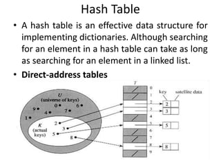
13. What is a Hash Table ?
 Each record has a special
field, called its key.
 In this example, the key is a
long integer field called
Number.
[ 0 ] [ 1 ] [ 2 ] [ 3 ] [ 4 ] [ 5 ]
. . .
[ 700]
[ 4 ]
Number 506643548
 Each record has a special
field, called its key.
 In this example, the key is a
long integer field called
Number.
 Each record has a special
field, called its key.
 In this example, the key is a
long integer field called
Number.

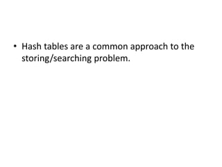
14. Collisions
 This is called a collision,
because there is already
another valid record at [2].
[ 0 ] [ 1 ] [ 2 ] [ 3 ] [ 4 ] [ 5 ] [ 700]
Number 506643548
Number 233667136
Number 281942902
Number 155778322
. . .
Number 580625685
Number 701466868
When a collision
occurs,
move forward until you
find an empty spot.

15. Hash functions
 uniform hashing
A good hash function satisfies (approximately) the
assumption of simple uniform hashing: each key is
equally likely to hash to any of the m slots.
 Hashing by division
 Hashing by multiplication
 Universal hashing.

16. Hashing by division
 division method for creating hash functions, we
map a key k into one of m slots by taking the
remainder of k divided by m. That is, the hash
function is
h(k) = k mod m

17. Hashing by multiplication
 The multiplication method for creating hash
functions operates in two steps. First, we multiply
the key k by a constant A in the range 0 < A < 1 and
extract the fractional part of kA. Then, we multiply
this value by m and take the floor of the result. In
short, the hash function is
 h(k) = m (k A mod 1)

18. Universal hashing
 choose the hash function randomly in a way that is
independent of the keys that are actually going to
be stored. This approach, called universal hashing
 h(x) = h(y) is precisely
 be a finite collection of hash functions that
map a given universe U of keys into the range
{0,1, . . . , m - 1}.

19. BINARY SEARCH TREES
 Search trees are data structures that support many
dynamic-set operations, including
 SEARCH,
 MINIMUM,
 MAXIMUM,
 PREDECESSOR,
 SUCCESSOR,
 INSERT, and DELETE.

20.  Thus, a search tree can be used both as a
dictionary and as a priority queue.
 Basic operations on a binary search tree take time
proportional to the height of the tree. For a
complete binary tree with n nodes, such operations
run in (lg n) worst-case time.
 Example:

21. Querying a binary search tree
 the SEARCH operation, binary search trees can
support such queries as MINIMUM, MAXIMUM,
SUCCESSOR, and PREDECESSOR.

22. RED-BLACK TREES
 the set operations are fast if the height of the
search tree is small; but if its height is large, their
performance may be no better than with a linked
list.
 Red-black trees are one of many search-tree
schemes that are "balance" in order to guarantee
that basic dynamic-set operations take O(lg n)
time in the worst case.

23. Properties of red-black trees
Each node of the tree now contains the fields color,
key, left, right, and p.
If a child or the parent of a node does not exist, the
corresponding pointer field of the node contains the
value NIL.
red-black properties:
1) Every node has a color either red or black.
2) Root of tree is always black.
3) There are no two adjacent red nodes (A red node
cannot have a red parent or red child).
4) Every path from root to a NULL node has same
number of black nodes

24. Example

25. Rotations

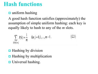
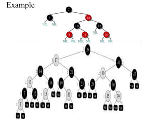
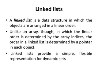
26. AUGMENTING DATA STRUCTURES
It introduced the notion of Dynamic order
statistics
size[x] = size[left[x]] + size[right[x]] + 1 .