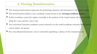
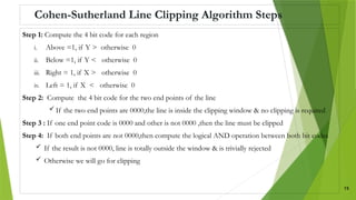
CHAPTER - FOUR
THE VIEWING PIPELINE
AND
PROJECTIONS
1
INTRODUCTION
 A viewing pipeline is just a sequence of transformations that every primitive has to undergo before it
is displayed.
 but the details of these transformations can vary slightly from package to package
 we refer to a different coordinate system after each transformation.
 For example, if we apply a translation we can think of this transformation as translating the origin of
the coordinate system to define a new (shifted) coordinate system.
 The same concept applies to rotations, scaling and other transformations.
2
2D Viewing Transformation Pipeline
3
1. The Modelling Transformation
 Modelling refers to the process of building our 3-D scene from a number of basic primitives
 All primitives start off in their own private coordinate system, and we call this the modelling coordinate
system.
 These primitives must be transformed to get them in the correct position, scale and orientation to
construct our scene.
 Once we have transformed all primitives to their correct positions we say that our scene is in world
coordinates
 In order to be able to render an image of a scene we need to define a virtual camera to take the picture.
4
2. Viewing Transformation
 The viewing transformation represents the positioning, direction and orientation of the virtual camera.
 This transformation defines a new coordinate system known as the viewing coordinate system.
 In this coordinate system the origin is normally at the position of the virtual camera, the camera ‘looks’
along the x-axis, and the y-axis is ‘up’.
 Any convenient Cartesian coordinate system referred to as the world coordinate reference frame can be
used to define the picture
 For a two-dimensional picture a view is selected by specifying a subarea of the total picture area
5
Cont’d …
6
The Viewing Pipeline
World Coordinates Viewport(Device) Coordinates
min
xw max
xw
min
yw
max
yw
Window
min
xv max
xv
min
yv
max
yv
Viewport
Cont’d …
 A world – coordinate area selected for display is called window. The object within the window area
displayed only.
 An area on a display device to which a window is mapped is called a viewport.
 The window defines what is to be viewed ,whereas the viewport defines where it is to be displayed . Both
are rectangular normally.
 Mapping of a part of a world coordinate scene to device coordinates is referred to as a viewing
transportation .
 The 2D dimensional viewing transformation is simply referred to as the window-to-viewport
transformation or the window transformation
7
Viewing Coordinate Reference Frame
 This coordinate system provides the reference frame for specifying the world coordinate window.
 We can set up the viewing coordinate system using the transformation between coordinate system.
 First, a viewing coordinate origin is selected at some point world position : ()
 To obtain the matrix for converting world-coordinate positions to viewing coordinates we do the
following
1) Translate the viewing origin to the world origin
2) Rotate to align the two coordinate reference frames
Mathematically, = R ∙ T
8
Window-to-Viewport Coordinate Transformation
9
 Consider a point () inside the clipping window and Let this point has to map to a position () inside
the viewport
Cont’d …
 Solving for () we have :
10
Clipping Algorithm
 Any procedure that identifies those portions of a picture that are either inside or outside of a specified
region of space is referred to as clipping algorithm or clipping
 The region against which an object is to be clipped is called a clip window
 Types of clipping
1) Point clipping
2) Line clipping
3) Area (polygon) clipping
4) Curve clipping
5) Text clipping
11
Point Clipping
12
Line Clipping
 Line clipping examines the end points of each line to see if they are in the window or not
 There is no need to clip lines with both end-points within the window
13
7
p
1
p
2
p
3
p
4
p
5
p
6
p
8
p
9
p
10
p
Before Clipping
1
p
2
p
5

p
6
p
7

p
8

p
After Clipping
Cohen-Sutherland Line Clipping Algorithm
 This is the efficient ,oldest and popular line clipping algorithm.
 Advantage: it is vastly reduced the number of line intersections that must be calculated.
 World space is divided into regions based on the window boundaries
 Each region has a unique four bit region code
 Region codes indicates the position of the regions with respect to the window
14
Top bit Bottom bit Right bit Left bit
Cohen-Sutherland Line Clipping Algorithm Steps
Step 1: Compute the 4 bit code for each region
i. Above =1, if Y > otherwise 0
ii. Below =1, if Y < otherwise 0
iii. Right = 1, if X > otherwise 0
iv. Left = 1, if X < otherwise 0
Step 2: Compute the 4 bit code for the two end points of the line
 If the two end points are 0000,the line is inside the clipping window & no clipping is required
Step 3 : If one end point code is 0000 and other is not 0000 ,then the line must be clipped
Step 4: If both end points are not 0000,then compute the logical AND operation between both bit codes
 If the result is not 0000, line is totally outside the window & is trivially rejected
 Otherwise we will go for clipping
15
Cont’d …
Step 5: Let the line has the end points () and ( )
 The y-coordinate of an intersection with a vertical window boundary can be calculated using:
 The x-coordinate of an intersection with a horizontal window boundary can be calculated using:
Step 6: After finding the intersection points compare with the point clipping algorithm
 Then choose which pair of intersection point satisfies the point clipping algorithm
 This pair of intersection point is visible inside the clipping window
16
Point:( , y) y = + m( - ) Left edge intersection
Point :( , y) y = + m( - ) Right edge intersection
Point:(x, ) x = + ( - ) /m Top edge intersection
Point :( , ) x = + ( - ) /m Bottom edge intersection , Where m=
Example
 Given a clipping window coordinates A(20,20) , B(60,20),C(60,40), D(20,40) using Cohen-Sutherland line
clipping algorithm , find the visible of the line joining the points P(40,80),Q(120,30)
Solution
point 4 bit code
P 1000
Q 0010
0000 (logical AND)
 As the bit code of the end points P,Q are not
0000 so clipping is needed
 Using logical AND P And Q the result is 0000
so we go for clipping.
Cont’d …
Find intersection points
Slope of the line , m = (30-80)/(120-40) = -5/8
1. Left-edge
y = + m( - ) => -5/8(20-40) +80 = 92.5 >
so,(,y) = (20 , 92.5), is rejected
2. Right – edge
y = + m( - ) => -5/8(60-40) +80 = 67.5 >
so,(,y) = (60 , 67.5), is rejected
3. Top – edge
x = + ( - )/m => 40 - 8/5(40-80) = 104 >
so,( x , ) = (104 , 40), is rejected
4. Bottom – edge
x = + ( - )/m => 40 – 8/5 (20 - 80) = 136 >
so,(x , ) = (136 , 20), is rejected
So, no intersection point satisfy the point clipping algorithm hence the line is not visible inside the clipping window 18
Exercise
1. Apply the Cohen-Sutherland line clipping algorithm to clip the line with (10,30) and (80,90) against the
window ABCD with A(20,20), B(90,20) , C(90,70) and D(20,70)
2. Apply the Cohen-Sutherland line clipping algorithm to clip the line with (20,30) and (70,80) against the
window ABCD with A(20,20), B(80,20) , C(90,60) and D(20,60)
19
PROJECTIONS
 It is the process of converting a 3D object into a 2D object.
 It is also defined as transformation of the object in projection plane or view plane.
 The transformation that handles all of this is known as the projection transformation.
20
Cont’d …
1. Parallel Projection : The projection lines of the two end-points are parallel:
 After they have passed through the image plane, and they continue to infinity without ever
meeting.
 Parallel projections have the property that objects that are further away from the virtual camera
do not appear smaller in the projected image.
 Parallel Projection use to display picture in its true shape and size.
 Parallel projections can be divided into two subtypes:
1. Orthographic (or orthogonal) projections
2. Oblique projections.
21
Cont’d …
 Basic difference between Orthographic(orthogonal) and Oblique projections are:
 In an orthographic projection the projection lines intersect with the image plane at right-angles
(they are orthogonal), whereas
 In an oblique projection they intersect at an angle (they are oblique).
 Both the projections are commonly used in engineering applications, particularly CAD software
22
Cont’d …
2. Perspective Projections: In this projection all projection lines converge to a point, the centre of
projection. In perspective projection farther away object from the viewer, small it appears.
 Here we can see that after passing through the image plane the projection lines of the two end
points intersect at a point.
 Perspective projections have the property that objects that are further away from the camera do
appear smaller.
23
Cont’d …
N.B
The human eye uses a perspective projection, as do all commercial cameras.
Parallel projections are a theoretical model of projection that can be useful in some computer
graphics applications.
 it is faster to compute, and so are used in some real-time applications such as computer
games.
24
The OpenGL Viewing Pipeline
 Now we will examine the viewing pipeline as it is defined by the OpenGL graphics package.
 OpenGL defines 3 matrices in its viewing pipeline:
1. model view matrix: this matrix combines the effects of the modelling and viewing transformations in
the general graphics pipeline.
2. The projection matrix: This represents the projection of 3-D viewing coordinate onto the image plane.
 OpenGL preserves the z-coordinate after projection and normalises the resulting coordinate system.
 Clipping is performed automatically based on the bounds we specify for the view volume
3. The viewport matrix: This matrix defines the part of the display that will be used for drawing
25
1. The Model view Matrix
 OpenGL maintains one matrix stack for each matrix in the viewing pipeline (i.e. there is one model view
matrix stack, one projection matrix stack and one viewport matrix stack).
 Therefore, before making any modifications to our current matrix (the top one on the stack) we must tell
OpenGL which matrix we are talking about.
 By this line of code we specifies to OpenGL that any subsequent transformations that we specify will
apply to the model view matrix:
 glMatrixMode(GL_MODELVIEW)
 Then we can use any of the following OpenGL functions to modify the current model view matrix:
26
 glTranslate
 glRotate
 glScale
 glLoadMatrix
 glMultMatrix
 gluLookAt
Cont’d …
 The first five functions we are used to define the modelling part of the modelview matrix.
 They are used to transform the primitives to form our 3-D scene in world coordinates.
 gluLookAt: This function is used to define the viewing part of the transformation
 recall that the viewing transformation defines the position, direction and orientation of a virtual camera.
 So the basic format of gluLookAt is: gluLookAt(x0, y0, z0, xref, yref, zref, Vx, Vy, Vz);
 The 1st
three arguments define a position (x0, y0, z0) in 3-D world coordinates. Simply this represents the
position of the virtual camera.
 The next three arguments define another position in 3-D world coordinates: (xref, yref, zref). This is the
position that the camera is ‘looking’ at.
 The last three arguments (Vx, Vy, Vz). These three values form a 3-D ‘up’ vector that defines the
orientation of the camera.
27
Cont’d …
 If the vector is perpendicular to the ‘look’ direction then it is projected so that it is perpendicular.
Example: the following 3 lines define a virtual camera positioned at (8, 0, 8) in world coordinates,
looking at the origin, and with the y-axis as ‘up’.
 NB: we have initialised the current modelview matrix to the identity matrix before defining the viewing
matrix.
 But, if the current matrix is not initialised the results will be undefined.
28
glMatrixMode(GL_MODELVIEW)
glLoadIdentity()
gluLookAt(8,0,8,0,0,0,0,1,0)
Cont’d …
 If you do not specify a viewing matrix in OpenGL the default parameters are:
(x0, y0, z0) = (0, 0, 0)
(xref, yref, zref) = (0, 0, -1)
(Vx, Vy, Vz) = (0, 1, 0)
 From the default parameters the camera is positioned at the origin, pointing along the negative z-axis,
with the y-axis as ‘up’.
 For example, the code example shown below displays two primitives (both 2-D rectangles) using the
same viewing transformation but different modelling transformations.
29
Cont’d …
# initialize modelview matrix to identity
glMatrixMode(GL_MODELVIEW)
glLoadIdentity()
# virtual camera is at (8, 0, 8) looking at the origin
# with the y-axis as ‘up’
gluLookAt(8,0,8,0,0,0,0,1,0)
glClear(GL_COLOR_BUFFER_BIT) # clear screen
# draw primitives
glPushMatrix() #remember viewing matrix
glRotatef(45,0,0,1) #rotate this primitive
glRecti(0,0,50,50) #draw rectangle
glPopMatrix() # restore viewing matrix
glPushMatrix() #remember viewing matrix
glTranslatef(200,0,0) # translate this primitive
glRecti(0,0,50,50) #draw rectangle
glPopMatrix() #restore viewing matrix
glFlush() # send all output to display
30
2. The Projection Matrix
 Depending on the type of projection required, OpenGL provides 4 alternative functions for specifying
the projection matrix:
1. gluOrtho2D
2. glOrtho
3. gluPerspective
4. glFrustum
1. gluOrtho2D:
 The gluOrtho2D function is intended for use with 2-D graphics only, and it does not allow you to
specify near and far clipping planes.
 The basic format of gluOrtho2D is: gluOrtho2D (xwmin, xwmax, ywmin, ywmax)
 The four arguments specify the x-coordinates of the left and right clipping planes, and the y-
coordinates of the bottom and top clipping planes 31
Cont’d …
 All coordinates are specified in the viewing coordinate system (i.e. the virtual camera is at the origin and
looking along the negative z-axis, and the y-axis is ‘up’).
 In 2-D graphics we just ignore the third coordinate (it is normally set to zero), so orthographic
projections are ideal and no near and far clipping planes are required.
 For example: look the below line code.
glMatrixMode(GL_PROJECTION)
glLoadIdentity()
gluOrtho2D(0.0, 640.0, 0.0, 480.0)
 From this line of code the 2-D orthographic projection will display all primitives with x-coordinate
between 0 and 640, and y-coordinate between 0 and 480.
32
Cont’d …
2. glOrtho
 It is similar to gluOrtho2D except that it allows us to specify near and far clipping planes, in addition
to the left, right, bottom and top ones.
 The basic format is: glOrtho (xwmin, xwmax, ywmin, ywmax, dnear, dfar)
 Here the six arguments represent the x-coordinates of the left and right clipping planes, the y-
coordinates of the bottom and top clipping planes, and the z-coordinates of the near and far clipping
planes.
For example:
glMatrixMode(GL_PROJECTION)
glLoadIdentity()
// arguments are left, right, bottom, top, near, far
glOrtho(-12, 12, -12, 12, 0, 30)
33
Cont’d …
3. gluPerspective
 If a perspective projection is required, OpenGL provides two alternative functions.
 The first is gluPerspective.
 The basic format is: gluPerspective (theta, aspect, dnear, dfar)
 NB: theta: represents the height angle of the perspective projection.
 The height angle is the angle between the top and bottom bounds of the image
 aspect: is the aspect ratio of the image (the ratio of the width to the height).
 dnear and dfar, are the z-coordinates of the near and far clipping planes.
 Example:- glMatrixMode(GL_PROJECTION)
glLoadIdentity()
gluPerspective(45, 1.0, 0.0, 50.0) 34
Cont’d …
4. glFrustum
 The OpenGL perspective projection routine allows you to specify the vertices of this frustum directly.
 The glFrustum basic format is: glFrustum (xwmin, xwmax, ywmin, ywmax, dnear, dfar)
 From glFrustum , the first 4 arguments are the x and y coordinates of the left, right, bottom and top
clipping planes at the near clipping plane.
 And the last two arguments, dnear and dfar, represent the z-coordinates of the near and far clipping planes.
 Therefore the positions of the four corners of the near clipping plane are (in viewing coordinates):
(xwmin, ywmin, dnear)
(xwmin, ywmax, dnear)
(xwmax, ywmin, dnear)
(xwmax, ywmax, dnear)
35
3. The Viewport Matrix
 The viewport matrix is defined slightly differently to the modelview and projection matrices.
 There is only one function for defining the viewport matrix
 The function is glViewport and its basic format is:
glViewport(xmin, ymin, xsize, ysize)
 (xmin, ymin) is the bottom-left corner of the viewport, in the coordinate system of the screen window
(whose origin is at the bottom-left).
 The arguments xsize and ysize are the size of the viewport in pixels.
 For example, assuming that we have a screen window of size 640x480, the following line defines the
viewport to be of size 300x300 and centred in the screen window.
glViewport(160, 90, 300, 300)
36
37
THANK YOU!
ANY QUESTIONS?

CHAPTER - 4 for software engineering (1).pptx

  • 1.
    CHAPTER - FOUR THEVIEWING PIPELINE AND PROJECTIONS 1
  • 2.
    INTRODUCTION  A viewingpipeline is just a sequence of transformations that every primitive has to undergo before it is displayed.  but the details of these transformations can vary slightly from package to package  we refer to a different coordinate system after each transformation.  For example, if we apply a translation we can think of this transformation as translating the origin of the coordinate system to define a new (shifted) coordinate system.  The same concept applies to rotations, scaling and other transformations. 2
  • 3.
  • 4.
    1. The ModellingTransformation  Modelling refers to the process of building our 3-D scene from a number of basic primitives  All primitives start off in their own private coordinate system, and we call this the modelling coordinate system.  These primitives must be transformed to get them in the correct position, scale and orientation to construct our scene.  Once we have transformed all primitives to their correct positions we say that our scene is in world coordinates  In order to be able to render an image of a scene we need to define a virtual camera to take the picture. 4
  • 5.
    2. Viewing Transformation The viewing transformation represents the positioning, direction and orientation of the virtual camera.  This transformation defines a new coordinate system known as the viewing coordinate system.  In this coordinate system the origin is normally at the position of the virtual camera, the camera ‘looks’ along the x-axis, and the y-axis is ‘up’.  Any convenient Cartesian coordinate system referred to as the world coordinate reference frame can be used to define the picture  For a two-dimensional picture a view is selected by specifying a subarea of the total picture area 5
  • 6.
    Cont’d … 6 The ViewingPipeline World Coordinates Viewport(Device) Coordinates min xw max xw min yw max yw Window min xv max xv min yv max yv Viewport
  • 7.
    Cont’d …  Aworld – coordinate area selected for display is called window. The object within the window area displayed only.  An area on a display device to which a window is mapped is called a viewport.  The window defines what is to be viewed ,whereas the viewport defines where it is to be displayed . Both are rectangular normally.  Mapping of a part of a world coordinate scene to device coordinates is referred to as a viewing transportation .  The 2D dimensional viewing transformation is simply referred to as the window-to-viewport transformation or the window transformation 7
  • 8.
    Viewing Coordinate ReferenceFrame  This coordinate system provides the reference frame for specifying the world coordinate window.  We can set up the viewing coordinate system using the transformation between coordinate system.  First, a viewing coordinate origin is selected at some point world position : ()  To obtain the matrix for converting world-coordinate positions to viewing coordinates we do the following 1) Translate the viewing origin to the world origin 2) Rotate to align the two coordinate reference frames Mathematically, = R ∙ T 8
  • 9.
    Window-to-Viewport Coordinate Transformation 9 Consider a point () inside the clipping window and Let this point has to map to a position () inside the viewport
  • 10.
    Cont’d …  Solvingfor () we have : 10
  • 11.
    Clipping Algorithm  Anyprocedure that identifies those portions of a picture that are either inside or outside of a specified region of space is referred to as clipping algorithm or clipping  The region against which an object is to be clipped is called a clip window  Types of clipping 1) Point clipping 2) Line clipping 3) Area (polygon) clipping 4) Curve clipping 5) Text clipping 11
  • 12.
  • 13.
    Line Clipping  Lineclipping examines the end points of each line to see if they are in the window or not  There is no need to clip lines with both end-points within the window 13 7 p 1 p 2 p 3 p 4 p 5 p 6 p 8 p 9 p 10 p Before Clipping 1 p 2 p 5  p 6 p 7  p 8  p After Clipping
  • 14.
    Cohen-Sutherland Line ClippingAlgorithm  This is the efficient ,oldest and popular line clipping algorithm.  Advantage: it is vastly reduced the number of line intersections that must be calculated.  World space is divided into regions based on the window boundaries  Each region has a unique four bit region code  Region codes indicates the position of the regions with respect to the window 14 Top bit Bottom bit Right bit Left bit
  • 15.
    Cohen-Sutherland Line ClippingAlgorithm Steps Step 1: Compute the 4 bit code for each region i. Above =1, if Y > otherwise 0 ii. Below =1, if Y < otherwise 0 iii. Right = 1, if X > otherwise 0 iv. Left = 1, if X < otherwise 0 Step 2: Compute the 4 bit code for the two end points of the line  If the two end points are 0000,the line is inside the clipping window & no clipping is required Step 3 : If one end point code is 0000 and other is not 0000 ,then the line must be clipped Step 4: If both end points are not 0000,then compute the logical AND operation between both bit codes  If the result is not 0000, line is totally outside the window & is trivially rejected  Otherwise we will go for clipping 15
  • 16.
    Cont’d … Step 5:Let the line has the end points () and ( )  The y-coordinate of an intersection with a vertical window boundary can be calculated using:  The x-coordinate of an intersection with a horizontal window boundary can be calculated using: Step 6: After finding the intersection points compare with the point clipping algorithm  Then choose which pair of intersection point satisfies the point clipping algorithm  This pair of intersection point is visible inside the clipping window 16 Point:( , y) y = + m( - ) Left edge intersection Point :( , y) y = + m( - ) Right edge intersection Point:(x, ) x = + ( - ) /m Top edge intersection Point :( , ) x = + ( - ) /m Bottom edge intersection , Where m=
  • 17.
    Example  Given aclipping window coordinates A(20,20) , B(60,20),C(60,40), D(20,40) using Cohen-Sutherland line clipping algorithm , find the visible of the line joining the points P(40,80),Q(120,30) Solution point 4 bit code P 1000 Q 0010 0000 (logical AND)  As the bit code of the end points P,Q are not 0000 so clipping is needed  Using logical AND P And Q the result is 0000 so we go for clipping.
  • 18.
    Cont’d … Find intersectionpoints Slope of the line , m = (30-80)/(120-40) = -5/8 1. Left-edge y = + m( - ) => -5/8(20-40) +80 = 92.5 > so,(,y) = (20 , 92.5), is rejected 2. Right – edge y = + m( - ) => -5/8(60-40) +80 = 67.5 > so,(,y) = (60 , 67.5), is rejected 3. Top – edge x = + ( - )/m => 40 - 8/5(40-80) = 104 > so,( x , ) = (104 , 40), is rejected 4. Bottom – edge x = + ( - )/m => 40 – 8/5 (20 - 80) = 136 > so,(x , ) = (136 , 20), is rejected So, no intersection point satisfy the point clipping algorithm hence the line is not visible inside the clipping window 18
  • 19.
    Exercise 1. Apply theCohen-Sutherland line clipping algorithm to clip the line with (10,30) and (80,90) against the window ABCD with A(20,20), B(90,20) , C(90,70) and D(20,70) 2. Apply the Cohen-Sutherland line clipping algorithm to clip the line with (20,30) and (70,80) against the window ABCD with A(20,20), B(80,20) , C(90,60) and D(20,60) 19
  • 20.
    PROJECTIONS  It isthe process of converting a 3D object into a 2D object.  It is also defined as transformation of the object in projection plane or view plane.  The transformation that handles all of this is known as the projection transformation. 20
  • 21.
    Cont’d … 1. ParallelProjection : The projection lines of the two end-points are parallel:  After they have passed through the image plane, and they continue to infinity without ever meeting.  Parallel projections have the property that objects that are further away from the virtual camera do not appear smaller in the projected image.  Parallel Projection use to display picture in its true shape and size.  Parallel projections can be divided into two subtypes: 1. Orthographic (or orthogonal) projections 2. Oblique projections. 21
  • 22.
    Cont’d …  Basicdifference between Orthographic(orthogonal) and Oblique projections are:  In an orthographic projection the projection lines intersect with the image plane at right-angles (they are orthogonal), whereas  In an oblique projection they intersect at an angle (they are oblique).  Both the projections are commonly used in engineering applications, particularly CAD software 22
  • 23.
    Cont’d … 2. PerspectiveProjections: In this projection all projection lines converge to a point, the centre of projection. In perspective projection farther away object from the viewer, small it appears.  Here we can see that after passing through the image plane the projection lines of the two end points intersect at a point.  Perspective projections have the property that objects that are further away from the camera do appear smaller. 23
  • 24.
    Cont’d … N.B The humaneye uses a perspective projection, as do all commercial cameras. Parallel projections are a theoretical model of projection that can be useful in some computer graphics applications.  it is faster to compute, and so are used in some real-time applications such as computer games. 24
  • 25.
    The OpenGL ViewingPipeline  Now we will examine the viewing pipeline as it is defined by the OpenGL graphics package.  OpenGL defines 3 matrices in its viewing pipeline: 1. model view matrix: this matrix combines the effects of the modelling and viewing transformations in the general graphics pipeline. 2. The projection matrix: This represents the projection of 3-D viewing coordinate onto the image plane.  OpenGL preserves the z-coordinate after projection and normalises the resulting coordinate system.  Clipping is performed automatically based on the bounds we specify for the view volume 3. The viewport matrix: This matrix defines the part of the display that will be used for drawing 25
  • 26.
    1. The Modelview Matrix  OpenGL maintains one matrix stack for each matrix in the viewing pipeline (i.e. there is one model view matrix stack, one projection matrix stack and one viewport matrix stack).  Therefore, before making any modifications to our current matrix (the top one on the stack) we must tell OpenGL which matrix we are talking about.  By this line of code we specifies to OpenGL that any subsequent transformations that we specify will apply to the model view matrix:  glMatrixMode(GL_MODELVIEW)  Then we can use any of the following OpenGL functions to modify the current model view matrix: 26  glTranslate  glRotate  glScale  glLoadMatrix  glMultMatrix  gluLookAt
  • 27.
    Cont’d …  Thefirst five functions we are used to define the modelling part of the modelview matrix.  They are used to transform the primitives to form our 3-D scene in world coordinates.  gluLookAt: This function is used to define the viewing part of the transformation  recall that the viewing transformation defines the position, direction and orientation of a virtual camera.  So the basic format of gluLookAt is: gluLookAt(x0, y0, z0, xref, yref, zref, Vx, Vy, Vz);  The 1st three arguments define a position (x0, y0, z0) in 3-D world coordinates. Simply this represents the position of the virtual camera.  The next three arguments define another position in 3-D world coordinates: (xref, yref, zref). This is the position that the camera is ‘looking’ at.  The last three arguments (Vx, Vy, Vz). These three values form a 3-D ‘up’ vector that defines the orientation of the camera. 27
  • 28.
    Cont’d …  Ifthe vector is perpendicular to the ‘look’ direction then it is projected so that it is perpendicular. Example: the following 3 lines define a virtual camera positioned at (8, 0, 8) in world coordinates, looking at the origin, and with the y-axis as ‘up’.  NB: we have initialised the current modelview matrix to the identity matrix before defining the viewing matrix.  But, if the current matrix is not initialised the results will be undefined. 28 glMatrixMode(GL_MODELVIEW) glLoadIdentity() gluLookAt(8,0,8,0,0,0,0,1,0)
  • 29.
    Cont’d …  Ifyou do not specify a viewing matrix in OpenGL the default parameters are: (x0, y0, z0) = (0, 0, 0) (xref, yref, zref) = (0, 0, -1) (Vx, Vy, Vz) = (0, 1, 0)  From the default parameters the camera is positioned at the origin, pointing along the negative z-axis, with the y-axis as ‘up’.  For example, the code example shown below displays two primitives (both 2-D rectangles) using the same viewing transformation but different modelling transformations. 29
  • 30.
    Cont’d … # initializemodelview matrix to identity glMatrixMode(GL_MODELVIEW) glLoadIdentity() # virtual camera is at (8, 0, 8) looking at the origin # with the y-axis as ‘up’ gluLookAt(8,0,8,0,0,0,0,1,0) glClear(GL_COLOR_BUFFER_BIT) # clear screen # draw primitives glPushMatrix() #remember viewing matrix glRotatef(45,0,0,1) #rotate this primitive glRecti(0,0,50,50) #draw rectangle glPopMatrix() # restore viewing matrix glPushMatrix() #remember viewing matrix glTranslatef(200,0,0) # translate this primitive glRecti(0,0,50,50) #draw rectangle glPopMatrix() #restore viewing matrix glFlush() # send all output to display 30
  • 31.
    2. The ProjectionMatrix  Depending on the type of projection required, OpenGL provides 4 alternative functions for specifying the projection matrix: 1. gluOrtho2D 2. glOrtho 3. gluPerspective 4. glFrustum 1. gluOrtho2D:  The gluOrtho2D function is intended for use with 2-D graphics only, and it does not allow you to specify near and far clipping planes.  The basic format of gluOrtho2D is: gluOrtho2D (xwmin, xwmax, ywmin, ywmax)  The four arguments specify the x-coordinates of the left and right clipping planes, and the y- coordinates of the bottom and top clipping planes 31
  • 32.
    Cont’d …  Allcoordinates are specified in the viewing coordinate system (i.e. the virtual camera is at the origin and looking along the negative z-axis, and the y-axis is ‘up’).  In 2-D graphics we just ignore the third coordinate (it is normally set to zero), so orthographic projections are ideal and no near and far clipping planes are required.  For example: look the below line code. glMatrixMode(GL_PROJECTION) glLoadIdentity() gluOrtho2D(0.0, 640.0, 0.0, 480.0)  From this line of code the 2-D orthographic projection will display all primitives with x-coordinate between 0 and 640, and y-coordinate between 0 and 480. 32
  • 33.
    Cont’d … 2. glOrtho It is similar to gluOrtho2D except that it allows us to specify near and far clipping planes, in addition to the left, right, bottom and top ones.  The basic format is: glOrtho (xwmin, xwmax, ywmin, ywmax, dnear, dfar)  Here the six arguments represent the x-coordinates of the left and right clipping planes, the y- coordinates of the bottom and top clipping planes, and the z-coordinates of the near and far clipping planes. For example: glMatrixMode(GL_PROJECTION) glLoadIdentity() // arguments are left, right, bottom, top, near, far glOrtho(-12, 12, -12, 12, 0, 30) 33
  • 34.
    Cont’d … 3. gluPerspective If a perspective projection is required, OpenGL provides two alternative functions.  The first is gluPerspective.  The basic format is: gluPerspective (theta, aspect, dnear, dfar)  NB: theta: represents the height angle of the perspective projection.  The height angle is the angle between the top and bottom bounds of the image  aspect: is the aspect ratio of the image (the ratio of the width to the height).  dnear and dfar, are the z-coordinates of the near and far clipping planes.  Example:- glMatrixMode(GL_PROJECTION) glLoadIdentity() gluPerspective(45, 1.0, 0.0, 50.0) 34
  • 35.
    Cont’d … 4. glFrustum The OpenGL perspective projection routine allows you to specify the vertices of this frustum directly.  The glFrustum basic format is: glFrustum (xwmin, xwmax, ywmin, ywmax, dnear, dfar)  From glFrustum , the first 4 arguments are the x and y coordinates of the left, right, bottom and top clipping planes at the near clipping plane.  And the last two arguments, dnear and dfar, represent the z-coordinates of the near and far clipping planes.  Therefore the positions of the four corners of the near clipping plane are (in viewing coordinates): (xwmin, ywmin, dnear) (xwmin, ywmax, dnear) (xwmax, ywmin, dnear) (xwmax, ywmax, dnear) 35
  • 36.
    3. The ViewportMatrix  The viewport matrix is defined slightly differently to the modelview and projection matrices.  There is only one function for defining the viewport matrix  The function is glViewport and its basic format is: glViewport(xmin, ymin, xsize, ysize)  (xmin, ymin) is the bottom-left corner of the viewport, in the coordinate system of the screen window (whose origin is at the bottom-left).  The arguments xsize and ysize are the size of the viewport in pixels.  For example, assuming that we have a screen window of size 640x480, the following line defines the viewport to be of size 300x300 and centred in the screen window. glViewport(160, 90, 300, 300) 36
  • 37.